Hypothesis Testing of Parameters for Ordinary Linear Circular Regression

ORDINARY LINEAR CIRCULAR REGRESSION

Abdul Ghapor Hussin

Centre for Foundation Studies in Science University of Malaya, 50603

KUALA LUMPUR

E-mail: [email protected]

Abstract

This paper presents the hypothesis testing of parameters for ordinary linear circular regression model assuming the circular random error distributed as von Misses distribution. The main interests are in testing of the intercept and slope parameter of the regression line. As an illustration, this hypothesis testing will be used in analyzing the wind and wave direction data recorded by two different techniques which are HF radar system and anchored wave buoy.

Key words: circular random variable, continuous linear variables, regression model, hypothesis testing, von Mises distribution.

1. Introduction

A circular random variable is a variable which takes values on the circumference of a circle, i.e. the angle is in the range (0, 2π ) radians or (00, 3600). This random variable must be analysed by techniques differing from those appropriate for the usual Euclidean type variables because the circumference is a bounded closed space, for which the concept of origin is arbitrary or undefined. A continuous linear variable is a random variable with realisations on the straight line which may be analysed by usual techniques.

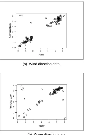
Ordinary linear circular regression model is applied when we wish to determine the relationship between a single circular explanatory variable X and a circular response variable Y. As an example is in the relationship of the measurements of wind and wave directions measured by an anchored buoy (Y) and radar (X) as shown in figures below, Sova (1995).

Figure below gives a simple (or even simplistic) scatter plot for each data set. In both cases the observations (direction, in radians) has been measured simultaneously by an anchored buoy (Y) and by radar (X). Although measurements are in radians, we will often use the more familiar degrees in informal discussion of the data. In this case we arbitrarily chose variate Y as the anchored buoy and variate X as radar.

6 5 4 3 2 1 0 6 5 4 3 2 1 0

Radar

A

n

c

h

o

red

bu

oy

regard those points at the top left and bottom right as outliers, but in relation to an ordinary linear circular regression model this is not so, because the measurements are on the circle or circumference, not a straight line. Since 1o is only 2o from 359o, the point (1o, 359o) on the simple scatter plot should not really be far from the ideal model y = x. In this respect, the simple scatter plot is misleading but it illustrate that an ordinary linear regression model which ignore the circularity of the data is equally misleading. Perhaps such scatter plots should be drawn on a torus which maintains the “wrapping” of the measurements scales. This shows the chief problem with ordinary linear regression when applied to circular variables and below we will propose an ordinary linear circular regressionmodel which is more suited to this form of data, Hussin (2004).

6 5 4 3 2 1 0 6 5 4 3 2 1 0

Radar

A

n

c

hor

ed buoy

(a) Wind direction data.

2. The Model and Parameters Estimation

Suppose for any circular observations (x y1, 1),...(xn,yn) of circular variables X

and Y, we propose a model of

yi = +α βxi +εi (mod2 )π (1)

where ε_i is a circular random error having a von Mises distribution with mean circular 0 and concentration parameter

κ

. An application when both X and Y are circular, for example in modelling a relationship for calibration between two instruments for wind direction, requires β ≈1.

Parameters α and β may be estimate by maximum likelihood estimation. Based on the von Mises density function, the log likelihood function for model (1) is given by

log ( , , ; ,..., , ,..., )

log( ) log ( ) cos( ).

L x x y y

n n I y x

n n i i α β κ π κ κ α β 1 1 0 2 = − − +

∑

− −

We differentiate log L with respect to α β , and κ to get α β , and κ which are given by

tan ,

tan ,

tan , ,

α π

π

=

⎛

⎝⎜ ⎞⎠⎟ > > ⎛

⎝⎜ ⎞⎠⎟+ < ⎛

⎝⎜ ⎞⎠⎟+ < > ⎧ ⎨ ⎪ ⎪ ⎪ ⎩ ⎪ ⎪ ⎪ − − − 1 1 1 0 0 0

2 0 0

S

C S C

S

C C

S

C S C

,

. (2)

sin( )

cos( )

β β α β α β 1 0 0 2 0 ≈ + − − − −

∑

∑

x y x

x y x

i i i

i i i

(3)

This expression for βˆ may be solved iteratively given some suitable “initial guesses” at the estimate. We can then update α and β and proceed iteratively. This iteration procedure will continue until the convergence criterion satisfied. Further the estimate of parameter concentration is given by

cos( )

κ = − ⎛_⎝⎜

∑

− −α β ⎞_⎠⎟

A

n yi xi

1 1

We can now proceed to obtain useful approximations using the results of Dobson (1978) who gives various simple approximations for the function A (ratio of the modified Bessel functions for the first kind of order one, and the first kind of order zero) for the von Mises concentration parameter,

κ

. For example, for

0 65. < <w 1, the approximation is

A w w w

w

− _≈ − +

−

1

2

9 8 3

8 1 ( )

( ) .

Thus by using maximum likelihood estimation, we have shown that α β, and κ

can be estimated iteratively. Since both the x and y are measurements of the same quantity, unity would be logical initial estimate of β, and so a possible initial estimate for iteration is β0 =1 0. in (2) and (3).

3. The Hypothesis Testing of Parameters

This section is concerned with testing hypotheses on α and β, i.e testing the hypothesis H₀:β =0(mod2π) vs H₁:β ≠0(mod2π) for the ordinary linear circular regression of the form

y_i = +α βx_i +ε_i (mod2π), i=1, ..., n,

using observations (x y1, 1), ..., (xn,yn) and assuming that εi are VM( , )0κ . It follows directly that the observations yi are VM(α β κ+ xi, ). In particular, our interest is in testing the hypotheses that H0:β =1 against H1:β ≠1 and

H0:α =0(mod2 ) against π H1:α ≠0(mod2π). In a practical application

α =0 and β =10. implies an exact relationship between the two variables.

For large κ , Mardia (1972), has shown that 2κS0 has a χ 2

distribution with n degrees of freedom where

{

}

S0 = n−

∑

cos(yi − −α βxi) .

Further, if S_{0 0,} and S_{0 1,} are the values of S₀ under H₀ and H₁ respectively, i.e. S_{0 1,} = S₀(α β,) and S_{0 0,} =S₀(α∗, )1 , say then for large κ ,

which gives 2 0 1 0 0 1 2

κ(S , −S , ) ~ χ . Further 2κS0 1, and 2κ(S0 1, −S0 0, ) may be

assumed to be independently distributed. Consequently, for testing H0 against

H1, the following F-statistic may be used

F1, n-2 =

(

)

( ) , ,

,

n S S

S

−2 0 1 − 0 0 0 1

.

In this section we will use the above result to test the hypothesesH₀:β =1 against H₁:β ≠1 and H₀:α =0(mod2π) against H₁:α ≠0

, ) 2

(mod π in order to make a comparison between the fitted model and the ideal model of y= x. Suppose that (α∗, )1 and (α β,) are the maximum likelihood estimates of the parameters under H₀:β =1 and H₁:β ≠1 respectively. Under

H₀:β =1, the log likelihood function is given by

logL nlog( ) nlogI ( ) cos(yi xi)

∗ _{= − − +}

∑

_{− −}

2π 0 κ κ α .

Differentiating logL∗ with respect to α gives,

∂

∂α κ α

log

sin( )

L

y_i x_i ∗

=

∑

− − .

Setting this equal to zero and simplifying we get

tan sin( )

cos( ) , α∗ ∗ ∗ = − − =

∑

∑

y x y x S C i i i i say. Hence α π π ∗ − ∗ ∗ ∗ ∗ − ∗ ∗ ∗ − ∗ ∗ ∗ ∗ = ⎛ ⎝ ⎜ ⎞ ⎠

⎟ > >

⎛ ⎝ ⎜ ⎞

⎠

⎟ + <

⎛ ⎝ ⎜ ⎞

⎠

⎟ + < > ⎧ ⎨ ⎪ ⎪ ⎪ ⎩ ⎪ ⎪ ⎪ tan , tan ,

tan , ,

1

1

1

0 0

0

2 0 0

S

C S C

S

C C

S

C S C

,

Therefore

(

)

and the test statistic is given by

F1, n-2 =

(

)

( ) _{, ,}

,

n S S

S

−2 _{0 1} − _{0 0}

0 1

.

The same technique can be used to test the hypothesis that H₀:α =0(mod2π)

against H₁:α ≠0(mod2π). Suppose that ( ,0 β∗) and ( , )α β are the maximum likelihood estimates of the parameters under H₀:α =0(mod2π) and

H₁:α ≠0(mod2π) respectively. Under H₀:α =0(mod2π), the log likelihood function is given by

logL nlog( ) nlogI ( ) cos(yi xi)

∗ _{= − − +}

∑

₋

2π 0 κ κ β .

Differentiating logL∗ with respect to β gives,

∂

∂β κ β

log

cos( )

L

xi yi xi

∗

=

∑

− .

This may be solved iteratively for β∗ and it can be shown that

β β β

β

∗ ∗

∗

∗

= + −

−

∑

∑

0

0

2

0

x y x

x y x

i i i

i i i

sin( )

cos( ),

where β₀∗ is an initial estimate of β∗. Hence

{

}

S_{0 0,} = n−

∑

cos(y_i −β∗x_i) , and S_{0 1,} =

{

n−

∑

cos(y_i − −α β x_i)

}

.

We will use the same F-statistic as above to test the hypothesis for intercept α.

4. Application and Conclusion

In this section we will apply the results of the hypothesis testing and will use the wind and wave direction data as our examples. Suppose variable X is the observation (directions) measured by radar and variable Y is the observation (directions) measured by anchored buoy. The scatter plots of the data set in Figure 1, indicate that there is generally a linear relationship between the directions taken by radar and anchored buoy with β ≈1. We assume that each

where ε represents departures from the straight line implicit in the model, also called circular random errors, and are distributed as a von Mises distribution with circular mean 0, and concentration parameter κ , i.e. ε ~VM( , )0κ .

Estimates for the wind direction data are given in Table 1, together with their approximate standard errors.

Parameter Estimate St. error

α 0.153 6.479x10-2

β 0.976 1.596x10-2

κ 7.337 0.882

Table 1: Parameter estimates for wind direction data.

Testing the null hypothesis that α is equal to0mod(2π), gave an F-statistic equal to 5.275 which we compare with F(1,127). The null hypothesis is rejected at the 5% significance level indicating a non-zero α is required. However, testing the null hypothesis that β equals 1, gives F=2.217, and we draw the conclusion that the null hypothesis can not be rejected at the 5% significance level.

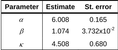
Table 2 give the estimates of wave direction data together with their approximate standard errors.

Parameter Estimate St. error

α 6.008 0.165

β 1.074 3.732x10-2

κ 4.508 0.680

Table 2: Parameter estimates for wave direction data.

References

1. Dobson, A. J. Applied Statistics, 27, (1978), pp. 345-347.

2. Mardia, K. V. Statistics of Directional Data. Academic Press, London, (1972).

3. Hussin, A.G., Fieller, N. R. J. and Eleanor, E. C. Journal of Applied Science & Technology, 8, Nos. 1 & 2 (2004), pp. 1 – 6.