The Cryosphere, 7, 1007–1015, 2013 www.the-cryosphere.net/7/1007/2013/ doi:10.5194/tc-7-1007-2013
© Author(s) 2013. CC Attribution 3.0 License.
EGU Journal Logos (RGB)
Advances in
Geosciences
Open Access
Natural Hazards
and Earth System
Sciences
Open Access
Annales
Geophysicae
Open Access
Nonlinear Processes
in Geophysics
Open Access
Atmospheric
Chemistry
and Physics
Open Access
Atmospheric
Chemistry
and Physics
Open Access
Discussions
Atmospheric
Measurement
Techniques
Open Access
Atmospheric
Measurement
Techniques
Open Access
Discussions
Biogeosciences
Open Access Open Access
Biogeosciences
DiscussionsClimate
of the Past
Open Access Open Access
Climate
of the Past
Discussions
Earth System
Dynamics
Open Access Open Access
Earth System
Dynamics
Discussions
Geoscientific
Instrumentation
Methods and
Data Systems
Open Access
Geoscientific
Instrumentation
Methods and
Data Systems
Open Access
Discussions
Geoscientific
Model Development
Open Access Open Access
Geoscientific
Model Development
DiscussionsHydrology and
Earth System
Sciences
Open Access
Hydrology and
Earth System
Sciences
Open Access
Discussions
Ocean Science
Open Access Open Access
Ocean Science
Discussions
Solid Earth
Open Access Open Access
Solid Earth
Discussions
The Cryosphere
Open Access Open Access
The Cryosphere
Discussions
Natural Hazards
and Earth System
Sciences
Open Access
Discussions
High sensitivity of tidewater outlet glacier dynamics to shape
E. M. Enderlin1,2, I. M. Howat1,2, and A. Vieli3
1Byrd Polar Research Center, The Ohio State University, 1090 Carmack Road, Columbus, Ohio 43210-1002, USA 2School of Earth Sciences, The Ohio State University, 275 Mendenhall Laboratory, 125 South Oval Mall, Columbus,
Ohio 43210-1308, USA
3Department of Geography, University of Zurich, Winterthurerstr. 190, 8057 Zurich, Switzerland Correspondence to: E. M. Enderlin ([email protected])
Received: 23 January 2013 – Published in The Cryosphere Discuss.: 19 February 2013 Revised: 22 May 2013 – Accepted: 23 May 2013 – Published: 28 June 2013
Abstract. Variability in tidewater outlet glacier behavior
un-der similar external forcing has been attributed to differences in outlet shape (i.e., bed elevation and width), but this de-pendence has not been investigated in detail. Here we use a numerical ice flow model to show that the dynamics of tide-water outlet glaciers under external forcing are highly sen-sitive to width and bed topography. Our sensitivity tests in-dicate that for glaciers with similar discharge, the trunks of wider glaciers and those grounded over deeper basal depres-sions tend to be closer to flotation, so that less dynamically induced thinning results in rapid, unstable retreat following a perturbation. The lag time between the onset of the pertur-bation and unstable retreat varies with outlet shape, which may help explain intra-regional variability in tidewater outlet glacier behavior. Further, because the perturbation response is dependent on the thickness relative to flotation, varying the bed topography within the range of observational uncertainty can result in either stable or unstable retreat due to the same perturbation. Thus, extreme care must be taken when inter-preting the future behavior of actual glacier systems using numerical ice flow models that are not accompanied by com-prehensive sensitivity analyses.
1 Introduction
While recent dynamic changes in marine-terminating outlet glaciers in Greenland and Antarctica are broadly correlated to climatic and oceanographic conditions, substantial spatio-temporal variability is evident (e.g., Howat et al., 2008; Moon and Joughin, 2008; McFadden et al., 2011; Moon et al., 2012; Walsh et al., 2012). Glaciers in close proximity,
and presumably exposed to similar environmental forcing, display contrasting behavior, suggesting that their dynamic response is largely dependent on individual characteristics, such as glacier shape (Meier and Post, 1987; Howat et al., 2007, 2008; Pfeffer, 2007).
thinning across a basal depression, as demonstrated by the rapid retreat of Helheim Glacier through a basal depression from 2004–2005 (Howat et al., 2007; Nick et al., 2009).
The timing and total magnitude of retreat will therefore de-pend on the basal topography and changes in glacier width, as rises in the bed and lateral constrictions in the surrounding bedrock walls should act as stabilizing points of ice conver-gence and higher friction (O’Neel et al., 2005; Jamieson et al., 2012). The response of a glacier to a perturbation at its front, therefore, should be highly dependent on the shape of the valley through which it flows (Pfeffer, 2007; Jamieson et al., 2012). Understanding this dependence is important for assessing regional variability in glacier behavior, identifying glaciers likely to exhibit large-scale changes in the near fu-ture, and constraining the impact of measurement uncertainty on model predictions of glacier behavior.
2 Model description
To test the influence of valley shape on tidewater glacier dynamics, we perform sensitivity tests using a moving-grid, depth-integrated, width-averaged numerical ice flow model (Vieli and Payne, 2005; Nick et al., 2009, 2010; Vieli and Nick, 2011) that includes lateral, basal, and along-flow stresses and uses an effective pressure-dependent sliding law and crevasse depth-dependent calving law (Benn et al., 2007; Nick et al., 2010). The depth integration of the model im-plicitly employs the Shallow Shelf Approximation, which is not fully appropriate for the entire model domain. How-ever, the model results obtained from the sensitivity tests examined herein should be valid along the regions of par-allel flow within the topographically confined trunks of fast-flowing tidewater outlet glaciers, as demonstrated by similar type model’s ability to reproduce changes in observed tide-water glacier behavior in numerous studies (see Nick et al., 2009, 2012; Vieli and Nick, 2011; Colgan et al., 2012). De-tails on the shape and surface mass balance parameteriza-tions, governing equaparameteriza-tions, boundary condiparameteriza-tions, and the ap-plied perturbation are provided below. The model discretiza-tion and implementadiscretiza-tion procedures are described in detail in Appendix A.
2.1 Shape and surface mass balance parameterizations
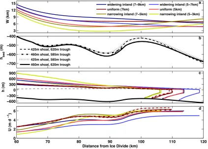
Each model glacier consists of a 120 km-wide inland ac-cumulation basin (ice sheet) that drains into a narrow, to-pographically confined outlet channel with a bed below sea level. Within the outlet, we assess the effects of both width and width gradient along-flow using six different width configurations that are within the range commonly ob-served for fast-flowing tidewater outlet glaciers in Green-land (Fig. 1a) and an idealized, over-deepened bed profile based on available bed elevation measurements (Fig. 1b). The cross-sectional shape of the outlet channel is also likely
to vary along-flow and could be incorporated into the model through the use of a shape factor, but its influence on ice flow is outside of the scope of the width-averaged sensitivity tests examined herein.
The bed elevation profiles are based on measurements for Helheim Glacier, Kangerdlugssuaq Glacier, and Jakob-shavn Isbræ in Greenland (CReSIS, http://www.cresis.ku. edu/data). We applied best-fit polynomials to along-flow bed elevation profiles from each glacier in order to extract eleva-tion and slope ranges, which were then used to construct an idealized bed (Fig. 1b, solid black line). A basal depression was included in the idealized bed profile because (1) similar depressions were found in all three bed elevation maps and (2) glaciers overlying basal depressions should be particu-larly sensitive to force balance perturbations, as described above. Using the uniform 7 km-width profile, we then as-sess the effects of bed elevation uncertainty using three ad-ditional bed profiles that fall within the≤50 m-uncertainty of current ice thickness observations (acquired from radio echo-sounding) (Bamber et al., 2013) as shown in Fig. 1b: shoal depth decreased by 35 m (dashed-dotted line), depres-sion depth decreased by 35 m (dashed line), and shoal and depression depths decreased by 35 m (dotted line).
The surface mass balance (SMB) rate is held constant in time and is prescribed as a function of distance from the equi-librium line. The magnitude of accumulation varies slightly for the different outlet shapes in order to maintain a similar interior ice thickness, as would be observed for glaciers fed by the same catchment area. The resulting SMB profiles fall within the typical range for Greenland outlet glaciers (Ettema et al., 2009; Burgess et al., 2010).
We include submarine melting along the base of the float-ing ice when present. Submarine meltfloat-ing is temporally con-stant but varies spatially as a function of distance from the grounding line (Rignot and Steffen, 2008), with the max-imum melt rate of 0.6 m d−1 occurring ∼1.2 km from the grounding line. Submarine melt rate magnitudes are based on the range of melt rates estimated for west Greenland out-let glaciers in Enderlin and Howat (2013).
2.2 Governing equations
Assuming no ice flow transverse to the glacier flowline, the temporal change in ice thickness can be determined using conservation of mass, such that
∂H ∂t = −
1
W
∂ (U W H )
∂x +B, (1)
3 6 9 12 15
W (km)
ï700 ï600 ï500 ï400
h bed
(m) 425m shoal, 620m trough 460m shoal, 585m trough 425m shoal, 585m trough 460m shoal, 620m trough
ï600 ï300 0 300 600 900
h (m)
widening inland (7ï9km) uniform (7km)
narrowing inland (7ï5km)
60 70 80 90 100 110 120
0 2 4 6
Distance from Ice Divide (km)
U (m d
ï
1 )
widening inland (5ï7km) uniform (5km)
narrowing inland (5ï3km) a
b
c
d
Fig. 1. Profiles of (a) width,W, and (b) bed elevation,hbed, along the outlet channel. Steady-state profiles of (c) surface elevation,h, and
(d) speed,U, obtained for each glacier shape. The different width and bed profiles used to obtain the steady-state profiles in (c) and (d) are distinguished by the line colors and styles specified in (a) and (b), respectively.
The governing force balance equation determined through conservation of momentum is
2 ∂
∂x
H v∂U ∂x
−β2U−H
W
5
U
2AW
1/3
=ρigH
∂h ∂x, (2)
whereβ2is the basal friction coefficient, Ais the rate fac-tor,ρi =917 kg m−3is the density of ice,gis gravitational acceleration,his the ice surface elevation, andvis the depth-averaged effective viscosity, which is defined as
v=A−1/3
∂U ∂x
−2/3
. (3)
The RHS of Eq. (2) is the gravitational driving stress, which is balanced by gradients in longitudinal stress (1st term LHS), basal resistance (2nd term LHS), and lateral resistance (3rd term LHS). The rate factor, A, is scaled with the cu-mulative strain rate (Ak∝
k P
j=1
∂U
∂x j) in order to account for strain heating along-flow. Using this scaling, the rate factor increases from a minimum of 3.5×10⁻²⁵ Pa−3s−1 at the divide to a maximum of 1.7×10⁻²⁴ Pa−3s−1 at the calv-ing front, correspondcalv-ing to a depth-averaged ice temperature range of−10◦C to−2◦C (Cuffey and Paterson, 2010).The
basal friction coefficient,β2, is parameterized as the product of the basal roughness factor and basal effective pressure. The same decreasing, piecewise linear function is used to parameterize the basal roughness factor for all simulations. We assume an open connection between the ocean and ice-bed interface, such that the water pressure increases with the bed depth and the basal effective pressure equals zero at the grounding line. The values selected forβ2are similar to those used to model Helheim Glacier (Nick et al., 2009), with values decreasing from a maximum ofβ2≈7.0×10¹⁰ Pa s m−1to zero as the ice approaches flotation.
The grounding line location is tracked using a flotation cri-terion, which has been successfully used in similar models to reproduce observed grounding line migration (e.g., Nick et al., 2009; Jamieson et al., 2012). The model employs a moving-grid that adjusts the grid spacing,1x, at each time step to precisely and continuously track the location of the grounding line by stretching/contracting the coordinate sys-tem to maintain1x∼=200 m (see Appendix A for details).
2.3 Boundary conditions
the point along the ungrounded portion of the glacier trunk where the surface crevasse depth equals the ice surface el-evation (Benn et al., 2007; Nick et al., 2010). The crevasse depth (dcrev)is calculated as follows:
dcrev=
Rxx
ρig
+ρw
ρi
dw, (4)
where ρw=1000 kg m−3 is the density of fresh water,
dw=10 m is the crevasse water height, and Rxx is the re-sistive stress, which is defined as follows:
Rxx=2
A−1∂U ∂x
1/3
. (5)
At the calving front, the gradients in longitudinal stress are in balance with the difference in hydrostatic pressure be-tween the ice and sea water such that
∂U ∂x =A
ρigH 4
1− ρi
ρsw
3
, (6)
whereρsw=1028 kg m−3is the density of sea water. 2.4 Model simulations
The simulated glaciers are initialized from the same speed and thickness profiles during a 200 yr spin-up period. The speed and thickness profiles obtained at the end of the spinup are used as the initial, steady-state profiles for the pertur-bation experiments. Here, we define steady-state based on inter-annual variability in the ice thickness at each grid cell: a simulated glacier is considered to have reached steady state if the ice thickness at each grid cell varies by<0.1 m yr−1. All simulations meet this criterion by the end of the 200 yr initialization period.
The transient simulations (i.e., perturbation experiments) are initialized using their respective steady-state speed and elevation profiles (Fig. 1c and d). A step reduction in resis-tive stress is applied at the calving front in order to simulate a reduction in backpressure resulting from ice tongue thinning and breakup, grounding line retreat, or m´elange weakening. This perturbation is applied at model time stepkby increas-ing horizontal stretchincreas-ing (i.e., decreasincreas-ing resistance to hori-zontal flow) at the front by a factor,S, equivalent to
Sk=1+
18 8k
, (7)
where8 is the difference in hydrostatic pressure between the ice and sea water. The stress perturbation,18, is the same for all simulations. By definingSin terms of the stress perturbation, we can express the perturbation in terms of an equivalent volume of ice tongue retreat (i.e., reduction in non-hydrostatic backstress). In our experiments, a con-stant value of18=1.00×10⁸Pa m is applied for the entire 30 yr-duration of the transient simulations. The magnitude of
the perturbation is equivalent to the loss of up to∼20 km3of floating ice from the terminus, which is of similar magnitude of the recent disintegration of Jakobshavn Isbræ’s floating ice tongue (Joughin et al., 2004).
3 Model results
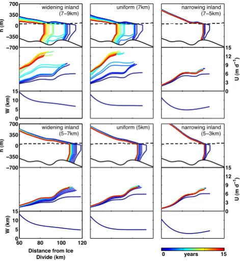
We focus our analysis of model results on the first 15 yr, following the application of the step perturbation when the magnitude of the simulated glacier response is largest (see Figs. 2–4). Application of the step perturbation results in instantaneous acceleration and retreat for all model runs (Figs. 2 and 3), reaching a maximum rate of thinning ranging from 11–17 m yr−1near the grounding line and decreasing to∼1 m yr−1∼35–55 km inland. Thinning and acceleration cause the discharge through the grounding line to peak within 6 months, increasing ∼5 % for the glaciers with narrower profiles and∼10 % for the two glaciers with the widest pro-files, then gradually stabilize (Fig. 4c). Following this ini-tial response, the evolution is bimodal: for the narrower and narrowing-inland glaciers, thinning and acceleration decline from their initial increase towards a new steady state with little overall retreat (Fig. 4a and b) and increase in ice dis-charge (Fig. 4c), whereas the two glaciers with the widest outlets reach flotation above the basal depression, triggering a much larger retreat and discharge increase.
The initial thickness profile determines the mode of re-sponse to the perturbation, as the initial steady-state thick-ness profiles of wider glaciers are closer to flotation above the basal depression and have a shallower surface slope in order to maintain the same discharge across the grounding line as narrower glaciers (Fig. 1c). Less initial thinning is therefore required to reach the threshold for unstable retreat, resulting in the ungrounding of a large section of the trunk. The delay in the onset of unstable retreat (i.e., lag time) is also controlled by the initial ice thickness above the basal depression, which varies by∼15 m here due to differences in convergence for glaciers that widen inland relative to those with parallel sides (Fig. 1c). Although the glacier that widens inland is initially thicker and therefore requires more time to thin to flotation (i.e., lag time), once unstable retreat is trig-gered, the total retreat and increase in discharge is of greater magnitude due to the feedback between retreat and increased cross-section of flow (Fig. 4).
ï700 ï350 0 350 700
h (m)
0 5 10 15
W (km)
0 3 6 9 12 15
U (m d
ï
1)
ï700 ï350 0 350 700
h (m)
60 80 100 120 0
5 10 15
W (km)
0 3 6 9 12 15
U (m d
ï
1) widening inland
(7ï9km)
uniform (7km) narrowing inland (7ï5km)
widening inland (5ï7km)
uniform (5km) narrowing inland (5ï3km)
Distance from Ice
Divide (km) 0 years 15
Fig. 2. Modeled annual elevation and speed profiles within the out-let channel (color coded for time, see colorbar) obtained using the 6 width configurations examined herein for 15 yr following the onset of the step perturbation. In the elevation profiles, the thin dashed gray line is the ice surface elevation required to remain grounded.
thickening within the depression, quadrupling the lag time between the perturbation and unstable retreat. Once unstable retreat is triggered, however, the increase in discharge and retreat of the grounding line into the basal depression is the same magnitude as for the glacier with the original, deeper shoal (Fig. 4). Thus, small differences in the thickness gradi-ent appear to have a similar, but stronger effect, as differences in the width gradient in controlling the timing of retreat.
4 Discussion and implications
All simulated glaciers that undergo unstable retreat into the depression show a significant lag time, of at least several years, between the perturbation and the onset of unstable re-treat, determined by the time needed to thin to flotation above the basal depression. This result is consistent with observa-tions from Columbia Glacier, Alaska, where a similar lag time between the onset of thinning and retreat following a period of glacier stability was observed in the 1980s (O’Neel et al., 2005). In southeast Greenland, however, a one- or two-year lag time between elevated ocean surface temperatures and the onset of rapid, unstable retreat has been observed (Howat et al., 2008). Differences in simulated and observed lag times are likely a consequence of starting the simulated glacier from an initial steady state, whereas glaciers in
south-ï700 ï350 0 350 700
h (m)
0 5 10 15
W (km)
0 3 6 9 12 15
U (m d
ï
1)
ï700 ï350 0 350 700
h (m)
60 80 100 120
0 5 10 15
W (km)
0 3 6 9 12 15
U (m d
ï
1)
460m shoal, 620m trough 425m shoal, 620m trough
460m shoal, 585m trough 425m shoal, 585m trough
Distance from Ice
Divide (km) 0 years 15
Fig. 3. Modeled annual elevation and speed profiles within the out-let channel (color coded for time, see colorbar) obtained using the 4 bed elevation profiles examined herein for 15 yr following the onset of the step perturbation. In the elevation profiles, the thin dashed gray line is the ice surface elevation required to remain grounded. As in Fig. 1, the different bed elevation profiles are distinguished by line style.
east Greenland may have been thinning since the mid 1990s (Krabill et al., 1999; Rignot et al., 2004). Simulated lag times are also likely to be influenced by the use of a simple flotation criterion to track grounding line migration rather than the more physically based contact problem described in Now-icki and Wingham (2007), although the flotation criterion has been successfully used in similar models to reproduce observed grounding line migration (e.g., Nick et al., 2009; Jamieson et al., 2012). Further, our model shows that small variations in width and basal topography can impart large differences in the timing of unstable retreat, which may ex-plain intra-regional variability found in Greenland. These ef-fects can be non-local, with inland variations in width and bed elevations influencing the stability of the grounding line on decadal timescales.
ï30 ï20 ï10 0
dx
front
(km)
widening inland (5ï7km) uniform (5km)
narrowing inland (5ï3km)
ï30 ï20 ï10 0
dx
gl
(km)
widening inland (7ï9km) uniform (7km)
narrowing inland (7ï5km)
0 1 2 3 4 5 6 7 8 9 10 11 12 13 14 15 0
0.1 0.2 0.3 0.4 0.5
Time (yrs)
dQ
gl
460m shoal, 620m trough 425m shoal, 620m trough 460m shoal, 585m trough 425m shoal, 585m trough
a
b
c
decreased depression depth
decreased shoal depth
Fig. 4. Time series of modeled (a) front position change, (b) grounding line position change, both relative to their respective initial positions, and (c) the fractional increase in grounding line discharge following the perturbation onset relative to the initial steady-state discharge.
of the interpolated bed elevation map available for Green-land (Bamber et al., 2013) may result in smoothing of the bed topography in coastal regions, potentially influencing the simulated response (Durand et al., 2011). Our results suggest that a similar problem may exist for width, as∼1 km of vari-ation in outlet width may cause stable or unstable response. Thus, simulations of topographically confined outlet glaciers with termini near flotation must be accompanied by comhensive sensitivity analyses to establish confidence in pre-dictions. Further, we suggest that similar sensitivity analyses should be completed using two- or three-dimensional models in order to assess the influence of glacier shape on grounding line stability for glaciers and ice streams with strong lateral convergence along their trunks.
5 Conclusions
Using a simple ice flow model applied to archetypal out-let shapes, we have confirmed that the dynamic response of glaciers under a given perturbation at the ice front is highly sensitive to along-flow variations in shape, shedding light on the high spatial and temporal variability observed in outlet glacier behavior. The response of a glacier overlying a basal depression is bimodal; a perturbation results in either a
grad-ual return to a new steady state with little thinning and retreat or triggers run-away, multi-kilometer retreat and tens to hun-dreds of meters of thinning. Whether or not a glacier will enter unstable retreat is dependent on its minimum thickness above flotation at the onset of the perturbation, which is in turn dependent on shape. For glaciers draining the same in-terior catchment, glaciers with wider steady-state grounding lines and those with deeper basal depressions will tend to be closer to flotation in the depression than narrower or shallow glaciers, and thus less dynamic thinning will be required to bring the ice within the depression to flotation.
and governed by the physics of ice flow. Thus, based on these sensitivity tests, we conclude that extreme care must be taken when analyzing numerical model results applied to actual glacier systems.
Appendix A
Model discretization and implementation procedures
The general discretization of the model is described in detail below. The complete Matlab®version of the model used in this paper can be obtained by contacting the corresponding author.
Several parameters must first be specified for use through-out the model, including ice density (ρi= 917 kg m−3), ocean water density (ρsw=1028 kg m−3), and gravita-tional acceleration (g=9.8 m s−2). The initial grid spac-ing (1x0) is used to construct the gridded length (x=
0 :1x0: length(x)) of the model domain. The choice of1x0
should be based on desired model resolution and computa-tion time, and was selected in this study as 200 m. At eachx, temporally fixed values for bed elevation and width (hbedand W, respectively) are prescribed. Estimates for the ice thick-ness (H) and surface velocity (U) must also be specified at each grid cell for model initialization.
Equation (2) is used to determine the new gridded veloci-ties for the model domain through iterative convergence. The partial differential and discretized forms of Eq. (2) are as fol-lows:
2 ∂
∂x
H v∂U ∂x
−β2U−H
W
5U 2AW
1/3
=ρigH
∂h ∂x
2
1x2 Hj+1/2vj+1/2Uj+1−Hj+1/2vj+1/2Uj (A1)
+Hj−1/2vj−1/2Uj−1−Hj−1/2vj−1/2Uj
−. . . ,
. . .+βj2U−Hj
Wj 5U
j
2AjWj 1/3
=ρigHj
hj+1−hj
1x
wherevis effective viscosity defined as follows:
vj=A−1j /3
Uj+1−Uj
1x
−2/3
(A2)
and subscripts are position indices. Equation (A1) describes the force balance between gradients in longitudinal stress (1st term LHS), basal drag (2nd term LHS), lateral drag (3rd term LHS), and gravitational driving stress (RHS). For proper con-vergence to occur, the longitudinal stress term must be cal-culated on the staggered grid, as indicated by the position indices in Eq. (A1). The lateral drag term must be linearized so that the equation can be written in matrix-vector form. The
linearization procedure is
−Hj
Wj 5U
j
2AjWj 1/3
= −Hj
Wj
5
2AjWj 1/3
Uj1/3=
−Hj
Wj
5
2AjWj 1/3
γjUj (A3)
whereγj=Uj−2/3for simplification.
The matrix-vector form of Eq. (A1) becomes
1 C2E2G2
C3E3 G3
. ..
Cc−1Ec−1Gc−1
−1 1
−1 1
. ..
−1 1
U1 U2 U3 .. . Uc−1
Uc
Uc+1
.. . Uterm = 0 T2 T3 .. . Tc−1
Tc
Tc+1
.. . Tterm , (A4) where
Cj =1x22 Hj−1/2vj−1/2
Ej= −1x22 Hj+1/2vj+1/2+Hj−1/2vj−1/2
−βj2−γjHWj
j
5 2AjWj
1/3
Gj=1x22 Hj+1/2vj+1/2
Tj=ρigHj hj+1−hj
1x :dcrevj < hj
Tj=Aj h
ρig
4 Hj
1− ρi
ρsw
i3
1x:dcrevj ≥hj
(A5)
and the subscriptcdenotes the calving front location and the subscript term denotes the end of the ice domain. The calv-ing front is located at the first ungrounded grid cell where surface crevasses generated by longitudinal stretching inter-sect sea level (Eqs. 4–6) and the end of the ice domain is located where the ice thickness reaches zero. The boundary conditions have already been incorporated in Eq. (A4) so that there is zero ice flux at the ice divide (U1=0) and the gradi-ents in longitudinal stress are in balance with the difference between the hydrostatic pressure of the ice and ocean water at the calving face, such that
Uj−1−Uj
1x =Aj
ρ ig 4 Hj
1− ρi
ρsw
3
. (A6)
The calving front boundary condition is applied from calv-ing face to the end of the ice domain in order to avoid the force imbalance that occurs for1h/1x= ∞. Ice-free grid cells are not included in the matrix-vector notation because their driving stress and velocity terms are equal to zero.
grid cell. This process is repeated iteratively until the differ-ence between the velocities calculated in consecutive itera-tions meets a prescribed tolerance.
The gridded velocities are used to determine the change in ice thickness using conservation of mass (Eq. 1), such that:
∂H ∂t = −
1
W ∂(UWH)
∂x
1Hj,t = −W1
j
h(UWH)
j+1,t−(UWH)j,t
1x
i
1t, (A7)
where the subscript t denotes the time and 1t= 0.001 yr=31 536 s is the time step. Using the results from Eq. (A7) and surface mass balance (including submarine melting),B, the new ice thickness at each grid cell is solved using:
Hj,t+1=Hj,t+1Hj,t+Bj,t1t. (A8) For a fixed-grid numerical model, the gridded velocities obtained for timetcan be used with the ice thickness values for timet+1 (Eq. A8) to determine the coefficient matrix for timet+1. Moving-grid numerical models must account for
the change in the grounding line position between timetand timet+1 in order to accurately model grounding line mi-gration (Pattyn et al., 2012). For the moving grid, the interp1 function in Matlab®can be used to interpolate ice thickness values between grid cells, allowing grid adjustment to the precise location where H meets the flotation criterion. To maintain an adjusted grid spacing similar to a target value,
1x0, the new grid spacing,1xt+1, can be calculated as
fol-lows:
1xt+1=
xgz,t+1
round xgz,t+1/1x0
, (A9)
where xgz,t+1 is the location of the grounding line and
“round” specifies that the divisor is rounded to the nearest integer value. The interp1 function is then used to interpo-late all variables that vary spatially (e.g., H, h, U, A, etc.) to the new grid spacing. The use of relatively small grid spac-ing ensures that no numerical diffusion is introduced into the model during this interpolation. Further, the continuous moving-grid grounding line tracking described in Eq. (A9) is in-line with the boundary theory of Schoof (2007) and can be used to accurately capture transient grounding line migration (Pattyn et al., 2012). The interpolated variables are then used as input for Eqs. (A1–A8) to solve for gridded ice thickness and velocity at timet+2.
Acknowledgements. We would like to thank Andy Aschwanden
and a second, anonymous reviewer for their useful comments. We would also like to thank Frank Pattyn for his insightful editorial comments. This work was funded by a NASA Earth and Space Science Fellowship to E. M. E.
Edited by: F. Pattyn
References
Amundson, J. M., Fahnestock, M., Truffer, M., Brown, J., L¨uthi, M. P., and Motyka, R. J.: Ice m´elange dynamics and implications for terminus stability, Jakobshavn Isbræ, Greenland, J. Geophys. Res., 115, F01005, doi:10.1029/2009JF001405, 2010.
Bamber, J. L., Griggs, J. A., Hurkmans, R. T. W. L., Dowdeswell, J. A., Gogineni, S. P., Howat, I., Mouginot, J., Paden, J., Palmer, S., Rignot, E., and Steinhage, D.: A new bed elevation dataset for Greenland, The Cryosphere, 7, 499–510, doi:10.5194/tc-7-499-2013, 2013.
Benn, D. I., Warren, C. R., and Mottram, R. H.: Calving processes and the dynamics of calving glaciers, Earth Sci. Rev., 82, 143– 179, doi:10.1016/j.earscirev.2007.02.002, 2007.
Burgess, E. W., Forster, R. R., Box, J. E., Mosley-Thompson, E., Bromwich, D. H., Bales, R. C., and Smith, L. C.: A spatially calibrated model of annual accumulation rate on the Green-land Ice Sheet (1958–2007), J. Geophys. Res., 115, F02004, doi:10.1029/2009JF001293, 2010.
Christoffersen, P., Mugford, R. I., Heywood, K. J., Joughin, I., Dowdeswell, J. A., Syvitski, J. P. M., Luckman, A., and Ben-ham, T. J.: Warming of waters in an East Greenland fjord prior to glacier retreat: mechanisms and connection to large-scale atmo-spheric conditions, The Cryosphere, 5, 701–714, doi:10.5194/tc-5-701-2011, 2011.
Colgan, W., Pfeffer, W. T., Rajaram, H., Abdalati, W., and Balog, J.: Monte Carlo ice flow modeling projects a new stable config-uration for Columbia Glacier, Alaska, c. 2020, The Cryosphere, 6, 1395–1409, doi:10.5194/tc-6-1395-2012, 2012.
Cuffey, K. M. and Paterson, W. S. B.: The physics of glaciers: Fourth edition, Elsevier, Amsterdam, 72–77, 2010.
Durand, G., Gagliardini, O., Favierm, L., Zwinger, T., and le Meur, E.: Impact of bedrock description on model-ing ice sheet dynamics, Geophys. Res. Lett., 38, L20501, doi:10.1029/2011GL048892, 2011.
Enderlin, E. M. and Howat, I. M.: Submarine melt rate estimates for floating termini of Greenland outlet glaciers (2000–2010), J. Glaciol., 59, 213, doi:10.3189/2013JoG12J049, 2013.
Ettema, J., van den Broeke, M. R., van Meijgaard, E., van de Berg, W. J., Bamber, J. L., Box, J. E., and Bales, R. C.: Higher sur-face mass balance of the Greenland ice sheet revealed by high-resolution climate modeling, Geophys. Res. Lett., 36, L12501, doi:10.1029/2009GL038110, 2009.
Gudmundsson, G. H., Krug, J., Durand, G., Favier, L., and Gagliar-dini, O.: The stability of grounding lines on retrograde slopes, The Cryosphere, 6, 1497–1505, doi:10.5194/tc-6-1497-2012, 2012.
Holland, D. M., Thomas, R. H., de Young, B., Mibergaard, M. H., and Lyberth, B.: Acceleration of Jakobshavn Isbræ triggered by warm subsurface ocean waters, Nature Geosci., 1, 659–664, doi:10.1038/ngeo316, 2008.
Howat, I. M., Joughin, I., and Scambos, T. A.: Rapid changes in ice discharge from Greenland outlet glaciers, Science, 315, 1559– 156, doi:10.1126/science.1138478, 2007.
Howat, I. M., Joughin, I., Fahnestock, M., Smith, B. E., and Scam-bos, T. A.: Synchronous retreat and acceleration of southeast Greenland outlet glaciers 2000–2006: ice dynamics and coupling to climate, J. Glaciol., 54, 646–660, 2008.
outlet glaciers in Greenland, J. Glaciol., 56, 601–613, 2010. Jamieson, S. S. R., Vieli, A., Livingstone, S. J., Cofaigh, C. ´O.,
Stokes, C., Hillenbrand, C. D., and Dowdeswell, J. A. : Ice-stream stability on a reverse bed slope, Nature Geosci., 5, 799– 802, doi:10.1038/ngeo1600, 2012.
Joughin, I. and Alley, R. B.: Stability of the West Antarctic ice sheet in a warming world, Nature Geosci., 4, 506–513, doi:10.1038/ngeo1194, 2011.
Joughin, I., Abdalati, W., and Fahnestock, M.: Large fluctuations in speed on Greenland’s Jakobshavn Isbræ glacier, Nature, 432, 608–610, 2004.
Krabill, W., Frederick, E., Manizade, S., Martin, C., Sonntag, J., Swift, R., Thomas, R., Wright, W., and Yungel, J.: Rapid thinning of parts of the southern Greenland Ice Sheet, Science, 283, 1522– 1524, doi:10.1126/science.283.5407.1522, 1999.
McFadden, E. M., Howat, I. M., Joughin, I., Smith, B. E., and Ahn, Y.: Changes in the dynamics of marine terminating outlet glaciers in west Greenland (2000-2009), J. Geophys. Res., 116, F02022, doi:10.1029/2010JF001757, 2011.
Meier, M. F. and Post, A.: Fast tidewater glaciers, J. Geophys. Res., 92, 9051–9058, 1987.
Moon, T. and Joughin, I.: Changes in ice front position on Green-land’s outlet glaciers from 1992 to 2007, J. Geophys. Res., 113, F02022, doi:10.1029/2007JF000927, 2008.
Moon, T., Joughin, I., Smith, B., and Howat, I.: 21st-century evo-lution of Greenland outlet glacier velocities, Science, 336, 576– 578, doi:10.1126/science.1219985, 2012.
Motyka, R. M., Truffer, M., Fahnestock, M., Mortensen, J., Rysgaard, S., and Howat, I.: Submarine melting of the 1985 Jakobshavn Isbræ floating tongue and the trigger-ing of the current retreat, J. Geophys. Res., 116, F01007, doi:10.1029/2009JF001632, 2011.
Nick, F. M., Vieli, A., Howat, I. M., and Joughin, I.: Large-scale changes in Greenland outlet glacier dynamics triggered at the ter-minus, Nature Geosci., 2, 110–114, doi:10.1038/ngeo394, 2009. Nick, F. M., van der Veen, C. J., Vieli, A., and Benn, D. I.: A phys-ically based calving model applied to marine outlet glaciers and implications for the glacier dynamics, J. Glaciol., 56, 781–794, 2010.
Nick F. M., Luckman A., Vieli, A., van der Veen, C. J., van, As D., van de Waal, R. S. W., Pattyn, F., Hubbard, A. L., and Floricioiu, D.: The response of Petermann Glacier, Greenland, to large calv-ing events, and its future stability in the context of atmospheric and oceanic warming, J. Glaciol., 58, 229–239, 2012.
Nowicki, S. M. J. and Wingham, D. J.: Conditions for a steady ice sheet-ice shelf junction, Earth Planet. Sci. Lett., 265, 246–255, doi:10.1016/j.epsl.2007.10.018, 2008.
O’Neel, S., Pfeffer, W. T., Krimmel R., and Meier, M.: Evolving force balance at Columbia Glacier, Alaska, dur-ing its rapid retreat, J. Geophys. Res., 110, F03012, doi:10.1029/2005JF000292, 2005.
Pattyn F., Schoof, C., Perichon, L., Hindmarsh, R. C. A., Bueler, E., de Fleurian, B., Durand, G., Gagliardini, O., Gladstone, R., Goldberg, D., Gudmundsson, G. H., Huybrechts, P., Lee, V., Nick, F. M., Payne, A. J., Pollard, D., Rybak, O., Saito, F., and Vieli, A.: Results of the Marine Ice Sheet Model Intercomparison Project, MISMIP, The Cryosphere, 6, 573–588, doi:10.5194/tc-6-573-2012, 2012.
Pfeffer, W. T.: A simple mechanism for irreversible tide-water glacier retreat, J. Geophys. Res., 112, F03S25, doi:10.1029/2006JF000590, 2007.
Rignot, E. and Steffen, K.: Channelized bottom melting and sta-bility of floating ice shelves, Geophys. Res. Lett., 35, L02503, doi:10.1029/2007GL031765, 2008.
Rignot, E., Braaten, D., Gogineni, S. P., Krabill, W. B., and McConnell, J. R.: Rapid ice discharge from south-east Greenland glaciers, Geophys. Res. Lett., 31, L10401, doi:10.1029/2004GL019474, 2004.
Schoof, C.: Ice sheet grounding line dynamics: Steady-states, stability, and hysteresis, J. Geophys. Res., 112, F03S28, doi:10.1029/2006JF000664, 2007.
Vieli, A. and Nick ,F. M.: Understanding and modelling rapid dy-namic changes of tidewater outlet glaciers: Issues and implica-tions, Surv. Geophys., 32, 437–458, 2011.
Vieli, A. and Payne, A. J.: Assessing the ability of numerical ice sheet models to simulate grounding line migration, J. Geophys. Res., 110, F01003, doi:10.1029/2004JF000202, 2005.