R E S E A R C H
Open Access
A biplot correlation range for group-wise
metabolite selection in mass spectrometry
Youngja H Park
1, Taewoon Kong
2*, James R. Roede
3, Dean P. Jones
4,5and Kichun Lee
6** Correspondence:
[email protected];twkong@
gatech.edu 6
Department of Industrial Engineering, Hanyang University, Seoul 04763, South Korea
2Industrial and Systems Engineering,
Georgia Institute of Technology, Atlanta, GA 30332, USA Full list of author information is available at the end of the article
Abstract
Background:Analytic methods are available to acquire extensive metabolic
information in a cost-effective manner for personalized medicine, yet disease risk and diagnosis mostly rely upon individual biomarkers based on statistical principles of false discovery rate and correlation. Due to functional redundancies and multiple layers of regulation in complex biologic systems, individual biomarkers, while useful, are inherently limited in disease characterization. Data reduction and discriminant analysis tools such as principal component analysis (PCA), partial least squares (PLS), or orthogonal PLS (O-PLS) provide approaches to separate the metabolic
phenotypes, but do not offer a statistical basis for selection of group-wise metabolites as contributors to metabolic phenotypes.
Methods:We present a dimensionality-reduction based approach termed‘biplot correlation range (BCR)’that uses biplot correlation analysis with direct orthogonal signal correction and PLS to provide the group-wise selection of metabolic markers contributing to metabolic phenotypes.
Results:Using a simulated multiple-layer system that often arises in complex biologic systems, we show the feasibility and superiority of the proposed approach in comparison of existing approaches based on false discovery rate and correlation. To demonstrate the proposed method in a real-life dataset, we used LC-MS based metabolomics to determine spectrum of metabolites present in liver mitochondria from wild-type (WT) mice and thioredoxin-2 transgenic (TG) mice. We select discriminatory variables in terms of increased score in the direction of class identity using BCR. The results show that BCR provides means to identify metabolites contributing to class separation in a manner that a statistical method by false discovery rate or statistical total correlation spectroscopy can hardly find in complex data analysis for predictive health and personalized medicine.
Keywords:Feature selection, Biplot correlation, Metabolomics
Introduction
Contemporary analytic methods, such as liquid chromatography-mass spectrometry (LC-MS) [1, 2], gas chromatography-mass spectrometry (GC-MS) [3, 4], and proton nuclear magnetic resonance (1H NMR) spectroscopy [5, 6], provide information-rich data sets that can be of substantial value in biomedical research and, in principle, can be developed with bioinformatics procedures for routine healthcare [7–9]. Challenges in clinical use exist at two levels, reliable extraction of metabolic features from spectro-scopic data and reliable identification of metabolic features associated with health
characteristics. Substantial progress has been made in data extraction, with several high-quality routines available. For instance, recent introduction of adaptive processing by apLCMS [10] provides a systematic approach to reduce noise and extract relative quantification of > 7000 metabolic features in 50 aliquots of human plasma in 20 min (2); current improvements in data processing have demonstrated that > 12,000 meta-bolic features can be extracted [11]. This high volume of information, which is inher-ently multivariate, presents challenges to reliable use in health prediction and disease management.
Statistical methods based upon the principles of false discovery rate (FDR) are avail-able to correct for large numbers of comparisons in multiple hypothesis testing of metabolomics data [12]. These methods are useful to identify potential biomarkers as-sociated with disease or disease risk while controlling the expected proportion of incor-rectly rejected null hypotheses (type-I error). This approach is effective because it yields single biomarker candidates that can be rigorously tested and directly used in health research and clinical practice.
Individual biomarkers, however, can be of limited value in practical use. For instance, biomarkers with a relatively good specificity (e.g., 0.9) and sensitivity (e.g., 0.9) still re-sult in large numbers of misclassifications, i.e., one diagnosis in ten will be wrong and one in ten will be missed. While several factors can contribute, a central limitation is that statistical procedures examining individual variables do not consider how variables interact and combine. In complex pathobiology, individuals with the same genetic mu-tation have different disease phenotypes, e.g., some patients with a sickle cell disease mutation have hemolytic crises while others with the same mutation have painful crises with bony infarcts, acute chest syndrome or only mild anemia [13]. At the molecular level, functional redundancies and multiple interacting levels of regulation within net-work structures result in second-order and higher order interactions that allow the same pathway to respond differently among individuals. Additionally, metabolic re-sponses can be conditional because of genetic and epigenetic differences, as well as dif-ferences in diet, environment or health behaviors. For instance, decreased plasma cystine in response to zinc supplementation may not only be due to zinc-dependent ef-fects on cystine uptake and conversion to glutathione by tissues [14,15], but also upon intestinal absorption, renal loss, rates of transcription of relevant regulatory systems and past exposures that alter epigenetic regulation [16, 17]. Such complexity means that individual biomarkers can rarely, if ever, be universally useful. Consequently, statis-tical approaches equivalent to FDR, when conducting multiple comparisons, are needed to identify metabolites important in group-wise (e.g., metabolic pathway and network) behavior, thereby providing rigorous bases to include metabolic interactions within complex metabolic datasets for improved disease classification and health prediction.
discriminatory patterns is derived from established data reduction and multivariate techniques, (i.e., PCA, PLS, and OPLS), and methods to discover new variables describ-ing otherwise hidden, lower-dimensional structure. Extracted representations are trans-formed into new data (score vectors) using a relatively small number of newly selected variables (loading vectors comprised of the original variable contributions). These new variables have improved power to discriminate samples linked to phenotype, such as pathological characteristic (Y as response variable). A specific advantage of this ap-proach is that multiple components, none of which may be significantly associated with Y when evaluated individually by statistical tests such as FDR, can interact to discrim-inate Y using BCR.
In development of the proposed approach, we relied upon a commonly used graph-ical technique of matching score plots and loading plots, called as a biplot method [18]. Cloarec et al. used a two-step approach to facilitate biomarker detection in 1H NMR spectroscopy by graphically coupling a loading vector from OPLS and the correlation of each variable with response Y [19]. In the development of BCR, we similarly create a loading vector for each metabolite contributing to separation. A subsequent selection of metabolites with defined correlation interval (e.g., 95%) is used to determine metabo-lites related with defined classes. This allows individual metabometabo-lites contributing to sep-aration to be visualized in respective loading plots, thereby providing a rigorously defined approach to identify metabolites contributing to group behavior. We explore whether BCR would determine a correlation range using scores and loadings in PCA, extending them to PLS and OPLS, and biomarkers for the purpose of discrimination analysis of mass spectral data from mitochondria isolated from wild-type (WT) mice and thioredoxin-2 (Trx2) TG mice. This study showed that BCR provides means to se-lect metabolites contributing to class separation in a manner that can complement FDR in complex data analysis for predictive health and personalized medicine.
Methods
In this section, we introduce the theoretical background of a biplot and its interpret-ation from a correlinterpret-ation viewpoint with regard to the development of biplot correlinterpret-ation statistics.
Biplot
A biplot is constructed by using a dimensionality-reduction technique to obtain a low-dimensional approximation to a transformed version of a data matrix, X in size n×p, where n and p denote the number of samples (observations) and features (vari-ables), respectively. The most popular dimensionality-reduction technique is singular value decomposition (SVD) which brings forth principal component analysis (PCA). Other techniques such as multidimensional scaling and partial least squares (PLS, also called projection to latent structures) are also available [20–22]. They, however, share the same spirit with SVD in a sense that the low-dimensional approximation ofXoften unravels hidden structures in X by maintaining inter-sample distances as much and capturing as much variation ofXas possible.
We find loading vectorsajof sizep× 1, j = 1,…,p, and their associated score vectorstj of size n× 1. Using SVD, we exactly obtain loading vector aj by an eigenvector of the sample covariance matrix and score vectortjby
tj¼Xaj¼ aTjx1⋯aTjxn
h iT
:
Score vector tj corresponding to loading vector aj represents new coordinates of n data on the axis of aj. Themth component [aj]m describes the amount of contribution of the original (before-transformation)mth variable to the construction of new axisaj.
Simply speaking, a larger [aj]mvalue is associated with more weight for themth vari-able in new axisaj. In practical use, before the application of dimensionality reduction, one could apply unit variance scaling for each column in X to provide all variables an equal weight. This scaling step, optional, depends on the domain characteristic of the data. For example, many biologic processes are determined by high abundance compo-nents, and because of this, variance scaling can sometimes result in loss of useful infor-mation by decreasing the contribution of more relevant, high-abundance variables and increasing contribution of non-relevant, low abundance variables.
We order loading vectors, a1,…,ap,according to their associated eigenvalues andp score vectors,t1,…, tpwill follow accordingly. Then we rewrite the data matrix X asX
¼Pp
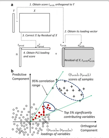
j¼1tjaTj: A biplot is formed by the first two dominant terms from two scatterplots of ([t1]i, [t2]i) for i = 1, …, n, and ([a1]m, [a2]m), denoted by !am, for m = 1, …, pthat share a common set of axes. In essence, excluding the constant term, the sample co-variance matrix approximates to XTX≅a1tT1t1aT1þ⋯þaktTktkaTk.Fig.1 (a) shows an ex-emplary biplot that has the simplified combination of a principal component score plot by‘+’markers and a principal component loading plot by‘o’markers.
Biplot correlation range
We present an interpretation of the direction and magnitude in a biplot in terms of correlation among variables and relate it to a procedure for biplot based discrimination analysis. Using the approximation of the sample covariance matrix in the construction of a biplot, the sample covariance between the qth and rth variables, dcovðxq;xrÞ, is given by
dcov xq;xr
¼XTX
q;r≅a1t T 1t1aT1
q;rþ a2t T 2t2aT2
q;r
¼½ a1qtT1t1½ a1rþ½ a2qtT2t2½ a2r¼ !aq;!ar
where 〈∙,∙〉represents an inner product with a weight vector ½tT
1t1tT2t2:It implies that the inner product between !aqand !ar corresponds to a covariance measure between the two variables. Observe that !aq and !ar are shown as two loading vectors in a
biplot. Then, given loading vector !aq¼ð½a1q;½a2qÞ, it is straightforward that the
direc-tion of!arshould be the same as that of!aq to maximize
a1
½ qt
T
1t1½ a1rþ½ a2qt T
2t2½ a2r¼‖!aq‖ ‖!ar‖cosθ≤‖!aq‖ ‖!ar‖;
d
corr xq;xr
¼ dcov xq;xr
ffiffiffiffiffiffiffiffiffiffiffiffiffiffiffiffiffiffiffiffiffiffiffiffiffiffiffiffiffiffiffiffiffiffiffiffiffiffiffiffiffiffiffiffiffiffiffiffiffiffi dcov xq;xq
dcov xð r;xrÞ
q ≅ a
! q;!ar
ffiffiffiffiffiffiffiffiffiffiffiffiffiffiffiffiffiffiffiffiffiffiffiffiffiffiffiffiffiffiffiffiffiffiffiffiffiffiffiffi
a !
q;!aq
a !
r;!ar
q ¼ cosθ:
Overall, the direction of !aj for thejth variable linking to correlation of variables is the direction to which the variable contributes in increasing scores on new axesa1and a2. Similarly, the magnitude of !a j is associated with the variable’s contribution in
a
b
Fig. 1aThe combination of a principal component score plot and a principal component loading plot,
called a biplot, is used to illustrate the concept of biplot correlation range. Based on the“+”score plot
values and the associated ellipse (broken line), a 95% confidence interval is calculated for projection onto the corresponding loading plot (small circles). Filled red circles contribute to scores within the 95% correlation
range, while the thick-lined ellipse represents the top 5% of features contributing to the“+”class.bThe flow of
magnitude of the score increasing, linking to covariance of variables. For the sake of convenience,!ajis used as the contributing direction of thejth variable.
When dimensionality-reduction techniques such as PLS and OPLS other than SVD approximate data matrix X in a similar fashion, the BCR approach is applied similarly using their loading vectors. Among numerous dimensionality-reduction techniques im-plemented and tested, we choose the combination of direct signal correction and PLS to obtain components able to separate response vectorYwith interpretability [23]. The flow of the decomposition is shown in Fig. 1(b). We extract a signal score vector,t(
or-tho), orthogonal to response vectorY with maximum variance in data matrixX. In spe-cific, for Y^, the projection ofY on the column space ofX, we numerically obtain the eigenvector with the largest eigenvalue, set to bet(ortho), in a subspace ofX orthogonal
to Y^ , ðI−Yð^ Y^TYÞ^ −1Y^TÞX;and then compute its loading vector aðorthoÞ¼XTtðorthoÞ ðtT
ðorthoÞtðorthoÞÞ −1
. We consider tðorthoÞaTðorthoÞ as a residual inX in the task of explaining
Y. Then we perform PLS with input data asX−tðorthoÞaTðorthoÞ, corrected by theY
-orthog-onal signal in X, and output dataY, obtaining its first score vector, t(pred), and loading vector, a(pred). We note that the use of direct signal correction inXby the first orthog-onal component beforehand helps the first component of PLS to effectively capture Y-separating patterns in X and produces interpretability when using the two compo-nents. Finally, we approximate data matrix X into one orthogonal component and an-other predictive component as follows:
X≅tðpredÞaTðpredÞþtðorthoÞaTðorthoÞ:
Score and loading vectors in the above decomposition retain the same interpretation as in PCA. We notice that the decomposition without an orthogonal component is equivalent to PLS and that numerous orthogonal and PLS components are possible in addition to various feature scaling methods. Typically, some kind of cross validation in combination with the domain characteristic of features is used to optimize the separ-ability of the whole procedure.
correlation range is invariant to the scaling of score vectors in consideration of the di-agonal lines from the zero. Finally, the top 5% (τ) of variables in magnitude of contrib-uting direction!ajare selected. Note that the stringency can be increased by use of top 1% or 0.5% of such variables. These features, illustrated as filled circles in the solid el-lipsoid, greatly contribute to the group label in a covariance (magnitude) sense. We perform the above procedures with scores of each group label, generating selected fea-tures per group label, as in Figs. 3(a)and5(a), and finally obtaining the union of them. Since the selected features are treated equally as long as they are within the top 5% cri-terion, post-analysis such as ordering them by correlation, covariance,p-values, or vari-able importance projection (VIP) values will be possible [24]. By default, we filter out variables of which individual regression performance measures with response Y are weak. Practically, we test if the p-value of a logistic regression model with responseY and the raw values of each individual variable xiis greater than 0.10, without control-ling familywise error rate or false discovery rate, to deem features of weak separability. Depending on the nature of variables and the problem domain, one could adopt other performance measures and tests such as Pearson correlation, Spearman’s rank correl-ation, p values of linear regression, and classification accuracy of logistic regression. This step eliminates unnecessary noisy features that act as contributing features in a collective sense from the previous step. We repeat the above steps for each group label, and the outcomes of these steps are lists of greatly contributing features for each group label.
This BCR approach is based on the graphical use of a biplot in that scores and load-ings are used collectively. BCR, however, enables discrimination analysis and a feature selection procedure using the interpretation of loading vectors while the biplot ap-proach provides only a graphical presentation of scores and loadings. We note that BCR relies upon the approximation of data matrix X≅t1aT1þt2aT2 using orthogonal and predictive components and the statistical properties of loading vector !a j and score vector !t j and it provides a structured approach to select features collectively significant.
Results
To test the BCR approach, we performed a simulation study and compared it with some existing methods. Then, we applied it to a real-life example.
Simulation and comparisons
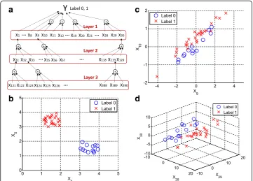
We first generated a data matrix X (200 × 1000) and a response vector Y (200 × 1), comprising 200 samples and 1000 variables. Each element ofYwas a Bernoulli random variable with a success probability of 0.4, so 16 elements ofYwere set to 1 on average, while the remaining 24 elements were set to 0. To generate 1000 variables, we used a three-layer network structure shown in Fig.2.
In the first layer, the first 30 variables were generated to have high separation in Y: forp= 1,…, 4,
xpU 0ð ;1Þ þ0:8−2Y;
xpU 0ð ;1Þ−1:2−2Y;
where U(a, b) is a random variable from a uniform distribution of range a and b. It means variables from x1to x4individually had a high positive correlation withY label 0, whereas variables x5to x8highly correlated withYlabel 1. In specific, the correlation between each of variables from x1to x4andYwas 0.9576 ± 0.0075 (average ± standard deviation) throughout the simulation, and that between each of variables x5to x8andY was 0.9577 ± 0.0075. Figure2(b) shows plots of realizations of x1and x5and the afore-mentioned pattern that clearly and individually separateY. The first eight variables in the first layer represent strong individual variables that should be used to identify pathological conditions. Forp= 9, 12,…, 18,
xpxpþ1
T
N 0þY 0 0½ :5T;A
;
and forp= 19, 22, 25, 28,
xpxpþ1xpþ2
TN 0þ
Y 1 2 3½ T;B
;
where A¼ 1 0:4 0:4 0:4
; B¼
12 10 8 10 12 10
8 10 12
2 4
3
5;and N(μ,∑) represents a multivariate
nor-mal distribution with mean μand covariance∑. Figure2(c) shows plots of realizations
a
b
c
d
Fig. 2aA data model was created for 200 samples, each with 1000 measured variables. The model has three layers of interaction of variables x that contribute to the response Y. Layer 1 contains 30 variables,
including eight strong variables (x1to x8) and other group-wise variables (x9to x30). Each of the variables in
Layer 1 is determined by three variables in Layer 2, and each in Layer 2 by three variables in Layer 3. The
remaining 610 variables are randomly assigned.bTwo strong variables, x1and x5, individually separate the
two labels of response Y.cTwo strong variables, x9and x10, jointly separate the two labels of response Y.
of x9and x10that collectively separateY. Figure2(d) also illustrates that realizations of x28, x29and x30, generated as above, clearly and jointly discriminateY.The variables xi, i = 9,…, 30, in the first layer represent strong group-wise variables that clearly discrim-inate pathological conditions. The next 90 variables from x31to x120in the second layer and the next 270 variables from x121to x390 in the third layer were generated so that the variables contribute to the overall responseYin a composite and aggregate manner. For instance, x1in the first layer is clearly separable by the combination of x31, x32and x33, in the second layer. In specific, the generation of the three variables is based on the value of x1so that the sum of the three will be close to x1as follows: given x1, we inde-pendently generate u1, u2and u3from U(0,1) andϵfrom, Nð0;x101Þ. Then, we set
x31¼ u1
u1þu2þu3 ðx1þϵÞ;
x32¼ u2
u1þu2þu3 ðx1þϵÞ;
x33¼ u3
u1þu2þu3 ðx1þϵÞ;
which brings x31+x32+x33=x1+ϵ. The correlation between the sum of the three and x1 was 0.9730 ± 0.0085 throughout the simulation, and the generation method was similarly applied to the according matches in Fig. 2 (a). The remaining 610 variables from x391to x1000, comprising a noise layer, were randomly and independently gener-ated from N(0, 1) to avoid a strong correlation withY in order to simulate inherent noise. To better simulate the effect of randomness in noise, the p-value of a linear-regression fitting of Y with each xi from the 610 variables was controlled so that p-value≥δi, whereδiwas set to 0, 0.03, 0.05, or 0.10. The condition,δi=0, represents that the variables are completely random noise and some of them can be significant, and the condition, δi=0.10, represents the generated variables are deemed insignificant by significance level 0.10. The simulated three-layer structure is an example of multiple layers of metabolic interactions and regulation in complex biological systems. For in-stance, a biological system for nutritional metabolomics reflects such a layered struc-ture with linked transports [25]. To further simulate biological systems with fewer biomarkers, we also used the two-layer structure of layers 1 and 2 only, in which the remaining 880 variables were simulated noise, and the one-layer structure of only layer 1, in which the remaining 930 variables were simulated noise. To compare them with random-noise systems as a baseline performance, we also used a structure, denoted by noise layer structure, in which the total 1000 variables are simulated noise. The vari-ables as simulated noise were generated as described above by varyingδi.
Hochberg [12] and the other one (FDR2), by Benjamini and Yekutieli, considers mul-tiple testing under dependency [28]. We also mention that another version of FDR using p-values from logistic regression was tested but that no variables are found throughout the experiments. Thus, we dropped logistic regression based FDR in the following results. We chose STOCSYO as a representative method using correlation measures and FDR as using p-values. The BCR approach used the first orthogonal and the first predictive components from OPLS. The selection of important variables in
a
b
Fig. 3This figure illustrates feature selection using BCS for a simulated data set from the model in Fig.2.aA biplot for the first orthogonal and predictive components is shown, clearing separating the two labels of
response Y with a 95% correlation range for each label.bThe corresponding loading plot, a zoomed-in version
of the dotted-line rectangle in (a), is shown; the top 5% significantly contributing variables found from Layer 1,
2, and 3 are shown as red squares, blue diamonds, and black triangles, respectively. The eight strong variables
(x1to x8) in the plot are clearly distinguishable and positioned accordingly to the labels. For example, the
STOCSYO was set as the cut-off value of a correlation coefficient corresponding to significance levels varying from 1 to 20% [19, 26, 29]. The top percentile (τ) in BCR and the q-value for FDR also varied from 1 to 20%. We note that the adopted levels for the methods are not strictly comparable metrics by themselves, yet we compare them in that they are used in practice to adjust the number of se-lected variables.
Figure3 (a) and (b) show the scores and loadings, respectively, for the BCR method using a multiple-layer data set: in the loading plot, red squares, blue diamonds, and black triangles represent variables that are deemed to be greatly contributing from layers 1, 2, and 3, respectively. We note that the first eight variables (x1to x8) were cor-rectly found, and several additional variables from layers 2 and 3 were also detected. We notice that the loadings of the eight strong variables (x1to x8) are greatly larger than those of others, for examples, layer 2 variables (x9to x30) in the predictive compo-nent axis corresponding to loading vector a(pred) as shown in Fig. 3 (b). It is under-standable in view of that the loading vector in PLS is obtained as slope coefficients to predict X corrected by the Y-orthogonal signal, X−tðorthoÞaT
ðorthoÞ, by the score vector. We notice that the PLS score vector is calculated on the direction which maximizes the covariance between X and Y. It is worth mentioning that the first eight variables were positioned accordingly to the labels. The position of x1, for example, was aligned to the direction of label 0, in accordance with the behavior of x1in Fig.2(b). This im-plies that an increase in x1results in an increase in label 0.
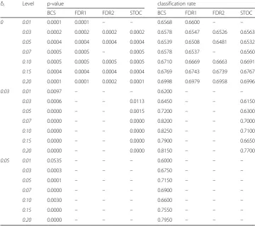
performance increases as the number of the detected noise variable increases. It indi-cates that the detected noise variables are discriminative in the classification task. The p-values and classification accuracy for the two-layer, the one-layer, and the noise-layer structures in Additional files1,2and3: Tables S3–S5, respectively, show the similar re-sult as in Table5for the detected noise variables.
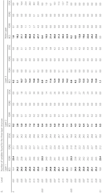
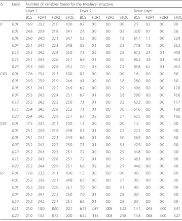
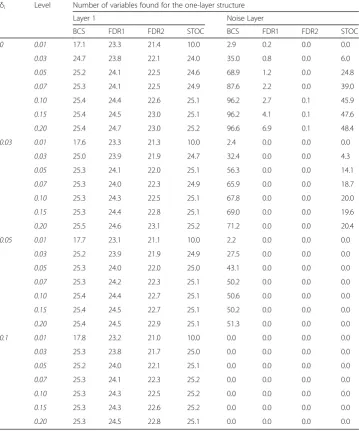
The averaged numbers found by the various methods in the two-layer structure are presented in Table 5; For all levels, BCR still found more variables in layer 1 than STOCSYO and FDR. The BCR method also found more variables in layer 2 than STOCSYO and FDR. We also observe STOCSYO also detected more variables in layer 2 than FDR. The averaged numbers found by the various methods in the one-layer structure are presented in Table1; BCR outperformed STOCSYO and FDR for all levels with regard to the number of variables found. The average number of variables in each layer filtered out by the BCS method in the layer structures along with the averaged
Table 2Average numbers of variables found in the simulation study for the two-layer structure
δi Level Number of variables found for the two-layer structure
Layer 1 Layer 2 Noise Layer
BCS FDR1 FDR2 STOC BCS FDR1 FDR2 STOC BCS FDR1 FDR2 STOC
0 0.01 16.9 23.2 21.0 10.0 0.2 0.0 0.0 0.0 2.9 0.2 0.0 0.0
0.03 24.8 23.9 21.8 24.1 2.4 0.0 0.0 0.3 32.0 0.7 0.0 5.6
0.05 25.0 24.0 22.1 24.7 5.3 0.0 0.0 1.8 61.7 1.1 0.0 22.9
0.07 25.1 24.1 22.3 24.8 5.8 0.1 0.0 2.3 77.8 1.8 0.0 35.2
0.10 25.2 24.2 22.4 25.0 7.1 0.2 0.0 2.8 87.2 2.4 0.1 44.0
0.15 25.1 24.3 22.6 25.1 6.9 0.1 0.0 3.0 86.2 3.8 0.1 44.3
0.20 25.3 24.6 22.8 25.2 7.0 0.3 0.0 2.9 85.8 6.2 0.1 44.2
0.03 0.01 17.6 23.4 21.3 10.0 0.7 0.0 0.0 0.0 1.6 0.0 0.0 0.0
0.03 24.9 23.9 21.9 24.6 4.1 0.0 0.0 1.8 28.0 0.0 0.0 3.0
0.05 25.1 24.1 22.2 24.9 6.2 0.0 0.0 2.9 49.6 0.0 0.0 12.0
0.07 25.3 24.3 22.4 25.1 6.7 0.1 0.0 2.8 59.0 0.0 0.0 16.0
0.10 25.3 24.2 22.5 25.0 7.1 0.1 0.0 3.2 62.2 0.0 0.0 17.7
0.15 25.4 24.5 22.8 25.2 7.1 0.1 0.0 3.0 61.6 0.0 0.0 18.0
0.20 25.4 24.5 22.9 25.1 6.7 0.2 0.0 2.7 62.5 0.0 0.0 18.6
0.05 0.01 17.5 23.1 21.1 10.0 1.1 0.0 0.0 0.0 1.2 0.0 0.0 0.0
0.03 25.1 23.9 21.9 24.8 5.3 0.1 0.0 2.2 22.2 0.0 0.0 0.0
0.05 25.1 24.1 22.3 24.9 6.6 0.1 0.0 3.0 36.9 0.0 0.0 0.0
0.07 25.2 24.1 22.2 25.0 7.1 0.1 0.0 3.1 42.9 0.0 0.0 0.0
0.10 25.2 24.3 22.5 25.1 7.2 0.0 0.0 2.9 44.8 0.0 0.0 0.0
0.15 25.2 24.3 22.6 25.1 7.2 0.1 0.0 2.9 46.3 0.0 0.0 0.0
0.20 25.2 24.4 22.9 25.1 6.8 0.2 0.0 2.9 44.6 0.0 0.0 0.0
0.1 0.01 17.8 23.3 21.1 10.0 1.5 0.0 0.0 0.0 0.0 0.0 0.0 0.0
0.03 25.2 23.8 22.1 24.8 6.5 0.0 0.0 2.7 0.0 0.0 0.0 0.0
0.05 25.2 23.9 22.0 25.1 7.0 0.0 0.0 3.1 0.0 0.0 0.0 0.0
0.07 25.2 24.1 22.2 25.0 7.0 0.1 0.0 2.8 0.0 0.0 0.0 0.0
0.10 25.2 24.2 22.7 25.1 6.6 0.1 0.0 2.8 0.0 0.0 0.0 0.0
0.15 21.0 13.0 8.60 20.1 6.75 .087 .005 3.22 14.1 .043 .000 5.41
p-values are presented in Additional files 4 and 5: Tables S6 and S7 according to the noise condition and tested level. Clearly, the number of the filtered variables increases as the noise conditions and levels increase. For example, the number of the filtered var-iables for levels ≤0.05 is quite much less than those for levels >0.05.It also increases as the structure moves from the three layers to the noise layers, which means increasing randomness. Consistently, most of the filtered variables appeared in the last noise layer, which practically demonstrates the use of the filtering step. For example, in the two-layer structure with noise condition 0 and level 0.10, the average number of the fil-tered variables in the noise layer is 64.69 while that in layer 1 is 0.52 and that in layer 2 is 10.18. Though small in number, the filtered variables in layer 1 partly explains the BCR never finds all 30 variables in layer 1.
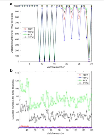
Additionally, Fig.4and figures in Additional file6: Figure S1 show the number of the selected variables by the four tested methods during the 1000 iterations in noise
Table 3Average numbers of variables found in the simulation study for the one-layer structure
δi Level Number of variables found for the one-layer structure
Layer 1 Noise Layer
BCS FDR1 FDR2 STOC BCS FDR1 FDR2 STOC
0 0.01 17.1 23.3 21.4 10.0 2.9 0.2 0.0 0.0
0.03 24.7 23.8 22.1 24.0 35.0 0.8 0.0 6.0
0.05 25.2 24.1 22.5 24.6 68.9 1.2 0.0 24.8
0.07 25.3 24.1 22.5 24.9 87.6 2.2 0.0 39.0
0.10 25.4 24.4 22.6 25.1 96.2 2.7 0.1 45.9
0.15 25.4 24.5 23.0 25.1 96.2 4.1 0.1 47.6
0.20 25.4 24.7 23.0 25.2 96.6 6.9 0.1 48.4
0.03 0.01 17.6 23.3 21.3 10.0 2.4 0.0 0.0 0.0
0.03 25.0 23.9 21.9 24.7 32.4 0.0 0.0 4.3
0.05 25.3 24.1 22.0 25.1 56.3 0.0 0.0 14.1
0.07 25.3 24.0 22.3 24.9 65.9 0.0 0.0 18.7
0.10 25.3 24.3 22.5 25.1 67.8 0.0 0.0 20.0
0.15 25.3 24.4 22.8 25.1 69.0 0.0 0.0 19.6
0.20 25.5 24.6 23.1 25.2 71.2 0.0 0.0 20.4
0.05 0.01 17.7 23.1 21.1 10.0 2.2 0.0 0.0 0.0
0.03 25.2 23.9 21.9 24.9 27.5 0.0 0.0 0.0
0.05 25.3 24.0 22.0 25.0 43.1 0.0 0.0 0.0
0.07 25.3 24.2 22.3 25.1 50.2 0.0 0.0 0.0
0.10 25.4 24.4 22.7 25.1 50.6 0.0 0.0 0.0
0.15 25.4 24.5 22.7 25.1 50.2 0.0 0.0 0.0
0.20 25.4 24.5 22.9 25.1 51.3 0.0 0.0 0.0
0.1 0.01 17.8 23.2 21.0 10.0 0.0 0.0 0.0 0.0
0.03 25.3 23.8 21.7 25.0 0.0 0.0 0.0 0.0
0.05 25.2 24.0 22.1 25.1 0.0 0.0 0.0 0.0
0.07 25.3 24.1 22.3 25.2 0.0 0.0 0.0 0.0
0.10 25.3 24.3 22.5 25.2 0.0 0.0 0.0 0.0
0.15 25.3 24.3 22.6 25.2 0.0 0.0 0.0 0.0
conditions δi= 0 or 0.05, levels 0.05 or 0.10, and three layer structures (one layer, two layers, and three layers). While the four methods repeatedly captured the eight strong variables, x1to x8, in layer 1, as shown in Figs. 4 (a) and (b), the BCS method found variables, x9 to x30, in layer 1, as well as variables in layers 2 and 3, more frequently than the others. The tendency, however, weakens as the layer structure moves from the three-layer one to the one-layer one. Overall the FDR methods are strict in capturing variables, STOCSYO remains in between FDR and BCS, and BCS finds variables not only individually strong but also collectively separating.
Application to real-life biological data
To apply the proposed method, we examined a high-resolution metabolomics data set from a recent study of mitochondrial metabolomics of thioredoxin-2-overexpressing
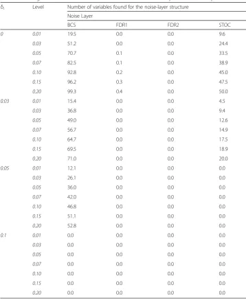
Table 4Average numbers of variables found in the simulation study for the noise-layer structure
δi Level Number of variables found for the noise-layer structure
Noise Layer
BCS FDR1 FDR2 STOC
0 0.01 19.5 0.0 0.0 9.6
0.03 51.2 0.0 0.0 24.4
0.05 70.7 0.1 0.0 33.5
0.07 82.5 0.1 0.0 38.9
0.10 92.8 0.2 0.0 45.0
0.15 96.2 0.3 0.0 47.5
0.20 99.3 0.4 0.0 50.0
0.03 0.01 15.4 0.0 0.0 4.5
0.03 36.8 0.0 0.0 9.4
0.05 49.0 0.0 0.0 12.6
0.07 56.7 0.0 0.0 14.9
0.10 64.7 0.0 0.0 17.5
0.15 69.5 0.0 0.0 18.9
0.20 71.0 0.0 0.0 20.0
0.05 0.01 12.1 0.0 0.0 0.0
0.03 26.1 0.0 0.0 0.0
0.05 36.0 0.0 0.0 0.0
0.07 42.0 0.0 0.0 0.0
0.10 46.8 0.0 0.0 0.0
0.15 51.1 0.0 0.0 0.0
0.20 52.8 0.0 0.0 0.0
0.1 0.01 0.0 0.0 0.0 0.0
0.03 0.0 0.0 0.0 0.0
0.05 0.0 0.0 0.0 0.0
0.07 0.0 0.0 0.0 0.0
0.10 0.0 0.0 0.0 0.0
0.15 0.0 0.0 0.0 0.0
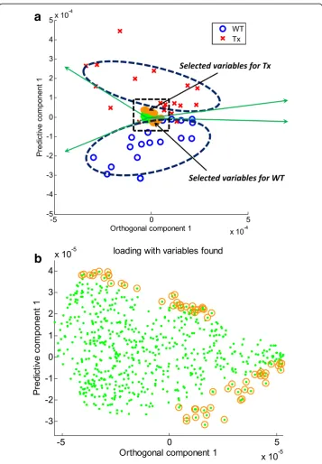
transgenic (TG) mice and wild-type (WT) littermate controls [30]. Thioredoxin (Trx2) is a small protein that regulates reduction-oxidation balance. The chosen dataset com-prised anion exchange-high-resolution mass spectrometry data of mitochondria from 18 WT and 19 TG mice. Metabolic data were extracted from mass spectral analyses using apLCMS [10] and comprised high-resolution m/z features defined by m/z, reten-tion time, and intensity. Each sample was analyzed in duplicate, and data for dupli-cates were averaged. Features with ≥30% missing values were excluded, resulting in 677 features for each sample. The included missing values were replaced by zero since no noticeable peaks at the m/z features were found as in [31]. Comparison of WT and TG data using FDR at q = 0.05 or q = 0.2 resulted in no features being detected as different. Similarly, STOCSYO detected no significant features. Applica-tion of BCR to identify features contributing to the separaApplica-tion of WT and TG mitochondria by the first orthogonal and the first predictive components from OPLS resulted in the identification of 64 features, as shown in Fig. 5 (See also Additional file 7: Table S1).
As post-analysis we annotated the selected metabolites using the Metlin mass spec-trometry database [32]. To determine the associated pathobiology, we applied KEGG (The Kyoto Encyclopedia of Genes and Genomes)-database pathway analysis [33]. Of the 64 features identified by BCR, the 45 had a variable importance projection score≥1 [24]. These 45 discriminatory features were annotated in the Metlin database using
Table 5P-values and classification rates of logistic regression models by detected noise variables
in the noise layers for the three-layer structure
δi Level p-value classification rate
BCS FDR1 FDR2 STOC BCS FDR1 FDR2 STOC
0 0.01 0.0001 0.0001 – – 0.6568 0.6600 – –
0.03 0.0002 0.0002 0.0002 0.0002 0.6578 0.6547 0.6526 0.6563 0.05 0.0004 0.0004 0.0004 0.0004 0.6539 0.6508 0.6481 0.6532
0.07 0.0005 0.0005 – 0.0005 0.6578 0.6537 – 0.6560
0.10 0.0005 0.0005 0.0005 0.0005 0.6710 0.6669 0.6663 0.6691 0.15 0.0004 0.0004 0.0004 0.0004 0.6769 0.6743 0.6739 0.6767 0.20 0.0001 0.0001 0.0002 0.0001 0.6998 0.6979 0.6958 0.6996
0.03 0.01 0.0097 – – – 0.6200 – – –
0.03 0.0006 – – 0.0113 0.6450 – – 0.6150
0.05 0.0000 – – 0.0015 0.7200 – – 0.6300
0.07 0.0000 – – 0.0000 0.8200 – – 0.7000
0.10 0.0000 – – 0.0000 0.8250 – – 0.7100
0.15 0.0000 – – 0.0000 0.7900 – – 0.6650
0.20 0.0000 – – 0.0000 0.8150 – – 0.7700
0.05 0.01 0.0535 – – – 0.6000 – – –
0.03 0.0003 – – – 0.6750 – – –
0.05 0.0001 – – – 0.7150 – – –
0.07 0.0000 – – – 0.6900 – – –
0.10 0.0030 – – – 0.6600 – – –
0.15 0.0000 – – – 0.7550 – – –
only [M + H] + and [M + Na] + adducts (See Additional file 8: Table S2). Twelve of the 45 features were mapped using KEGGMus musculuspathway analysis as shown in Fig.6.
More than two-thirds of the features did not match metabolites in the KEGG data-base, being considered as false positives in practice from the KEGG-database viewpoint. Phosphatidylcholine(18:3) at 518.32 m/z and phosphatidylcholine(18:2) at 520.34 m/z as well as choline phosphate at 184.07 m/z were increased in TG mitochondria compared to WT mitochondria as shown in Figs.6(a) and (d).
Phosphatidylcholine (PC) is one of the most abundant phospholipids as it forms part of the membrane bilayer. Hung et al. investigated the possible role of phosphatidylcholine supplementation as a way of slowing aging-related processes in senescence-accelerated
Fig. 4This figure illustrates selected variables by the four tested methods in the following conditions:ain
layer 1 of the two-layer structure when noise conditionδi= 0 and level = 0.05;bin layer 2 of the
mice [34]. In addition, Al-Orf found that excess and persistent intake of oxidized phosphatidylcholine caused significant damage to organs in male Wistar albino rats [35]. Thioredoxin overexpression in mice has been shown to attenuate oxidative stress [36].
a
b
Fig. 5BCS analysis using orthogonal signal correction of high-resolution metabolomic data from liver
mitochondria from thioredoxin-2 transgenic (TG) mice and wild-type (WT) littermate controls.aA two-dimensional
score plot of orthogonal signal correction shows the first predictive component as a function of the first
orthogonal component.bCorresponding loading plot, a zoomed-in version of the dotted-line rectangle of (a),
with the top 5% of features to the separation of TG and WT metabolic profiles within the 95% correlation range
The discovery of discriminating metabolites related to sphingosine was unantici-pated but reasonable in terms of what is known about ceramide metabolism. Cer-amide is an endogenous mediator of apoptotic cell death. For example, when the intracellular concentration of ceramide is elevated under oxidative stress, cellular proliferation is inhibited, and cellular apoptosis is induced [37]. Ceramide is syn-thesized at the endoplasmic reticulum from palmitoyl-CoA and serine, resulting in 3-ketosphinganine. The enzyme 3-ketosphinganine reductase generates sphinganine from 3-ketosphinganine. Sphinganine is acylated to dihydroceramide by sphinganine N-acyl-transferase. Finally, dihydroceramide is converted to ceramide by the activity of the dihydroceramide desaturase [38–40]. In this study, we observed a reduced amount of 3-ketosphinganine (300.28 m/z) in Trx2-overexpressing TG mice, sug-gesting that Trx2 decreases levels of 3-ketosphinganine, thereby conferring protec-tion against apoptosis (Fig. 7 (b)). Thus, the discrimination of WT and TG mitochondria by 3-ketospingosine is consistent with available data on mitochon-dria, ceramide metabolism, and Trx2 protection against apoptosis signaling.
The discrimination of WT and TG mitochondria by guanosine monophosphate (GMP) at 364.06 m/z is also reasonable because GMP increases antioxidant function and attenuates oxidant cell death [41, 42]. Consistent with the anti-apoptotic effect of GMP, we observed increased GMP in Trx2 TG mice compared to that in WT mice, providing important evidence of overexpression of Trx2 (Fig. 7(c)). The discrimination of WT and TG mitochondria by GMP is consistent with available data on mitochon-dria, the anti-apoptotic effect of GMP on oxidative stress, and Trx2 protection against apoptosis signaling.
Fig. 6Kyoto Encyclopedia of Genes and Genomes (KEGG) pathway analysis of the 45 discriminatory
features identified using the BCS approach. Forty-five discriminatory features are mapped onto 12Mus
Several methods currently exist to identify metabolites that are significantly different according to sample classification based upon the principles of FDR. Comparable methods to test for group behavior of metabolites in sample classification, however, do not exist. Data reduction methods are available to reduce a large number of variables into a smaller set of variables; this allows separation of classes according to the group behavior of metabolites. Previous graphical methods have resulted in identification of individual metabolites that contribute to group behavior; however, no criteria for inclu-sion or excluinclu-sion of metabolites were provided. Our newly developed method, BCR, uses statistical criteria for selection of metabolites contributing to group behavior. Evaluation of its performance with both simulated data and real data demonstrated its utility. The BCR method employs statistical principles to select variables that contribute group-wise to class discrimination. The method allows reproducible selection of metab-olites that contribute to class separation, thereby facilitating practical developments in metabolomics research. Application of BCR could, in principle, provide a simple means to detect group-wise behavior of metabolites connected to different pathways and metabolic networks.
Conclusions
We developed a dimensionality-reduction based approach termed a biplot correlation range that improves reliability of selection of metabolites contributing to group behav-ior for use in metabolic profiling applications for personalized medicine. Original vari-able interactions were used to assign scores according to group identity, and statistical principles were used to select variables in terms of increased score in the direction of a
a
b
c
d
Fig. 7The relative concentrations of mitochondrial metabolites in WT and TG (a) phosphocholine, (b)
group identity within a correlation range. Testing by simulation and application to real data showed that this method improved selection of variables collectively responsible for group behavior. By providing a statistical basis differently from FDR and OPLS--coupled STOCSY approaches, the proposed method can reveal important metabo-lites that contribute to group behavior for analysis of complex metabolic data sets. As a future research direction, more rigorous add-on analysis of selected important metabolites such as the calculation of p-values by cross validation, sensitivity ana-lysis of selection of components, and systemic post-anaana-lysis are in need of investigation.
Additional files
Additional file 1:Figure S1.This figure illustrates selected variables by the four tested methods in the following
conditions: (a) in layer 1 of the one-layer structure when noise conditionδ_i=0.05 and level = 0.05; (b) in layer 2 of
the two-layer structure when noise conditionδ_i=0.05 and level = 0.05; (c) in layer 3 of the three-layer structure
when noise conditionδ_i=0 and level = 0.10; (d) in layer 3 of the two-layer structure when noise condition
δ_i=0.05 and level = 0.10; (e) in the noise layer of the three-layer structure when noise conditionδ_i=0 and level =
0.10; (f) in the noise layer of the one-layer structure when noise conditionδ_i=0.05 and level = 0.05. (DOCX 16 kb)
Additional file 2:Table S1.High-resolution metabolomics features discriminating liver mitochondria from thioredoxin-2 transgenic mice from wildtype littermates as identified by PCLS. (DOCX 16 kb)
Additional file 3:Table S2.Three hundred ten features with variable importance projection (VIP) score greater than and equal to 1 were listed from mitochondria between wild and thioredoxin-2 transgenic mice. (DOCX 16 kb)
Additional file 4:Table S3.P-values and classification rates of logistic regression models by detected noise variables in the noise layers for the two-layer structure. (DOCX 19 kb)
Additional file 5:Table S4.P-values and classification rates of logistic regression models by detected noise variables in the noise layers for the one-layer structure. (DOCX 16 kb)
Additional file 6:Table S5.P-values and classification rates of logistic regression models by detected noise variables in the noise layers for the noise-layer structure. (DOCX 2123 kb)
Additional file 7:Table S6.The average number of filtered variables in each layer and the averaged P-values for the three-layer and two-layer structures from the BCS method. (DOC 75 kb)
Additional file 8:Table S7.The average number of filtered variables in each layer and the averaged P-values for the one-layer and noise-layer structures from the BCS method. (DOCX 58 kb)
Acknowledgements
We would like to thank Jae Ho Cho for his help in reformatting the figures.
Funding
This research was supported by NIH grants S10 OD018006, ES016731, AG038746, ES009047, and ES011195. This research was also supported by the Korea Health Industry Development Institute (grant no. HI14C2686) and the Ministry of Education of the Republic of Korea and the National Research Foundation of Korea (NRF-2017R1D1A1B03032673, NRF-2017M3A9F1031229, NRF-2017R1A2B4003890). This research was also supported by the grant (S2652960) funded by Ministry of SMEs and Startups and TIPA in the Republic of Korea.
Availability of data and materials
The implemented MATLAB package is available from the following url addresses:
https://github.com/kongktw/BCR,https://zenodo.org/record/2432975#.XBq1HFxKjmg.
Authors’contributions
YHP performed metabolic analyses on the experimental data and participated in the writing of the manuscript. JRR provided the experimental data and biological analyses on the experimental data. TK performed analyses on the simulated data helped finalizing the manuscript. DPJ motivated the research problem and designed the study. KL implemented the algorithms and drafted the manuscript. All authors read and approved the final manuscript.
Competing interest
The authors declare that they have no competing interests.
Ethics approval and consent to participate Not applicable.
Competing interests
The authors declare that they have no competing interests.
Publisher’s Note
Springer Nature remains neutral with regard to jurisdictional claims in published maps and institutional affiliations.
Author details
1
College of Pharmacy, Korea University, Sejong 30019, South Korea.2Industrial and Systems Engineering, Georgia Institute of Technology, Atlanta, GA 30332, USA.3Skaggs School of Pharmacy and Pharmaceutical Sciences, University
of Colorado, Denver, CO 80045, USA.4Clinical Biomarkers Laboratory, Division of Pulmonary, Allergy and Critical Care Medicine, Atlanta, GA 30322, USA.5Department of Medicine, Emory University, Atlanta, GA 30322, USA.6Department of
Industrial Engineering, Hanyang University, Seoul 04763, South Korea.
Received: 12 June 2018 Accepted: 10 January 2019
References
1. Jonsson P, et al. Extraction, interpretation and validation of information for comparing samples in metabolic LC/MS data
sets. Analyst. 2005;130(5):701–7.
2. Soltow QA, et al. High-performance metabolic profiling with dual chromatography-Fourier-transform mass spectrometry
(DC-FTMS) for study of the exposome. Metabolomics. 2011.
3. Garcia A, Barbas C. Gas chromatography-mass spectrometry (GC-MS)-based metabolomics. Methods Mol Biol. 2011;708:
191–204.
4. Tsugawa H, et al. Practical non-targeted gas chromatography/mass spectrometry-based metabolomics platform for
metabolic phenotype analysis. J Biosci Bioeng. 2011;112:292–8.
5. Park Y, et al. Individual variation in macronutrient regulation measured by proton magnetic resonance spectroscopy of
human plasma. Am J Physiol Regul Integr Comp Physiol. 2009;297(1):R202–9.
6. Serkova NJ, Niemann CU. Pattern recognition and biomarker validation using quantitative 1H-NMR-based metabolomics.
Expert Rev Mol Diagn. 2006;6(5):717–31.
7. Nicholson JK, Lindon JC. Systems biology: metabonomics. Nature. 2008;455(7216):1054–6.
8. Smilde AK, Westerhuis JA, Hoefsloot HCJ, Bijlsma S, Rubingh CM, Vis DJ, Jellema RH, Pijl H, Roelfsema F, van der Greef J.
Dynamic metabolomic data analysis: a tutorial review. Metabolomics. 2010;6(1):3–17.
9. Weis BK, Balshaw D, Barr JR, Brown D, Ellisman M, Lioy P, Omenn G, Potter JD, Smith MT, Sohn L, et al. Personalized exposure
assessment: promising approaches for human environmental health research. Environ Health Perspect. 2005:840–8.
10. Yu T, et al. apLCMS--adaptive processing of high-resolution LC/MS data. Bioinformatics. 2009;25(15):1930–6.
11. Uppal K, et al. xMSanalyzer: automated pipeline for improved feature detection and downstream analysis of large-scale,
non-targeted metabolomics data. BMC Bioinformatics. 2013;14:15.
12. Benjamini Y, Hochberg Y. Controlling the false discovery rate: a practical and powerful approach to multiple testing. J R
Statist Soc B. 1995;B57:289–300.
13. Loscalzo J, Kohane I, Barabasi AL. Human disease classification in the postgenomic era: a complex systems approach to
human pathobiology. Mol Syst Biol. 2007;3:124.
14. Moriarty-Craige SE, Ha KN, Sternberg P Jr, Lynn M, Bressler S, Gensler G, Jones DP. Effects of long-term zinc
supplementation on plasma thiol metabolites and redox status in patients with age-related macular degeneration. Am J
Ophthalmol. 2007;143(2):206–11.
15. Ha KN, Chen Y, Cai J, Sternberg P Jr. Increased glutathione synthesis through an ARE-Nrf2--dependent pathway by zinc
in the RPE: implication for protection against oxidative stress. Invest Ophthalmol Vis Sci. 2006;47(6):2709–15.
16. Gabory A, Attig L, Junien C. Epigenetic mechanisms involved in developmental nutritional programming. World J
Diabetes. 2011;2(10):164–75.
17. Lillycrop KA, Burdge GC. The effect of nutrition during early life on the epigenetic regulation of transcription and
implications for human diseases. J Nutrigenet Nutrigenomics. 2012;4(5):248–60.
18. Alvin CR Methods of multivariate analysis. 2002, Wiley Interscience. P. 531.
19. Cloarec O, et al. Statistical total correlation spectroscopy: an exploratory approach for latent biomarker identification
from metabolic 1H NMR data sets. Anal Chem. 2005;77(5):1282–9.
20. Greenacre, Michael J, Biplots in practice,Fundacion BBVA, 2010.
21. Gower, John C and Lubbe, Sugnet Gardner and Le Roux, Niel J, Understanding biplots,John Wiley \& sons, 2011.
22. Greenacre MJ. Biplots: the joy of singular value decomposition. Wiley Interdisciplinary Reviews: Computational Statistics.
2012;4(4):399–406.
23. Westerhuis JA, et al. Direct orthogonal signal correction. Chemom Intell Lab Syst. 2001;56(1):13–25.
24. Eriksson L, Johansson E, Kettaneh Wold N, Wold S. Multi and Megavariate Data Analysis; Umetrics AB, Umeå, Sweden,
2001.
25. Jones DP, Park Y, Ziegler TR. Nutritional metabolomics: Progress in addressing complexity in diet and health. Annu Rev
Nutr. 2012;21(32):183–202.
26. Kinross JM, et al. Global metabolic phenotyping in an experimental laparotomy model of surgical trauma. J Proteome
Res. 2010;10:277–87.
27. Lindon JC, Nicholson JK. Spectroscopic and statistical techniques for information recovery in metabonomics and
metabolomics. Annu Rev Anal Chem (Palo Alto Calif). 2008;1:45–69.
28. Benjamini Y, Yekutieli D. The control of the false discovery rate in multiple testing under dependency. Ann Stat. 2001:
29. Holmes E, Cloarec O, Nicholson JK. Probing latent biomarker signatures and in vivo pathway activity in experimental disease states via statistical total correlation spectroscopy (STOCSY) of biofluids: application to HgCl2 toxicity. J
Proteome Res. 2006;5(6):1313–20.
30. Roede JR, et al. Detailed mitochondrial phenotyping by high resolution metabolomics. PLoS One. 2012;7(3):e33020.
31. Xia J, et al. MetaboAnalyst: a web server for metabolomic data analysis and interpretation. Nucleic Acids Res. 2009;37:
W652–60.
32. Smith CA, et al. METLIN: a metabolite mass spectral database. Ther Drug Monit. 2005;27(6):747–51.
33. Kanehisa M, et al. The KEGG databases at GenomeNet. Nucleic Acids Res. 2002;30:42–6.
34. Hung MC, et al. Learning behaviour and cerebral protein kinase C, antioxidant status, lipid composition in
senescence-accelerated mouse: influence of a phosphatidylcholine-vitamin B12 diet. Br J Nutr. 2001;86(2):163–71.
35. Al-Orf SM. Effect of oxidized phosphatidylcholine on biomarkers of oxidative stress in rats. Indian J Clin Biochem. 2011;
26(2):154–60.
36. Li GX, et al. Thioredoxin overexpression in mice, model of attenuation of oxidative stress, prevents benzene-induced
hemato-lymphoid toxicity and thymic lymphoma. Exp Hematol. 2006;34(12):1687–97.
37. Gudz TI, Tserng KY, Hoppel CL. Direct inhibition of mitochondrial respiratory chain complex III by cell-permeable
ceramide. J Biol Chem. 1997;272(39):24154–8.
38. Cuvillier O. Sphingosine in apoptosis signaling. Biochim Biophys Acta. 2002;1585(2–3):153–62.
39. Henry B, et al. Targeting the ceramide system in cancer. Cancer Lett. 2013;332(2):286–94.
40. Levade T, et al. Ceramide in apoptosis: a revisited role. Neurochem Res. 2002;27(7–8):601–7.
41. Polte T, Oberle S, Schroder H. Nitric oxide protects endothelial cells from tumor necrosis factor-alpha-mediated
cytotoxicity: possible involvement of cyclic GMP. FEBS Lett. 1997;409(1):46–8.
42. Stephens RS, et al. cGMP increases antioxidant function and attenuates oxidant cell death in mouse lung microvascular