R E S E A R C H A R T I C L E
Open Access
An automatic restoration framework based
on GPU-accelerated collateral filtering in
brain MR images
Herng-Hua Chang
*and Cheng-Yuan Li
Abstract
Background:Image restoration is one of the fundamental and essential tasks within image processing. In medical imaging, developing an effective algorithm that can automatically remove random noise in brain magnetic resonance (MR) images is challenging. The collateral filter has been shown a more powerful algorithm than many existing methods. However, the computation of the collateral filter is more time-consuming and the selection of the filter parameters is also laborious. This paper proposes an automatic noise removal system based on the accelerated collateral filter for brain MR images.
Methods:To solve these problems, we first accelerated the collateral filter with parallel computing using the graphics processing unit (GPU) architecture. We adopted the compute unified device architecture (CUDA), an application programming interface for the GPU by NVIDIA, to hasten the computation. Subsequently, the optimal filter parameters were selected and the automation was achieved by artificial neural networks.
Specifically, an artificial neural network system associated with image feature analysis was adopted to establish the automatic image restoration framework. The best feature combination was selected by the paired t-test and the sequential forward floating selection (SFFS) methods.
Results:Experimental results indicated that not only did the proposed automatic image restoration algorithm perform dramatically faster than the traditional collateral filter, but it also effectively removed the noise in a wide variety of brain MR images. A speed up gain of 34 was attained to process an MR image, which completed within 0.1 s. Representative illustrations of brain tumor images demonstrated the capability of identifying lesion boundaries, which outperformed many existing methods.
Conclusions:We believe that our accelerated and automated restoration framework is promising for achieving robust filtering in many brain MR image restoration applications.
Keywords:Collateral filter, GPU, Parallel computing, Image feature, Neural networks, MRI
Background
Since its invention in the 1970s, magnetic resonance imaging (MRI) has been an important imaging technique for noninvasive diagnosis of the human body. The appli-cations of MRI in the brain result in diversified images for further processes such as tissue classification, seg-mentation and registration [1–3]. However, the random noise in MRI scanners inevitably causes deterioration of
brain MR images [4]. Consequently, noise removal has become a crucial issue in brain MR image post-processing [5]. The Gaussian filter has been extensively adopted in many image processing applications for its simplicity. However, anatomical boundaries are inevitably blurred by this lowpass filter. In addition to the Gaussian filter, one of the well-known techniques for noise removal has been the bilateral filter, which was originally proposed by Tomasi and Manduci [6]. It has been widely utilized in many med-ical image denoising applications for decades. The bilateral filter is an effective filtering algorithm that can both remove the random noise and preserve edges rather than * Correspondence:[email protected]
Computational Biomedical Engineering Laboratory (CBEL), Department of Engineering Science and Ocean Engineering, National Taiwan University, No. 1 Sec. 4 Roosevelt Road, Daan, 10617 Taipei, Taiwan
blurring the lines in images. An iterative version of the bilateral filter for MR image restoration was recently introduced [7].
One remarkable technique of using statistics strategies is the linear minimum mean squared error (LMMSE) estimator [8], which computes the local mean, the local variance, and the local mean square value of the input image. Another famous method is the anisotropic diffu-sion filter (ADF) [9], in which pixel intensities are aver-aged from neighbors in a prescribed window, whose dimension and shape are measured at every location. An appropriate function of the image gradient is con-structed in accordance with the diffusion coefficient to encourage filtering within a region of interest in prefer-ence not to filtering across the boundaries. It is noted that the quality of the denoised image is greatly relevant to the number of iterations. Subsequently, Ferrari [10] proposed a mathematical framework to automatically determine the best number of iterations of the ADF method by utilizing the maximization of some evalu-ation index. Nevertheless, it has been adopted in many medical image restoration applications [11].
In contrast to many methods that mainly reply on local pixels within a small neighbourhood, the non-local means (NLM) filter detects repeated structures in the global domain [12]. The similarity between pixels is region-based comparison in that pixels far from the ker-nel center are not penalized due to the distance to the center. Based on an enhanced sparse representation in the transform domain, the block-matching and 3D filter-ing (BM3D) strategy [13] extended the nonlocal filtering techniques. The enhancement of the sparsity is accom-plished by aggregating similar 2D fragments of the image into 3D arrays. Subsequently, the Wiener filter is employed in the collaborative filtering procedure to remove noise.
Motivated by the bilateral filter, the collateral filter [14] was recently proposed that introduced a median filter and an entropy function to the filtering frame-work. The median filter compensated the Gaussian fil-ter for random noise reduction. It has been shown that the collateral filter is more powerful than the Gaussian filtering, bilateral filtering, and ADF methods in many scenarios [14]. However, comparing to these two filters, the collateral filter is more complicated and time con-suming. A contemporary technique called the tensor processing unit (TPU) has shown its excellent compu-tation and energy efficiency over existing frameworks [15]. However, this domain specific architecture is ex-clusively deployed in Google data centers. One realistic approach to speed up the denoising procedure is through the parallel programming using the compute unified device architecture (CUDA) [16, 17] with the graphics processing unit (GPU).
A GPU is a specialized processor that accelerates graphic operations on personal computers, workstations, and mobile devices. The GPU has more processor cores than a traditional central processing unit (CPU) and each core can process data simultaneously. Therefore, the GPU is well suited to handle tasks that can be paral-lelized. For example, GPU-based acceleration has been shown effective in segmentation and classification appli-cations [18, 19]. Additionally, CUDA is a programming platform developed by NVIDIA for general purpose computation on GPU (GPGPU) on NVIDIA GPUs [20]. Many of NVIDIA graphics cards support CUDA (e.g., GeForce, Quadro, and Tesla). With CUDA, program-mers can manage memory on the CPU as well as the GPU from the host. Once memory spaces on both host and device sides are allocated and data are trans-ferred, the program can launch kernels for execution on the device.
A kernel is a function that can be called from the host and executed on the device. Programmers can design the code in the kernel function for parallel computing. The kernel function defines the operations for a single thread and thousands of threads execute the function code synchronously. A thread is the basic execution unit for parallel computing. After the thread completes its task in the kernel function, the data are transferred back to the host.
Based on the GPU architecture, one pixel in an image can be handled by one thread and thousands of threads can run synchronously. Each thread can access data from different types of memories such as local, global and shared memory. While local memory be-longs to one specific thread, global memory is shared by all threads. Indeed, local memory is part of global memory and both is slower than shared memory. Threads are organized in blocks and a grid is a group of blocks. Each block has its shared memory that can be accessed by its own threads. Although shared mem-ory’s size is smaller than global memory, the access time of shared memory is faster like cache [21].
The objective of this paper is two-fold. First, to accel-erate the computation of the collateral filter through the adoption of the CUDA strategy. Second, to automate the collateral filtering process by the aid of image texture features associated with artificial neural networks [22]. We will show that a fast and automatic denoising system based on CUDA-based collateral filtering provides robust and accurate restoration results over many existing denoising methods.
Methods
CUDA-based collateral filtering
that it contains three different Gaussian functions [14]. Let (θx,θy) be the pixel location under consideration in the filtering image and Ψθx;θy be the neighborhood of (θx,θy):
Ψθx;θy¼ μx;μy
:ðμx;μyÞ∈½θx−N;θxþN ½θy−N;θyþN
n o
ð1Þ
where Nis the filter radius. The Gaussian functions for the spatial, radiometric and median-filtered components are respectively defined as
WSθx;θy μx;μy
¼ exp − μx;μy
−ðθx;θyÞ
2
2σ2 S 2 6 4 3 7 5 ð2Þ
and
WRθx;θy μx;μy
¼ exp − I μx;μy
−Iðθx;θyÞ
2
2σ2 R 2 6 4 3 7 5
ð3Þ
and
WMθx;θy μx;μy
¼ exp − I
M μ
x;μy
−IMðθx;θyÞ
2
2σ2 M 2 6 4 3 7 5
ð4Þ
where I(μx,μy)is the intensity value at(μx,μy) and
IM(μx,μy) is the median filtered image at location (μx,μy). In addition to median filtering, the collateral filter introduces an entropy function that is utilized to balance the radiometric and median-filtered com-ponents using
H θx;θy
¼−X μ
x;μy
ð Þ∈Ψθx;θyp μx;μy
logp μx;μy
þ 1−p μx;μy
h i
log 1−p μx;μy
h i
ð5Þ
where
p μx;μy
¼
1−jIðμx;μyÞ−IMðμx;μyÞj
MAXI
2
2 þ0:5 ð6Þ
where MAXI is the maximum intensity value of the input imageI.
The ensemble weight function that combines all the components is then defined as
Wθx;θy ¼W
S θx;θy W
R θx;θy
1
1þHðθx;θyÞ WMθx;θy
Hðθx;θyÞ ð7Þ
The collateral filtering of image Iat location(θx,θy) is finally computed using
IC θx;θy
¼ P
μx;μy
ð Þ∈ΨWθx;θy μx;μy
1−β
ð ÞIþβIM P
μx;μy
ð Þ∈ΨWθx;θy μx;μy
ð8Þ
where β is adopted to adjust the weight between the input imageIand the median filtered imageIM. A num-ber of techniques have been proposed to accelerate image filter computation. Some researchers used approximation methods to reduce the computation time [23]. A straightforward approach is to take advantage of an additional memory space. Inspired by the strategy in [24], we introduce a new scheme not only saving com-putation time but also achieving the same restoration re-sults as using the traditional collateral filter.
In the traditional collateral filter, the spatial compo-nent is repeatedly computed for every pixel, which takes a lot of time in computing the same pixel distances. Therefore, we redefine (2) as
DS dx;dy
¼ exp −dx
2þ
dy2
2σ2 S
ð9Þ
wheredx anddyare the spatial distances with 0≤dx≤N and 0≤dy≤N. In our approach, we create a spatial weight bufferWSB, which is defined as
WSB¼ DS dx;dy
:dx;dy∈½1;…;N
ð10Þ
We then compute all the spatial weights and store them in this memory bufferWSB according to the filter radius N. Let WSB(x,y) be an element of WSB, (2) can be expressed asWSB(μx−θx,μy−θy).
Subsequently, we implement the complex parts of the collateral filter using CUDA shared memory, which is an efficient way to reduce the reading and writing time comparing to the usage of global memory. We split the image pixels into separate blocks, each denoted as block(i, j), where i= 1, 2, …, k and j= 1, 2, …, k. For entropy computation, each pixel and its neighbors are required to sum up as shown in (5). To hasten the com-putation, the entropy of the pixel at (x, y) is computed and stored in the shared memory buffer in advance using
HPBi;jðx;yÞ ¼p xð ;yÞlogp xð ;yÞ
þ½1−p xð ;yÞlog 1½ −p xð ;yÞ
ð11Þ
S×j+N, andS×Srepresents the block size. OnceHPBi, jis created, the entropy is defined as:
HGi;j δx;δy
¼−X μ
x;μy
ð Þ∈Ψδx;δyHPBi;j μx;μy
ð12Þ
where (δx,δy) represents a thread in block(i,j) with 1≤δx≤
Sand 1≤δy≤S. Since accessing shared memory is faster than accessing local memory, each thread only needs to sum up its own value from its neighbors. Consequently, we redefine (7) as:
Wi;j;δx;δy¼WSBi;j WRi;j;δx;δy
1
1þHGi;jðδx;δyÞ
WM
i;j;δx;δy
HGi;jðδx;δyÞ
ð13Þ
where WSBi, j represents the spatial weight buffer in block(i,j).
In order to more effectively utilize shared memory, the computation ofβin (8) is reformulated so that it is cal-culated at the beginning in every block(i,j) before apply-ing the filter to each pixel. Finally, the accelerated version of the collateral filter is defined as:
IAC i;j δx;δy
¼
P
μx;μy
ð Þ∈Ψδx;δyWi;j;δx;δy μx;μy
BETAi;j μx;μy
P
μx;μy
ð Þ∈Ψδx;δyWi;j;δx;δy μx;μy
ð14Þ
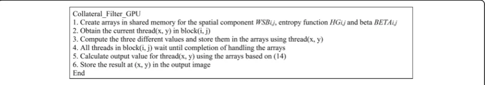
where BETAi, j(μx,μy) is the value of β at (μx,μy). The pseudo code of our GPU-based collateral filter is depicted in Fig.1. Note that each pixel being processed is assigned to a thread since the process is a slice-by-slice approach, i.e., one 2D image at a time.
Feature extraction
Although the execution time of the traditional collateral filter is hastened using the GPU strategy, it is still labori-ous to manually adjust the parameters for achieving the best restoration results in a particular brain MR image. Using an artificial neural network system is suitable as it can learn to estimate the optimal parameters in the fil-tering process. However, neural networks require appro-priate input features to obtain the best performance of the predictable model. In our experience, image texture
features play an important role in the neural network automation process. The candidate image texture fea-tures adopted in this study are described as follows.
Statistical features
There are several basic statistical features that are com-puted directly from the image intensity: mean intensity (Mean), standard deviation (SD), variance (VAR), entropy (ENT), and histogram features (skewness, kurtosis, vari-ance, entropy and energy).
Gray-level co-occurrence matrix (GLCM)
The GLCM features were proposed by Haralick et al. [25]. A co-occurrence matrix is defined as a matrix of frequencies at which two pixels, separated by a certain distance and direction, occur in the image. Eight GLCM features [25–27] in four directions (θ=0°, 45°, 90°, 135°) with distanced =1 are computed:
(1) Standard deviations in thei-direction (SDi) (2) Standard deviations in thej-direction (SDj) (3) Energy or angular second moment (ASM) (4) Contrast (CON)
(5) Dissimilarity (DIS) (6) Homogeneity (HOM) (7) Entropy (ENT) (8) Correlation (COR)
Gray-level run-length matrix (GLRLM)
The GLRLM features were proposed by Galloway [28]. A run-length matrix is defined as the number of runs with a pixel of a specific gray level and its run length in a certain direction. Eleven GLRLM features in four directions (θ= 0°, 45°, 90°, 135°) are computed:
(1) Short run emphasis (SRE) (2) Long run emphasis (LRE) (3) Gray level nonuniformity (GLN) (4) Run length nonuniformity (RLN) (5) Run percentage (RP)
(6) Low gray-level run emphasis (LGRE) (7) High gray-level run emphasis (HGRE) (8) Short run low gray-level emphasis (SRLGE)
(9) Short run high gray-level emphasis (SRHGE) (10)Long run low gray-level emphasis (LRLGE) (11)Long run high gray-level emphasis (LRHGE)
Tamura texture features
Tamura features [29] were developed based on the human visual and psychological perception. The first three features, which are correlated more closely with human perception, are computed:
(1) Coarseness (CRS) (2) Contrast (CON) (3) Directionality (DIR)
Their formulas are briefly provided in Additional file1.
Noise estimation features
Since the collateral filter parameters are sensitive to noise, noise related features are required. Many noise variance estimation methods that are based on the Rician and Rayleigh distributions are complicated. An easier way to estimate the noise level is to employ a sim-pler Laplacian operator [30]. A more efficient algorithm [31] with a generic transfer function improved the Laplacian mask for better estimation. Aja-Fernández et al. [32] presented a set of estimators based on the Ray-leigh distribution in the background. Moreover, the peak value of the autocorrelation function computed by an image with itself provides the information of noise [33]. Based on the above methods, the following seven fea-tures are adopted:
(1) Laplacian mask (LAP) (2) Laplacian of Gaussian (LOG)
(3) A generic transfer function with Laplacian (GTFLAP)
(4) Maximum value of some local distribution (AJA) (5) A least square fitting of the Rayleigh distribution
with the histogram background (BRUM) (6) Maximum likelihood function (SIJ) (7) Autocorrelation function (ACF)
Feature selection
If a large amount of features are selected as the input arguments, the training of neural networks will be an extremely time-consuming procedure. Consequently, we utilize the sequential forward floating selection (SFFS) method [34] to choose the best combination of features. Before applying the SFFS, we make use of the paired-samples t-test [35,36] to rank the significance of candidate features. The t-test is applied to each image feature to evaluate the ability for discriminating differ-ences between noise levels, which results in an average
p-value. The smaller the p-value, the better the
discrimination. Statistically, those features with an average p< 0.05 are selected as candidates for the SFFS process.
Neural networks
The popular back propagation neural network (BPN), proposed by McClelland et al. [37], is utilized for train-ing our neural network system. The main architecture includes input, hidden and output layers. The back propagation process is employed to optimize the weights by minimizing the target error so that the neural net-work is able to learn the input-output mapping perfectly. In our approach, the inputs are the features selected by the SFFS algorithm and the outputs are the collateral fil-ter paramefil-ters. In addition, a brute-force approach is conducted to obtain the optimal filter parameters based on the peak signal-to-noise ratio (PSNR):
PSNR¼10 log10 MAX
2 I
1
mn
X m−1
i¼0 Xn−1
j¼0
R ið Þ;j −Fði;jÞ
½ 2
2 6 6 6 6 4
3 7 7 7 7 5
ð15Þ
where F is the m×n noise-free image, Ris the restored image, andMAXIis the maximum possible intensity ofF.
The optimal filter parameters are decided when the highestPSNRvalue is obtained.
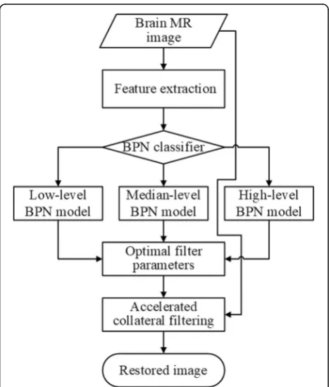
Finally, a two stage neural network structure is developed with the first stage for classification and the second stage for prediction. At the first stage, the neural network classifier distinguishes inputs into three differ-ent noise levels. Multiple-layer (input, hidden, and out-put) neural networks with different noise level models at the second stage predict the optimal filter parameters for image restoration. The Levenberg-Marquardt learn-ing algorithm [38] is exploited to independently train each of the three individual BPN models. For each BPN model, the transfer function between the input layer and the hidden layer is the hyperbolic tangent function, whereas the linear transfer function is employed between the hidden layer and the output layer. The overall flow-chart of the proposed methods is depicted in Fig.2.
Performance evaluation
In addition to the PSNR metric in (15), the structural similarity (SSIM) metric [39] is utilized to evaluate the restored images using
SSIMðF;RÞ ¼ μ2ð2μFμRþC1Þð2σFRþC2Þ
Fþμ2RþC1
σ2
Fþσ2RþC2
ð16Þ
where σ represents the standard deviation, μ represents the mean intensity,C1= (K1MAXI)
2
and C2= (K2MAXI) 2
with K1= 0.01 and K2= 0.03. The higher the PSNR and SSIM scores the better the restoration results. To more thoroughly evaluate the image restoration ability of the proposed system, the restoration results obtained using the automatic framework are compared with the results obtained using the brute-force method, which is consid-ered as the optimal outcome. Let PSNRAbe the restor-ation score of the proposed automatic system and
Table 1Execution time of the CPU-based and GPU-based collateral filters
Image number
CPU (s)
GPU without SM (s)
GPU with SM (s)
Speed up
1 0.63 0.14 0.018 34
10 6.06 0.16 0.027 224
100 58.78 0.24 0.108 541
500 260.52 0.59 0.425 612
1000 512.38 1.05 0.871 588
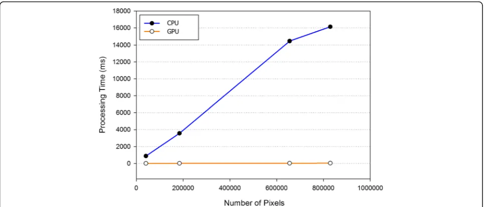
Fig. 3Plots of the running times of the CPU-based and the GPU-based with shared memory collateral filters
Table 2Paired-samples t-test results based on the average
p-value withp< 0.05
No. Feature p-value No. Feature p-value
1 BRUM 0.019017 15 AJA 0.038044
2 SIJ 0.020022 16 GLN(45°) 0.038485
3 SRLGE(90°) 0.021380 17 RP(45°) 0.040108
4 GTFLAP 0.022898 18 RP(135°) 0.040233
5 SRLGE(45°) 0.023014 19 LGRE(0°) 0.041105
6 SRLGE(0°) 0.028114 20 LGRE(90°) 0.041233
7 SRLGE(135°) 0.028445 21 RLN(135°) 0.042278
8 RLN(90°) 0.030137 22 SIJ 0.043803
9 GLN(0°) 0.032553 23 LAP 0.044592
10 RP(0°) 0.032900 24 LGRE(135°) 0.045512
11 RP(90°) 0.033309 25 GLN(135°) 0.046477
12 GLN(90°) 0.033748 26 RLN(45°) 0.046907
13 RLN(0°) 0.034005 27 ACF 0.048627
PSNRT be the restoration score of the brute-force method. The relative errorεris then defined as
εr¼
PSNRT−PSNRA
j j
PSNRT
100% ð17Þ
Results
We first conducted the experiments on the BrainWeb database [40] as it contains simulated brain MR image data based on normal and multiple sclerosis (MS) models with different thicknesses, noise levels and intensity non-uniformities. Clinical image data
were acquired from the medical image database in the Division of Interventional Neuro Radiology, Department of Radiology, UCLA, Los Angeles, CA, USA. For efficiency tests, the experiments were per-formed on an Intel® Xeon(R) CPU E5–2620 v3 2.40GHz equipped with a Tesla K40c GPU. Tesla K40c is one NVIDIA’s GPU based on the NVIDIA’s Kepler architecture. The Tesla K40c GPU contains 15 multiprocessors and each multiprocessor contains 192 cores, which results in 2880 cores. Its memory size is 12 GB and the maximum bandwidth is 288 (GB/sec). Each block has 65,536 registers with 48 KB shared memory and the maximum number of threads is 1024. The CUDA driver version is 7.5. The algorithm was implemented and programmed in MATLAB 2017a (The MathWorks Inc. Natick, MA, USA) asso-ciated with C for CUDA-based acceleration.
Table 1 presents the execution performance of the traditional collateral filter and our accelerated version on the same 217 × 181 brain MR images. The performance of using the shared memory (SM) or not is also indi-cated. The block size for the shared memory was 16 × 16 threads and the filter size was 3 × 3. When the number of images was increasing, the proposed framework exe-cuted the filtering process more effectively and a remarkable acceleration was attained. It was noted that
Table 3Restoration result analyses of the proposed GPU-based collateral filter on different slices
Slice 7 14 17 20 23
Noise
5% PSNRA 33.066 34.131 34.156 33.836 34.736
PSNRT 33.229 34.145 34.157 33.855 34.758
εr(%) 0.4891 0.0395 0.0031 0.0575 0.0621
7% PSNRA 31.278 31.728 31.956 32.015 32.613
PSNRT 31.355 31.837 31.960 32.028 32.658
εr(%) 0.2453 0.3430 0.0117 0.0415 0.1377
the speed up gain raised from 34 for one single image to 541 for processing 100 images. Our proposed GPU-based collateral filter is much faster than the ori-ginal CPU version. The corresponding running times with respect to different image pixel sizes are depicted in Fig. 3. Obviously, the GPU implementation ran less than 0.1 s for each scenario, whereas the computation time of the CPU version was roughly linearly propor-tional to the pixel number.
As presented in Table 2, there were 28 selected fea-tures from different image feature classes for the input candidates of the BPN system. The order of significance of these adopted image features was based on the aver-age p-value of the t-test outcome with p< 0.05. For understanding the optimal features, T1-weighted brain MR images with three different slice thicknesses (1 mm, 3 mm and 5 mm), five noise levels (1, 3, 5, 7 and 9%), and three intensity non-uniformities (0, 20 and 40%) acquired from the BrainWeb database were utilized to evaluate the proposed automatic restoration framework. Each noise level had 1476 images, which were divided into two groups: 984 slices for training and 492 slices for testing. After the SFFS procedure, five optimal features of RLN(0°), RP(135°), RP(90°), AJA, and kurtosis were obtained and they were further employed in the BPN training phase.
In the testing phase, the first stage BPN system classi-fied the input image into three major categories based on the noise level: low (1 and 3%), median (5 and 7%) and high (9%) estimators. The correct classification rate was up to 97.6% overall. The computed five features of the input image were fed into the corresponding second stage BPN model for producing the filter parameter values for denoising. Table 3 summarizes the PSNR scores and the relative error εr of the proposed auto-matic filtering framework and the brute-force method on randomly selected slices of the 5 mm normal MR im-ages with 5 and 7% noise. It is indicated that the PSNR scores of the proposed restoration algorithm were extremely close to the optimal PSNR scores of the brute-force method with negligible errors.
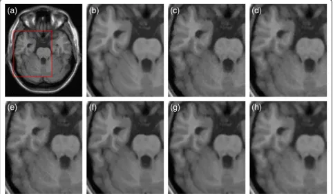
In Fig. 4, we illustrate our automatic restoration out-come of the 10th slice image corrupted by 5% noise level in the 5 mm MS dataset in comparison with the ADF [9], LMMSE [8], NLM [12], iterative bilateral filtering (IBF) [7], and BM3D [13] methods. Comparing to other techniques, the proposed GPU-based collateral filter re-vealed more uniform intensity profiles and better sharp-ened edges in the white matter (WM) and gray matter (GM) regions. Quantitative analyses also indicated that our automatic collateral filter provided the highest score of PSNR = 34.32 dB and the second highest SSIM =
0.8803 than other tested methods. Figure 5 depicts the visual restoration results of the 26th slice image cor-rupted by 7% noise level in the 3 mm MS dataset. It was obvious that, in contrast to other methods, the proposed denoising algorithm achieved a sharper and cleaner rep-resentation for the GM and WM with the best PSNR = 31.95 dB and SSIM = 0.8479, which was closer to the intact image.
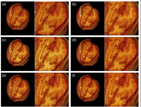
Figure6delineates the restoration results of the 1 mm normal image volume with 9% noise level and 40% in-tensity non-uniformity in 3D visualization. After apply-ing the ADF, LMMSE, and IBF methods, the brain structures still, more or less, exhibited grainy noise influ-ences. On the other hand, the proposed automatic filter decently wiped out the heavy noise while maintaining noticeable cortical structures as illustrated in Fig. 6f. Table 4 presents quantitative analyses on massive 1 mm image volume restoration with various scenarios of ana-tomical models and noise levels. It was noted that the LMMSE method performed much worse than other
methods in the image volumes with 1% noise. Our auto-matic denoising framework produced the best restor-ation results in terms of average PSNR and SSIM in all noise levels. As the noise level was increasing, the advantage of our collateral filter over other methods was more compelling.
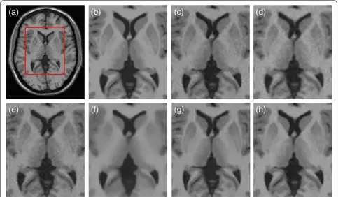
For completeness, we demonstrate the capability of our automatic filtering algorithm in restoring clinical brain MR images with diseases. Figure7depicts the res-toration results of denoising T1-weighted MR images with brain tumors using different methods. While the restoration results obtained using the ADF, LMMSE, and IBF methods were somewhat grainy in the tumor area, the NLM, BM3D and proposed algorithms achieved more suitable smoothness while maintaining sharpness at the tumor boundaries. Another example of filtering distorted PD-weighted MR images with brain tumors is illustrated in Fig.8. It was indicated that, com-paring to other methods, our automatic collateral filter more effectively removed the artefact while disclosing
distinct edges between anatomical structures. Finally, in Fig. 9, we show the visual improvement of noisy MR images with low resolution and severe grains using all tested methods. It was obvious that the proposed filter-ing algorithm more adequately eliminated the noise and identified the lesion in contrast to other techniques.
Discussion
Stimulated by the recent advance in artificial intelligence and parallel computing, we have devel-oped an efficient filtering framework for brain MR
images. An essential property of the proposed auto-matic restoration algorithm is the two-stage mechan-ism of the neural network concatenation. A benefit of this strategy is to divide the broad noise range into three narrower classes corresponding to three individ-ual BPN models, where the prediction of the filter pa-rameters can be further clarified. To correlate the image with the BPN models for automation, a wide variety of image texture features were investigated based on the SFFS strategy, from which five best texture features were obtained. Three features of RLN(0°), RP(135°), and RP(90°) belong to the GLRLM category, AJA is one of the noise estimation features, and kurtosis makes use of the histogram information. These five features play an essential role in the effect-ive discrimination between images with different noise levels, anatomical structures, and intensity non-uniformities.
A variety of T1-weighted brain MR images acquired from the BrainWeb database [40] with various scenarios were utilized in the proposed BPN models to obtain the optimal filter parameters. Due to the facility limitations, other MR modalities such as T2-weighted and PD-weighted images were not included in the training dataset in the current study. From the viewpoint of the clinical demand, the proposed automatic filter adequately restored various brain MR images with dis-tinct anatomical structures and modalities such as PD-weighted images (see Figs. 7,8,9), which were quite
Fig. 7Comparison of the restoration of clinical T1-weighted MR images with brain tumors.aInput MR image.bInput image in magnified view. cIBF.dADF.eLMMSE.fNLM.gBM3D.hProposed
Table 4Quantitative analyses on the restoration results of the 1 mm image data in terms of average PSNR and SSIM scores using different methods
Type Noise LMMSE IBF Proposed
PSNR SSIM PSNR SSIM PSNR SSIM
Normal 1% 34.97 0.8513 38.04 0.9766 39.17 0.9816
3% 33.34 0.8626 33.28 0.8924 34.79 0.9027
5% 30.65 0.8042 30.51 0.8239 32.42 0.8538
7% 28.65 0.7535 28.60 0.7711 30.53 0.7959
9% 27.03 0.7127 27.04 0.7309 29.13 0.7585
MS 1% 35.09 0.8512 38.16 0.9767 39.29 0.9830
3% 33.48 0.8628 33.40 0.8928 34.87 0.9006
5% 30.79 0.8046 30.64 0.8244 32.51 0.8540
7% 28.79 0.7541 28.73 0.7715 30.62 0.7958
different from the training BrainWeb dataset. This sug-gested the propriety of the proposed automation strategy and the robustness of the developed restoration scheme. Nevertheless, to achieve optimal restoration results on massive T2-weighted and PD-weighted brain images, retraining involving these types of images is recommended.
Conclusions
We have described an automatic image restoration algo-rithm based on the accelerated collateral filter that has been implemented on the GPU architecture. The pro-posed framework reduced the execution time of the fil-tering process by taking advantage of shared memory in Fig. 8Comparison of the restoration of distorted PD-weighted MR images with brain tumors.aInput MR image.bInput image in magnified view.cIBF.dADF.eLMMSE.fNLM.gBM3D.hProposed
CUDA to decrease memory access latency. This new denoising system fully automated the restoration pro-cedure for brain MR images without the need of adjust-ing the filter parameters. Experimental results indicated that the proposed automatic restoration framework effectively removed noise in various brain MR images with satisfactory quantity and quality. We also demon-strated its great capability of improving the clinical MR image quality and delineating the tumor boundary that outperformed other tested methods. We believe that our automatic filtering framework is of potential and able to provide a fast and powerful solution in a wide variety of medical image restoration applications.
Additional file
Additional file 1:Formulae. (DOCX 19 kb)
Abbreviations
ADF:Anisotropic diffusion filter; BPN: Propagation neural network; CPU: Central processing unit; CUDA: Compute unified device architecture; GLCM: Gray-level co-occurrence matrix; GLN: Gray level nonuniformity; GLRLM: Gray-level run-length matrix; GM: Gray matter; GPGPU: General purpose computation on GPU; GPU: Graphics processing unit; HGRE: High gray-level run emphasis; IBF: Iterative bilateral filtering; LGRE: Low gray-level run emphasis; LMMSE: Linear minimum mean square error; LOG: Laplacian of Gaussian; LRE: Long run emphasis; LRHGE: Long run high gray-level em-phasis; LRLGE: Long run low gray-level emem-phasis; MRI: Magnetic resonance imaging; MS: Multiple sclerosis; PSNR: Peak signal-to-noise ratio; RLN: Run length nonuniformity; RP: Run percentage; SD: Standard deviation; SFFS: Sequential forward floating selection; SM: Shared memory; SRE: Short run emphasis; SRHGE: Short run high gray-level emphasis; SRLGE: Short run low gray-level emphasis; SSIM: Structural similarity; WM: White matter
Funding
This work was supported by the Ministry of Science and Technology of Taiwan under Grant No. MOST 106–2221-E-002-082. The funder played no role in the design of the study and collection, analysis, and interpretation of data and in writing the manuscript.
Availability of data and materials
BrainWeb data are fully available without restriction. Due to patient privacy protection, clinical data used for the current study are available from the corresponding author on reasonable request.
Authors’contributions
HC conceived the research, designed the algorithm, analyzed the results, and wrote the manuscript. CL implemented the algorithm, executed the experiments, and contributed to the paper writing. All authors read and approved the final manuscript.
Ethics approval and consent to participate
Clinical images in this article were acquired from the medical image database in the Division of Interventional Neuro Radiology, Department of Radiology, University of California at Los Angeles (UCLA) and are subject to an approved Human Research Subject Protection Protocol.
Consent for publication Not applicable.
Competing interests
The authors declare that they have no competing interests.
Publisher’s Note
Springer Nature remains neutral with regard to jurisdictional claims in published maps and institutional affiliations.
Received: 28 December 2017 Accepted: 4 January 2019
References
1. Van Leemput K, Maes F, Vandermeulen D, Suetens P. Automated model-based tissue classification of MR images of the brain. Medical Imaging, IEEE Transactions on. 1999;18(10):897–908.
2. Pelizzari CA, Chen GT, Spelbring DR, Weichselbaum RR, Chen C-T. Accurate three-dimensional registration of CT, PET, and/or MR images of the brain. J Comput Assist Tomogr. 1989;13(1):20–6.
3. Shahid MLUR, Chitiboi T, Ivanovska T, Molchanov V, Völzke H, Linsen L. Automatic MRI segmentation of Para-pharyngeal fat pads using interactive visual feature space analysis for classification. BMC Med Imaging. 2017;17(1):15. 4. Macovski A. Noise in MRI. Magn Reson Med. 1996;36(3):494–7.
5. Zheng H, Qu X, Bai Z, Liu Y, Guo D, Dong J, Peng X, Chen Z. Multi-contrast brain magnetic resonance image super-resolution using the local weight similarity. BMC Med Imaging. 2017;17(1):6.
6. Tomasi C, Manduchi R. Bilateral filtering for gray and color images. IEEE Proc Int Conf Comput Vis. 1998:839–46.
7. Riji R, Rajan J, Sijbers J, Nair MS. Iterative bilateral filter for Rician noise reduction in MR images. SIViP. 2015;9(7):1543–8.
8. Aja-Fernandez S, Alberola-Lopez C, Westin CF. Noise and signal estimation in magnitude MRI and Rician distributed images: a LMMSE approach. Image Processing, IEEE Transactions on. 2008;17(8):1383–98.
9. Perona P, Malik J. Scale-space and edge detection using anisotropic diffusion. IEEE Trans Pattern Anal Machine Intell. 1990;12(7):629–39. 10. Ferrari R. Off-line determination of the optimal number of iterations of the
robust anisotropic diffusion filter applied to denoising of brain MR images. Med Biol Eng Comput. 2013;51(1–2):71–88.
11. Tricot B, Descoteaux M, Dumont M, Chagnon F, Tremblay L, Carpentier A, Lesur O, Lepage M, Lalande A. Improving the evaluation of cardiac function in rats at 7T with denoising filters: a comparison study. BMC Med Imaging. 2017;17(1):62.
12. Manjón JV, Carbonell-Caballero J, Lull JJ, García-Martí G, Martí-Bonmatí L, Robles M. MRI denoising using non-local means. Med Image Anal. 2008; 12(4):514–23.
13. Dabov K, Foi A, Katkovnik V, Egiazarian K. Image Denoising by sparse 3-D transform-domain collaborative filtering. IEEE Trans Image Process. 2007; 16(8):2080–95.
14. Chang H-H, Chu W-C. Collateral filtering of magnetic resonance images. In: Biomedical Imaging: From Nano to Macro, 2010 IEEE International Symposium on: 2010. Rotterdam: IEEE; 2010. p. 728–31.
15. Jouppi N, Young C, Patil N, Patterson D. Motivation for and evaluation of the first tensor processing unit. IEEE Micro. 2018;38(3):10–9.
16. CUDA ZONE [http://www.nvidia.com/cuda]. Accessed 24 May 2017. 17. Li C-Y, Chang H-H. CUDA-based acceleration of collateral filtering in brain
MR images. In: Eighth International Conference on Graphic and Image Processing. vol. 2017. Tokyo: SPIE; 2017. p. 5.
18. Wang S-H, Sun J, Phillips P, Zhao G, Zhang Y-D. Polarimetric synthetic aperture radar image segmentation by convolutional neural network using graphical processing units. J Real-Time Image Proc. 2018;15(3):631–42. 19. Zhang Y-D, Muhammad K, Tang C. Twelve-layer deep convolutional neural
network with stochastic pooling for tea category classification on GPU platform. Multimed Tools Appl. 2018;77(17):22821–39.
20. Kirk D. NVIDIA CUDA software and GPU parallel computing architecture. ISMM. 2007;2007:103–4.
21. Nickolls J, Buck I, Garland M, Skadron K. Scalable parallel programming with CUDA. Queue. 2008;6(2):40–53.
22. Frosio I, Egiazarian K, Pulli K: Machine learning for adaptive bilateral filtering. In: Image Processing: Algorithms and Systems XIII:2015; 2015: 939908– 939908–939912.
23. Chaudhury KN, Sage D, Unser M. Fast bilateral filtering using trigonometric range kernels. Image Processing, IEEE Transactions on. 2011;20(12):3376–82. 24. Yang Q, Tan K-H, Ahuja N. Real-time O (1) bilateral filtering. In: Computer
25. Haralick RM, Shanmugam K, Dinstein IH. Textural features for image classification. Systems, Man and Cybernetics, IEEE Transactions on. 1973;(6): 610–21.
26. George LE, Mohammed EZ. Tissues image retrieval system based on co-occuerrence, run length and roughness features. In: Computer medical applications (ICCMA), 2013 international conference on: 20–22 Jan. 2013 2013; 2013. p. 1–6.
27. Sompong C, Wongthanavasu S. MRI brain tumor segmentation using GLCM cellular automata-based texture feature. In: Computer science and engineering conference (ICSEC), 2014 international: July 30 2014-Aug. 1 2014 2014; 2014. p. 192–7.
28. Galloway MM. Texture analysis using gray level run lengths. Computer graphics and image processing. 1975;4(2):172–9.
29. Tamura H, Mori S, Yamawaki T. Textural features corresponding to visual perception. Systems, Man and Cybernetics, IEEE Transactions on. 1978;8(6): 460–73.
30. Immerkaer J. Fast noise variance estimation. Comput Vis Image Underst. 1996;64(2):300–2.
31. Kutty K, Ojha S. A generic transfer function based technique for estimating noise from images. Int. J. Comput. Appl. 2012;51(10).
32. Aja-Fernández S, Tristán-Vega A, Alberola-López C. Noise estimation in single-and multiple-coil magnetic resonance data based on statistical models. Magn Reson Imaging. 2009;27(10):1397–409.
33. Sim K, Lai M, Tso C, Teo C. Single image signal-to-noise ratio estimation for magnetic resonance images. J Med Syst. 2011;35(1):39–48.
34. Pudil P, Novovičová J, Kittler J. Floating search methods in feature selection. Pattern Recogn Lett. 1994;15(11):1119–25.
35. Fisher RA, Genetiker S, Genetician S, Britain G, Généticien S. Statistical methods for research workers, vol. In: 14: Oliver and Boyd Edinburgh; 1970. 36. Student. The probable error of a mean. Biometrika. 1908:1–25.
37. McClelland JL, Rumelhart DE, Group PR. Parallel distributed processing. Explorations in the microstructure of cognition. 1986;2.
38. Marquardt DW. An algorithm for least-squares estimation of nonlinear parameters. J. Soc. Ind. Appl. Math. 1963;11(2):431–41.
39. Wang Z, Bovik AC, Sheikh HR, Simoncelli EP. Image quality assessment: from error visibility to structural similarity. IEEE Trans Image Process. 2004;13(4): 600–12.