Neutral space analysis for a Boolean network model of the fission yeast cell cycle network

R E S E A R C H A R T I C L E

Open Access

Neutral space analysis for a Boolean network

model of the fission yeast cell cycle network

Gonzalo A Ruz

, Tania Timmermann

, Javiera Barrera

and Eric Goles

Abstract

Background: Interactions between genes and their products give rise to complex circuits known as gene regulatory networks (GRN) that enable cells to process information and respond to external stimuli. Several important processes for life, depend of an accurate and context-specific regulation of gene expression, such as the cell cycle, which can be analyzed through its GRN, where deregulation can lead to cancer in animals or a directed regulation could be applied for biotechnological processes using yeast. An approach to study the robustness of GRN is through the neutral space. In this paper, we explore the neutral space of aSchizosaccharomyces pombe(fission yeast) cell cycle network through an evolution strategy to generate a neutral graph, composed of Boolean regulatory networks that share the same state sequences of the fission yeast cell cycle.

Results: Through simulations it was found that in the generated neutral graph, the functional networks that are not in the wildtype connected component have in general a Hamming distance more than 3 with the wildtype, and more than 10 between the other disconnected functional networks. Significant differences were found between the functional networks in the connected component of the wildtype network and the rest of the network, not only at a topological level, but also at the state space level, where significant differences in the distribution of the basin of attraction for theG1fixed point was found for deterministic updating schemes.

Conclusions: In general, functional networks in the wildtype network connected component, can mutate up to no more than 3 times, then they reach apoint of no returnwhere the networks leave the connected component of the wildtype. The proposed method to construct a neutral graph is general and can be used to explore the neutral space of other biologically interesting networks, and also formulate new biological hypotheses studying the functional networks in the wildtype network connected component.

Keywords: Neutral graph, Boolean networks, Evolution strategy, Fission yeast cell cycle, Attractors

Background

The fate of a cell, and an organism as a whole, is deter-mined by the functioning of a complex cellular machinery. An important part of this machinery, which determines the downstream information, are the gene regulatory net-works (GRN). GRN represents the indirect interaction between genes by means of their products (proteins, micro RNA, etc.). Accurate and context-specific regu-lation of gene expression is essential for all organisms, because vital tasks such as cell differentiation and cell division, homeostasis, apoptosis, metabolism and signal

*Correspondence: [email protected]

1Facultad de Ingeniería y Ciencias, Universidad Adolfo Ibáñez, Av. Diagonal las Torres 2640, Peñalolén, Santiago, Chile

2Center of Applied Ecology and Sustainability (CAPES), Santiago, Chile

transduction, depend on this regulation. Studies of sev-eral processes have been developed through the recon-struction and analysis of gene regulatory networks that underlie these processes. For example, the circadian clock of Neurospora and Arabidopsis thaliana [1], cell cycle of Saccharomyces cerevisiae [2], embryonic segmenta-tion ofDrosophila melanogaster[3], flower development ofA. thaliana[4,5], T-lymphocytes activation of human immune system [6], mammalian cell cycle [7] and the SOS pathway ofE. coli[8], among others.

The identification of the topology, regulatory nodes of these networks and the hierarchical relationship between them, is essential to understand a particular process (its behavior and dynamic). However, because the molecular interactions within a gene regulatory network are very complex, the functional integration of the network cannot

be understood only by intuitive reasoning, therefore, the need to incorporate mathematical models for its study arises. One of the most popular models to describe and analyze the behavior of GRN are Boolean networks, intro-duced by Stuart Kauffman in 1969 [9]. Boolean networks give a first idea of the qualitative dynamics of a gene reg-ulatory network represented by the temporal evolution of the protein states. In this network, each node represents a gene or protein, that can be either active (node value 1) or inactive (node value 0), and the edges represents reg-ulatory relationships between genes. The dynamics of the network is computed by a set of Boolean functions for each node and an updating scheme (synchronous or asyn-chronous). For a Boolean network withnnodes, there are 2n possible states, and given the deterministic nature of this model, the network will converge to steady states, also known as attractors. There are two types of attractors, fixed point, where once the network reaches that state it can never leave it. The other is the limit cycle, where the network returns to a previous state with a certain period-icity. One can also consider a non-deterministic approach, using a fully asynchronous updating scheme, where nodes are updated randomly. Fixed point attractors are invariant to changes or the selection of the updating scheme, nev-ertheless, limit cycles and the size of basins of attractions may change drastically.

Boolean networks are used to investigate the organi-zational principles of a network and how this influences their robustness. This mathematical model is commonly reconstructed by three different approaches: (1) based on very detailed knowledge of the process to be modeled (regulatory relations identified in previous publications) [10], (2) from transcriptional analysis of a set of knockouts or mutants [11], and (3) from transcriptional time-series data of wild-type organisms [12]. Inferring the topology of a Boolean network from a set of experimental data involves two main steps: first, the experimental data (gene expression profiles or protein concentrations) must be discretized into maximally informative binary state tran-sitions (0 or 1 values). The second step uses these binary profiles to learn the Boolean network that best captures the Boolean trajectories.

In this paper, we consider the Boolean network model for the fission yeast cell cycle [10]. The cell cycle involves four phases, G1 (Gap 1),S (Synthesis),G2 (Gap 2) and M(Mitosis). In theG1 phase, cells increase in size. Fur-ther, inside this phase there exist an important checkpoint, called “Start point” in yeast. G1 checkpoint makes the key decision whether the cell should divide (enter to the S phase), delay division, or enter a resting stage. This decision will depend on environmental conditions, that increase or not the cell size (final signal). In theSphase, DNA replication occurs, in order to duplicate the genetic material. During the gap (G2) between DNA synthesis and

mitosis, the cell will continue to grow. TheG2checkpoint control mechanism ensures that everything is ready to enter theM(mitosis) phase and divide. Finally, when the cell enters into theM phase, cell growth stops and cel-lular energy is focused on the orderly division into two daughter cells. A checkpoint in the middle of the mitosis (metaphase checkpoint) ensures that the cell is ready to complete cell division. After theMphase, the cell comes back to the stationary G1 phase, waiting for the signal for another round of division. It is important to note that the progress through the cell cycle is unidirectional and irreversible, this ensures the proper functioning of the cell cycle.

Given the mathematical representation of the fission yeast cell cycle through a Boolean network, it is of interest to analyze the robustness of the model under perturba-tion. Previously, the dynamical robustness of this model has been studied in [13]. But not its topological (con-nectivity) robustness. An approach to study the topolog-ical robustness of a GRN, in the sense of modifying the connections (adding or removing edges) of the network, and analyzing the resulting function of the network is through the neutral space introduced in [14]. The neu-tral space consists of different regulatory networks that share the same function. It can be visualized and ana-lyzed through a neutral graph (also known as a neutral network) developed in [15,16] that is an undirected graph where each node represents a regulatory network. If two nodes are connected in the neutral space this means that the Hamming distance (number of entries in which two adjacency matrices differ) between the interaction (adja-cency) matrix of one network and the other is one. The connectivity of a neutral graph can give an insight of the topological robustness of the regulatory networks. A neutral graph with large connected components (nodes) can be considered of having high robustness whereas a neutral graph with many small connected compo-nents (or disconnected) can be considered of having low robustness [15].

Following this line of research, in [18] simulated anneal-ing, which is based on the annealing treatment of solids consisting in the physical process of heating up a solid until it melts and cooling it down slowly until it crystal-lizes, changing the properties of the solid, was used to construct Boolean networks with predefined attractors for sequential updating mode only. The swarm intelligence technique called the bees algorithm, which is inspired in the food search strategies used by honeybees, has been formulated to construct Boolean networks with prede-fined attractors [19] and used to build synthetic networks of the budding yeast cell-cycle in [20], that promote cell proliferation for biotechnological applications. In [21], a reverse engineering technique was applied to the recon-struction of the mammalian cell cycle network using the binary gene expression data generated by the logical model in [7]. This reverse engineering method used an information theoretic approach combined with a modi-fied version of the original bees algorithm. More recently, extensions to that work have been presented in [22] where synthetic networks are constructed that share the same limit cycles (of length seven) and the fixed point of the mammalian cell cycle network.

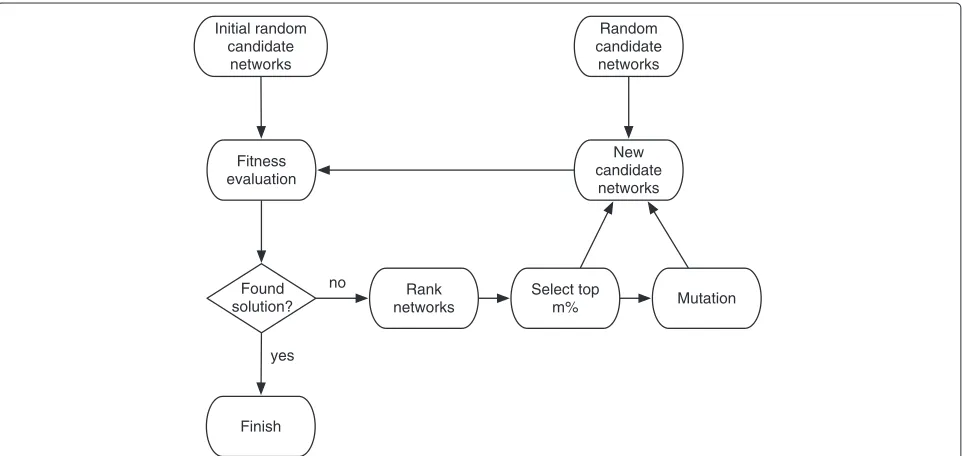
In this paper we explore the neutral space of the Schizosaccharomyces pombe(fission yeast) cell cycle regu-latory network. For this, we propose an evolutionary com-putation algorithm, in particular, an evolution strategy (ES), as a metaheuristic optimization algorithm that uses a mutation operator as its main search strategy (unlike GAs that use crossover and mutation) to generate a neutral graph of Boolean regulatory networks that share the same state sequences of the fission yeast cell cycle. We analyze the resulting neutral graph and compare characteristics of the regulatory networks that appear in the connected component of the original yeast cell cycle network with the networks that are not in the connected component, thus, given us a notion of the robustness of the model.

Results and discussion

Proposed evolution strategy (ES) for neutral graph construction

As mentioned in the background, a neutral graph is a metagraph (network of networks) where each node repre-sents a regulatory network that produces the same tem-poral evolution for a set of states out of the 2n possible configurations. In this paper, we considered the ten state sequences shown in Table 1. Following the terminology used in [14], regulatory networks that reproduce this tem-poral evolution will be calledfunctionalnetworks, while the original fission yeast cell cycle network will be called wildtypenetwork, which is a functional network as well given the previous definition. Although the wildtype net-work and a functional netnet-work will share the same state sequences of Table 1, they do not necessarily share the

dynamics produced by the remaining 210−10 states. The connectivity in a neutral graph is given by the Hamming distance of the interaction matrices (adjacency matrices) of the functional networks. Two nodes are connected if the Hamming distance of the respective functional net-work’s interaction matrices are equal to one, i.e., both matrices differ in only one element. The search in the neu-tral space for functional networks is huge, which makes it a difficult problem. The search consists in finding the weight matrix elementswijand the threshold vector

ele-mentsθithat can replicate the desired state sequences. To

carry out the search for functional networks, we propose an evolution strategy (ES) illustrated in the flow chart in Figure 1. Preliminary results using this technique appear in [23]. In what follows we will describe each stage.

Initial random candidate networks

A user defined parameter popSize indicates the size of the initial population. These are generated in the fol-lowing way. Using as a base the wildtype weight matrix and threshold vector, a new candidate network (solution) is obtained by changing ngh times the wildtype adja-cency matrix and threshold vector. The parameternghis selected randomly in the range of [1, 30], for every new candidate network generated. The wildtype weight matrix is changed using the following rule:

Rule 1

1. Select randomly a position(i,j)in the matrix.

2. If the position contains a non-zero number, then replace by a zero.

3. Else, replace with a value selected randomly from the

following set{−2,−1, 1, 2}.

The wildtype threshold vector is changed using the fol-lowing rule:

Rule 2

1. Select randomly a positioni in the vector.

2. Replace with a value selected randomly from the

following set{−2,−1,−1/2, 0, 1/2, 1, 2}.

both rules are repeatednghtimes.

Fitness evaluation

Each candidate network is evaluated in a fitness function defined as follows. The fitness function for the Boolean regulatory networkB, is computed by the deviation of the network’s output, defined byoi for each nodei, and the

target valuesi(sequence of the cell cycle) for each nodei:

fitness(B)= 1 10n

10

t=1

n

i=1

Table 1 Temporal evolution of sate vectors defining the fission yeast cell cycle

Time Start SK Cdc2/Cdc13 Ste9 Rum1 Slp1 Cdc2/Cd13* Wee1/Mik1 Cdc25 PP Phase

1 1 0 0 1 1 0 0 1 0 0 START

2 0 1 0 1 1 0 0 1 0 0 G1

3 0 0 0 0 0 0 0 1 0 0 G1/S

4 0 0 1 0 0 0 0 1 0 0 G2

5 0 0 1 0 0 0 0 0 1 0 G2

6 0 0 1 0 0 0 1 0 1 0 G2/M

7 0 0 1 0 0 1 1 0 1 0 G2/M

8 0 0 0 0 0 1 0 0 1 1 M

9 0 0 0 1 1 0 0 1 0 1 M

10 0 0 0 1 1 0 0 1 0 0 G1

wherenis the number of nodes in the network, and 10 is the number of state vector sequences (from Table 1) that the network must contain.

Rank networks

Given that the fitness function defines the deviation of the network’s output with respect to the desired target, the ES is formulated to solve a minimization problem, therefore, the candidate networks are ranked from the less deviated to the more deviated.

Select top m%

A user defined parameter mindicates the percentage of the ranked top solutions to be selected.

Mutation

Using the topm% solutions,(popSize−popSize×m%)/2 new candidate networks are generated using the following rule:

Rule 3

1. Select randomly one of the topm% solutions.

2. Mutate the selected solution. This is done by

applying Rule1 and Rule2 withngh=1.

this is repeated until completing the(popSize−popSize× m%)/2 new candidate networks.

Random candidate networks

To complete the popSize, the remaining (popSize − popSize×m%)/2 is filled with random candidate networks

Initial random candidate

networks

Found solution?

Random candidate networks

Fitness evaluation

Finish

Rank networks

Select top

m% Mutation

New candidate networks

yes no

generated using Rule1 and Rule2 withnghselected ran-domly in the range of [1, 30], for every new candidate network generated.

New candidate networks

The new population to be evaluated in the fitness func-tion, thus, completing the loop, is composed by the top m% solutions + the networks generates by the mutation stage + the networks generated randomly.

Simulations

The proposed ES was used to construct a neutral graph with functional networks that contain the fission yeast cell cycle state sequences of Table 1. In order to bound the search space, the elements of the weight matrices were constrained to the following integer values: {−2,−1, 0, 1, 2}, and the threshold vectors to:

{−2,−1,−1/2, 0, 1/2, 1, 2}. Also, popSize = 20, m% = 20% and max iterations =100.

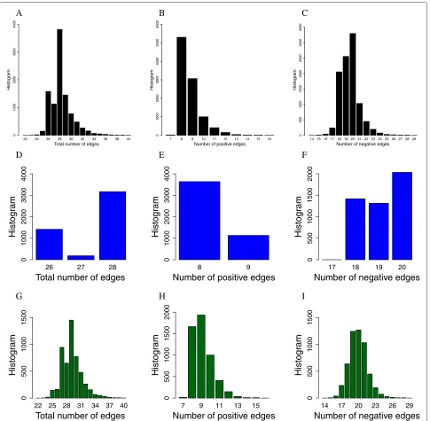
The ES was used to find 10000 functional networks. His-tograms of the resulting functional networks topologies are shown in Figure 2, where Figure 2A shows the distri-bution of the total number of edges (non-zero elements in the weight matrices) in the functional networks, Figure 2B shows the distribution of the number of positives edges and Figure 2C the distribution of the negative edges. If we consider that the wildtype network has a total of 27 edges composed of 8 positive edges and 19 negative edges, we can see from the histograms that in general the functional networks are mostly concentrated in these values but they can also have less or more edges then the wildtype.

The distribution of the edges changes if we separate the functional networks that belong to the wildtype con-nected component and the functional networks that are not in the connected component. Figure 2D,E and F are histograms from the wildtype connected component, showing that they are more concentrated around the wild-type topology whereas histograms G, H, and I are from functional networks that are not in the connected compo-nent, showing a larger dispersion.

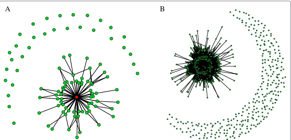
For visualization purposes we sampled 100 and 1000 functional networks from the 10000 found by the ES, to generate the neutral graph in Figure3A and Figure 3B respectively. The wildtype network appears in red (Color online). We notice that for functional networks not in the wildtype connected component, it is rare to see other con-nected components, in particular, in Figure 3B we see only one additional connected component besides the wild-type one, formed by two functional networks. From the wildtype connected component we notice that functional networks reach the wildtype in no more than 3 steps.

Biological robustness can be analyzed through the topological robustness of the functional networks in the wildtype connected component of the neutral graph. In

particular, one can identify which of the edges of these functional networks appear more frequent, and which are less frequent. This can give a notion of the regulatory rela-tions that are required, in a mandatory way in some cases, in order to complete the cell cycle sequence. For this sim-ulation, out of the 10000 functional networks, 330 are in the wildtype connected component. From these networks in the connected component, the positive edge that acti-vates the nodeSlp1 appears in 100% of the networks. This connection toSlp1 is necessary to ensure the integrity of the cell cycle, becauseslp1 mutant cells remain arrested in metaphase [24], therefore, the state sequences to com-plete the fission yeast cell cycle is interrupted in these cells. Another interesting case to point out are the double mutants rum1/wee1 andste9/wee1 which are not viable [25], therefore, all the networks in the wildtype connected component contain the positive edges that activatesSte9, Wee1 and Rum1, whereas, 0.6% of the non-connected component networks do not present the edge that acti-vatesSte9. In a similar way, 0.4% of the networks in the non-connected component do not present the edge that activatesWee1, and 0.5% do not present the edge that acti-vates Rum1. Surprisingly, by analyzing the networks in the wildtype connected component, only one connection appears out of the norm, in 43,9% of the networks, this is a positive edge fromSte9 toCdc25. This change in the topology of the wildtype network may allow the possibil-ity to formulate new biological hypotheses which could be tested.

22 24 26 28 30 32 34 36 38 40

Total number of edges

Histogr am 0 1000 2000 3000 4000 A

7 8 9 10 11 12 13 14 15 16

Number of positive edges

Histogr am 0 1000 2000 3000 4000 5000 6000 B

14 15 16 17 18 19 20 21 22 23 24 25 26 27 28 29

Number of negative edges

Histogr am 0 5 00 1000 1500 2000 2500 3000 3500 C

26 27 28

Total number of edges

Histogr am 0 1000 2000 3000 4000 D 8 9

Number of positive edges

Histogr am 0 1000 2000 3000 4000 E

17 18 19 20

Number of negative edges

Histogr am 0 500 1000 1500 2000 F

22 25 28 31 34 37 40

Total number of edges

Histogr a m 0 5 00 1000 1500 G

7 9 11 13 15

Number of positive edges

Histogr a m 0 500 1000 1500 2000 H

14 17 20 23 26 29

Number of negative edges

Histogr a m 0 5 00 1000 1500 I

Figure 2Histograms of the functional networks topologies of the neutral graph.ATotal number of edges;BPositive edges;CNegative edges;DTotal number of edges in the wildtype connected component;EPositive edges in the wildtype connected component;FNegative edges in the wildtype connected component;GTotal number of edges not in the wildtype connected component;HPositive edges not in the wildtype connected component;INegative edges not in the wildtype connected component.

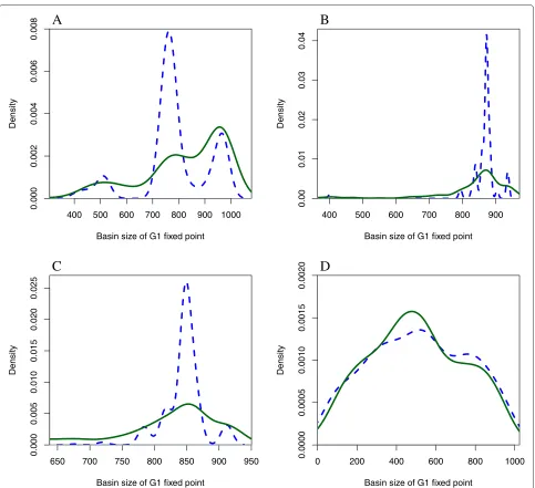
Figure 7 shows the state transition graph for the wildtype network using a sequential updating scheme. From these state transition graphs, one can appreciate the large basin of attraction for theG1fixed point.

Conclusions

An evolution strategy was developed to construct a neu-tral graph of Boolean regulatory networks that share the

A

B

Figure 3Neutral graph obtained using the proposed evolution strategy.(Color online) the red node represents the wildtype network. ANeutral graph using 100 functional networks;BNeutral graph using 1000 functional networks.

component of the wildtype network and the rest of the network, not only at a topological level, but also at the state space level, where significant differences in the dis-tribution of the basin of attraction for theG1fixed point was found for deterministic updating schemes, but not for the fully asynchronous updating scheme. From the results one can see that in general functional networks in the wildtype connected component, can mutate up to no more than 3 times, then they reach apoint of no return where the networks leave the connected component of the wildtype.

Finally, although the proposed evolution strategy was used for the fission yeast cell cycle model, it can be used to construct a neutral graph of other biological models under the Boolean network formalism. Moreover, the neutral space analysis of GRNs, may allow us to formulate new biological hypotheses studying the functional networks in the wildtype connected component, for example, analyz-ing which edges are in common, yieldanalyz-ing a core structure that could explain the preservation of the functionality of the network.

Methods Boolean networks

Letxbe a finite set ofnvariables,x = {x1,. . .,xn}, with

xi ∈ {0, 1}fori = 1,. . .,n. A Boolean network is a pair

(G,F), where G = (V,E) is a finite directed graph; V being the set ofn nodes and Ethe set of edges. F is a Boolean function,F : {0, 1}n → {0, 1}n composed of n

local functionsfi : {0, 1}n → {0, 1}. Furthermore, each

local functionfi depends only on variables belonging to

the neighborhood Vi = {j ∈ V|(j,i) ∈ E}. The

inde-gree of vertexiis|Vi|. The updating schemes are repeated

periodically, and since the hypercube is a finite set, the dynamics of the network converges to attractors which are fixed points or limit cycles, defined by

• Fixed point:xi(t+1)=xi(t)fori= {1,. . .,n}.

• Limit cycle:xi(t+p)=xi(t)fori= {1,. . .,n}.

wherep>1 is a positive integer called the period. The set of states that can lead the network to a specific attractor is called the basin of attraction. There are many ways of updating the values of a Boolean network, some examples are:

• Parallel or synchronous mode: where every node is

updated at the same time.

• Sequential updating mode: where in every time step,

every node is updated in a defined sequence.

• Block-sequential: the set of nodes, for a given

sequence, is partitioned into blocks. The nodes in a same block are updated in parallel, but blocks follow each other sequentially.

• Asynchronous deterministic: where in every time

step, one node is updated following a defined sequence.

• Fully asynchronous: where in every time step, one

400 500 600 700 800 900 1000

0.000

0.002

0.004

0.006

0.008

Basin size of G1 fixed point

Density

A

400 500 600 700 800 900

0.00

0.01

0.02

0.03

0.04

Basin size of G1 fixed point

Density

B

650 700 750 800 850 900 950

0.000

0.005

0.010

0.015

0.020

0.025

Basin size of G1 fixed point

Density

C

0 200 400 600 800 1000

0.0000

0.0005

0.0010

0.0015

0.0020

Basin size of G1 fixed point

Density

D

Figure 4Density of the basin of attraction for theG1fixed points of the functional networks in the wildtype component (blue/dashed line) and the rest of the networks (green/solid line).AUsing the parallel updating scheme;BUsing the following block sequential updating scheme (Start,SK,Cdc2/Cdc13)(Ste9,Rum1,Slp1,Cdc2/Cd13∗)(Wee1/Mik1,Cdc25,PP);CUsing the following sequential updating scheme (Start)(SK)(Cdc2/Cdc13)(Ste9)(Rum1)(Slp1)(Cdc2/Cd13∗)(Wee1/Mik1)(Cdc25)(PP);DUsing the fully asynchronous updating scheme.

An alternative to working with arbitrary logical gates in each node, is to consider a threshold Boolean network, where updates of each node are computed by

xi(t+1)=fi(x) = u ⎛ ⎝n

j=1

ωijxj(t)−θi ⎞

⎠ (2)

u(z) =

1, ifz≥0 0, ifz<0

with ωij the weight of the edge coming from node

j into the node i, and θi the activation threshold of

node i. The weights and thresholds are the network’s parameters.

Fission yeast cell cycle network

Figure 5Sate transition graph of the wildtype network using the parallel updating scheme.(Color online) The fix point states are represented by red circles and limit cycle states are represented by blue circles.

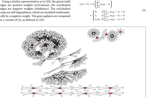
Using a similar representation as in [10], the green/solid edges are positive weights (activations), the red/dashed edges are negative weights (inhibitory). The red/dashed loops are self-degradation, which are modeled mathemati-cally by a negative weight. The gene updates are computed by a variant of (2), as defined in [10]:

xi(t+1)=u ⎛ ⎝n

j=1

wijxj−θi ⎞ ⎠

= ⎧ ⎪ ⎨ ⎪ ⎩

0, ifn_j=1wijxj−θi<0

1, ifn_j=1wijxj−θi>0 xi(t), ifn_j=1wijxj−θi=0

(3)

Figure 7Sate transition graph of the wildtype network using a sequential updating scheme.State transition graph using the following updating scheme (Start)(SK)(Cdc2/Cdc13)(Ste9)(Rum1)(Slp1)(Cdc2/Cd13∗)(Wee1/Mik1)(Cdc25)(PP). (Color online) the fix point states are represented by red circles.

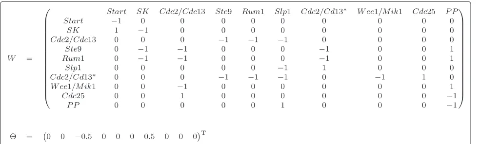
The weight matrix and the threshold vector used in (3) to generate the same dynamics exhibited in [10] appears in Figure 9. A complete dynamical study of this model can be found in [13].

In this model, three classes of molecules act: (1) The major role is played by a cyclin-dependent protein kinase

complex: Cdc2/Cdc13 with Tyr-15, a residue of Cdc2; (2) positive regulators of the kinase Cdc2/Cdc13: an indica-tor of the mass of the cell that works as “Start”, “Start kinase” (SK), a group of Cdk/cyclin complexes (Cdc2 with Cig1, Cig2 and Puc1 cyclins), and the phosphatase Cdc25; (3) antagonists of the complex Cdc2/Cdc13: Slp1, Rum1,

Cdc2/ Cd13* SK Start

Ste9

Cdc2/

Cd13 Rum1

Cdc25 PP

Slp1 Wee1

/Mik1

Figure 9Parameters for the fission yeast cell-cycle threshold Boolean network.Wrepresents the weight matrix andthe threshold vector.

Ste9, and the phosphatase PP. In theG1 phase, without the signal of cell size increase, the Cdc2/Cdc13 complex is inactive due to its antagonists. When the cell achieves a certain size, SK becomes active and a new round of cell division will begin by means of the accumulation of the Cdc2/Cdc13 complex. Cdc2/Cdc13 and SK dimers switch off the antagonists Rum1 and Ste9/APC in order to enter into the S phase. Moderate level on activity of the Cdc2/Cdc13 complex is enough for entering theG2 phase but not the mitosis, since proteins kinase Wee1 and Mik1 inhibits the activity of residue Tyr-15 of Cdc2. Then, to achieve theMphase, the activity of the Cdc2/Cdc13 complex must increase, and this occurs due to Cdc25 that reverses phosphorylation, removing the inhibiting phos-phate group and increasing the activity of the complex. High activity of the Cdc2/Cdc13 complex is represented in the network by a separate node called Cdc2/Cdc13*. An elevated activity level of Cdc2/Cdc13* at theMphase, activates Slp1/APC (Anaphase-Promoting complex). Slp1 degrades Cdc13, therefore, the Cdc2/Cdc13* complex is inhibited. At the end of theMphase the antagonists of Cdc2/Cdc13 are reset and the cell reaches theG1 station-ary state.

Using the parallel updating scheme, the cell cycle is modeled by starting from an initial state vector at time t = 1 and then the dynamics of the network produces sequences of state vectors untilt=10, where the network converges to a fixed point which represent theG1phase. Details of the previous sequences are shown in Table 1.

Competing interests

The authors declare that they have no competing interests.

Authors’ contributions

GAR and EG contributed in the design of the study. GAR proposed and implemented the evolution strategy, and run the simulations. GAR, TT, JB, and EG analyzed the results from the simulations. GAR and TT wrote the article. All the authors read and approved the final manuscript.

Acknowledgements

The authors would like to thank CONICYT-Chile under grant Fondecyt 11110088 (GAR), Fondecyt 1140090 (EG), CONICYT Doctoral scholarship (TT), and ANILLO ACT-88, for financially supporting this research.

Received: 6 June 2014 Accepted: 13 November 2014 Published: 25 November 2014

References

1. Akman OE, Watterson S, Parton A, Binns N, Millar A, Ghazal P:Digital clocks: simple Boolean models can quantitatively describe circadian systems.J R Soc Interface2012,9:2365–2382.

2. Li F, Long T, Lu Y, Ouyang Q, Tang C:The yeast cell-cycle network is robustly designed.PNAS2004,101:4781–4786.

3. Albert R, Othmer HG:The topology of the regulatory interactions predicts the expression pattern of the segment polarity genes in Drosophila melanogaster.J Theor Biol2003,223:1–18.

4. Mendoza L, Alvarez-Buylla ER:Dynamics of the genetic regulatory network for Arabidopsis thaliana flower morphogenesis.J Theor Biol

1998,193:307–319.

5. Espinosa-Soto C, Padilla-Longoria P, Alvarez-Buylla ER:A gene regulatory network model for cell-fate determination during Arabidopsis thaliana flower development that is robust and recovers experimental gene expression profiles.Plant Cell Online2004, 16:2923–2939.

6. Rangel C, Angus J, Ghahramani Z, Lioumi M, Sotheran E, Gaiba A, Wild D, Falciani F:Modeling T-cell activation using gene expression profiling and state-space models.Bioinformatics2004,20:1361–1372.

7. Fauré A, Naldi A, Chaouiya C, Thieffry D:Dynamical analysis of a generic Boolean model for the control of the mammalian cell cycle. Bioinformatics2006,22:e124–e131.

8. Bansal M, Della Gatta G, Di Bernardo D:Inference of gene regulatory networks and compound mode of action from time course gene expression profiles.Bioinformatics2006,22:815–822.

9. Kauffman SA:Metabolic stability and epigenesis in randomly constructed genetic nets.J Theor Biol1969,22:437–467.

10. Davidich MI, Bornholdt S:Boolean network model predicts cell cycle sequence of fission yeast.PLoS ONE2008,3(2):e1672.

11. Vera-Licona P, Jarrah A, Garcia-Puente LD, McGee J, Laubenbacher R: An algebra-based method for inferring gene regulatory networks. BMC Syst Biol2014,8(1):37.

12. Martin S, Zhang Z, Martino A, Faulon JL:Boolean dynamics of genetic regulatory networks inferred from microarray time series data. Bioinformatics2007,23(7):866–874.

13. Goles E, Montalva M, Ruz GA:Deconstruction and dynamical robustness of regulatory networks: application to the yeast cell cycle networks.Bull Math Biol2013,75:939–966.

15. Ciliberti S, Martin OC, Wagner A:Innovation and robustness in complex regulatory gene networks.PNAS1359,104:1–13596. 16. Ciliberti S, Martin OC, Wagner A:Robustness can evolve gradually in

complex regulatory gene networks with varying topology. PLoS Comput Biol2007,3:e15.

17. Holland JH:Adaptation in Natural and Artificial Systems. Ann Arbor, Michigan: University of Michigan Press; 1975.

18. Ruz GA, Goles E:Learning gene regulatory networks with predefined attractors for sequential updating schemes using simulated annealing.InProc. of IEEE the Ninth International Conference on Machine Learning and Applications (ICMLA 2010): IEEE; 2010:889–894.

19. Ruz GA, Goles E:Learning gene regulatory networks using the bees algorithm.Neural Comput Appl2013,22:63–70.

20. Ruz GA, Timmermann T, Goles E:Building synthetic networks of the budding yeast cell-cycle using swarm intelligence.InProceedings -2012 11th International Conference on Machine Learning and Applications, ICMLA 2012, Volume 1: IEEE; 2012:120–125.

21. Ruz GA, Goles E:Reconstruction and update robustness of the mammalian cell cycle network.In2012 IEEE Symposium on Computational Intelligence in Bioinformatics and Computational Biology (CIBCB 2012): IEEE; 2012:397–403.

22. Ruz GA, Goles E, Montalva M, Fogel GB:Dynamical and topological robustness of the mammalian cell cycle network: a reverse engineering approach.Biosystems2014,115:23–32.

23. Ruz GA, Goles E:Neutral graph of regulatory Boolean networks using evolutionary computation.InThe 2014 IEEE Conference on

Computational Intelligence in Bioinformatics and Computational Biology (CIBCB 2014): IEEE; 2014:1–8.

24. Kim SH, Lin DP, Matsumoto S, Kitazono A, Matsumoto T:Fission yeast Slp1: an effector of the Mad2-dependent spindle checkpoint.Science

1998,279(5353):1045–1047.

25. Sveiczer A, Csikasz-Nagy A, Gyorffy B, Tyson JJ, Novak B:Modeling the fission yeast cell cycle: Quantized cycle times in wee1−cdc25 mutant cells.Proc Natl Acad Sci2000,97(14):7865–7870.

doi:10.1186/0717-6287-47-64

Cite this article as:Ruzet al.:Neutral space analysis for a Boolean network model of the fission yeast cell cycle network.Biological Research201447:64.

Submit your next manuscript to BioMed Central and take full advantage of:

• Convenient online submission

• Thorough peer review

• No space constraints or color figure charges

• Immediate publication on acceptance

• Inclusion in PubMed, CAS, Scopus and Google Scholar

• Research which is freely available for redistribution