University of New Hampshire
University of New Hampshire Scholars' Repository
Master's Theses and Capstones
Student Scholarship
Spring 2019
Feature Selection by Singular Value
Decomposition for Reinforcement Learning
Bahram Behzadian
University of New Hampshire, Durham
Follow this and additional works at:
https://scholars.unh.edu/thesis
This Thesis is brought to you for free and open access by the Student Scholarship at University of New Hampshire Scholars' Repository. It has been accepted for inclusion in Master's Theses and Capstones by an authorized administrator of University of New Hampshire Scholars' Repository. For more information, please [email protected].
Recommended Citation
Behzadian, Bahram, "Feature Selection by Singular Value Decomposition for Reinforcement Learning" (2019).Master's Theses and Capstones. 1267.
Feature Selection by Singular Value Decomposition for Reinforcement Learning
BY
Bahram Behzadian
MASTER’S THESIS
Submitted to the University of New Hampshire in Partial Fulfillment of
the Requirements for the Degree of
Master of Science
in
Computer Science
ALL RIGHTS RESERVED
This thesis was examined and approved in partial fulfillment of the requirements for the degree of
Master of Science in Computer Science by:
Thesis Director, Marek Petrik, Assistant Professor
Department of Computer Science
Wheeler Ruml, Professor
Department of Computer Science
Laura Dietz, Assistant Professor
Department of Computer Science
Ernst Linder, Professor
Department of Mathematics and Statistics
On April 11, 2019
ACKNOWLEDGMENTS
I would like to thank my thesis advisor Marek Petrik of the Department of Computer Science at
the University of New Hampshire. Without his enthusiastic support and input, this work could not
TABLE OF CONTENTS
ACKNOWLEDGMENTS . . . iv
ABSTRACT . . . vii
Chapter 1 Introduction 1 1.1 Motivation . . . 2
1.2 Challenges and Contribution . . . 2
1.3 Outline . . . 4
Chapter 2 Linear Value Function Approximation 5 2.1 Components of Reinforcement Learning . . . 6
2.2 Mathematical Framework . . . 8
2.3 Value Function Approximation using Linear Architectures . . . 11
2.4 Policy Iteration and Approximate Policy Iteration . . . 17
Chapter 3 Feature Selection Methods 20 3.1 Proto-value Functions . . . 21
3.2 Diffusion Wavelets . . . 21
3.3 Eigenbasis of the Transition Matrix. . . 22
3.4 Krylov Subspace method. . . 24
3.5 Bellman Error Basis Function . . . 25
3.6 L1−regularized TD . . . 26
3.7 Approximate Linear Programming withL1 Regularization . . . 27
Chapter 4 FFS: Fast Feature Selection 29 4.1 FFS for Tabular Solution . . . 29
4.2 FFS for Approximate Solution . . . 31
Chapter 5 Empirical Evaluation 38
5.1 Synthetic Problems . . . 38
5.2 Cart-Pole . . . 42
Chapter 6 Conclusion, Discussion and Future Directions 47
6.1 Future Work . . . 47
6.2 Conclusion . . . 47
ABSTRACT
Feature Selection by Singular Value Decomposition
for Reinforcement Learning
by
Bahram Behzadian
University of New Hampshire, May, 2019
Solving reinforcement learning problems using value function approximation requires having good
state features, but constructing them manually is often difficult or impossible. We propose Fast
Feature Selection (FFS), a new method for automatically constructing good features in problems
with high-dimensional state spaces but low-rank dynamics. Such problems are common when,
for example, controlling simple dynamic systems using direct visual observations with states
repre-sented by raw images. FFS relies on domain samples and singular value decomposition to construct
features that can be used to approximate the optimal value function well. Compared with earlier
methods, such as LFD, FFS is simpler and enjoys better theoretical performance guarantees. Our
experimental results show that our approach is also more stable, computes better solutions, and
CHAPTER 1
Introduction
Reinforcement Learning (RL) involves the problem of automatic decision making from experience
(Sutton & Barto, 2018). As an agent travels through the state space, it needs to identify and
nav-igate to states with higher rewards. By definition, a value function measures the expected rewards
attainable from each state and makes it possible to pick good actions quickly. While value functions
can be computed efficiently in small Markov decision processes, computing them in problems with
(infinitely) many states is challenging (Puterman, 2014).
Most RL approaches for solving problems with large state spaces rely on some form of value function
approximation (Sutton & Barto, 2018; Szepesv´ari, 2010). Linear Value Function Approximation
(VFA) is one of the most frequent and most straightforward approximation methods. It represents
the value function as a linear combination of state features. Each feature should represent some
essential characteristics of the state space. As with linear regression, it is necessary to use only
features that are relevant. Using too many features can cause overfitting and prohibitive
computa-tional complexity.
Linear methods are interpretable (easy to understand), easy to implement, and easy to analyze in
comparison to black box methods such as artificial neural networks (Lagoudakis & Parr, 2003).
Significant effort has been devoted to automating feature construction for linear VFA. Examples
of methods that construct features—or select them from a large set—include proto-value
func-tions (Mahadevan & Maggioni, 2007), diffusion wavelets (Mahadevan & Maggioni, 2006), Krylov
TD (Kolter & Ng, 2009), and`1-regularized approximate linear programming (Petrik, Taylor, Parr,
& Zilberstein, 2010).
1.1
Motivation
Although linear value function approximation is less powerful than modern deep reinforcement
learning, it is still important in many domains. In particular, linear models are interpretable and
need relatively few samples to compute a value function reliably. Features also make it possible
to encode prior knowledge conveniently. Finally, the last layer in deep neural networks, used for
reinforcement learning, often calculates a linear combination of the underlying neural network
fea-tures (Song, Parr, Liao, & Carin, 2016).
Our goal is to compute a small set of useful features from the transition matrix and the reward
function. However, such parameters are practically unavailable. Therefore we are compelled to
esti-mate the transition matrix and reward function from samples. Using singular value decomposition
over such estimation guarantees that the extracted features are linearly independent (Lagoudakis
& Parr, 2003).
1.2
Challenges and Contribution
Recently researchers worked on value function approximation (VFA) problems with high
dimen-sional state space both with deep neural nets (Mnih, Kavukcuoglu, Silver, Graves, Antonoglou,
Wierstra, & Riedmiller, 2013; Mnih, Badia, Mirza, Graves, Lillicrap, Harley, Silver, & Kavukcuoglu,
2016; Oh, Guo, Lee, Lewis, & Singh, 2015) and linear architectures (Song et al., 2016). In this
thesis, we propose Fast Feature Selection (FFS), a new feature selection method that uses Singular
Value Decomposition (SVD) to compute a low-rank approximation of the transition matrix and
As with all data-driven methods, feature construction (or selection) must make some simplifying
assumptions about the problem structure, which can be used to reduce the number of samples
needed. We assume the matrix of transition probabilities can be closely approximated using a
low-rank matrix. Using the low-rank approximation has led to significant successes in several machine
learning domains, including collaborative filtering (Murphy, 2012), natural language word
embed-dings (Li, Zhu, & Miao, 2015), reinforcement learning (Ong, 2015; Cheng, Asamov, & Powell,
2018), and Markov chains (Rendle, Freudenthaler, & Schmidt-Thieme, 2010). Surprisingly, given
the simplicity and popularity of SVD in other areas of machine learning, it has not been previously
used for feature compression in reinforcement learning. Our theoretical analysis also leads to new
approximation error bounds that translate the singular values of the transition matrix to the
ap-proximation error.
A significant limitation of linear value function approximation is that it requires good features
to approximate the optimal value function well. This is difficult to achieve since good a priori
estimates of the optimal value functions are rarely available. Considerable effort has, therefore,
been dedicated to methods that can automatically construct useful features or at least select
them from a larger set. Examples of such methods include proto-value functions (Mahadevan
& Maggioni, 2007), diffusion wavelets (Mahadevan & Maggioni, 2006), Krylov bases (Petrik, 2007),
BEBF (Parr, Painter-Wakefield, Li, & Littman, 2007), L1−regularized TD (Kolter & Ng, 2009), and L1-regularized ALP (Petrik et al., 2010), and supervised sparse coding (Le, Kumaraswamy, &
White, 2017).
This work focuses on batch reinforcement learning (Lange, Gabel, & Riedmiller, 2012). In batch
RL, all domain samples are provided in advance as a batch, and it is impossible or difficult to
gather additional samples. This is common in many practical domains. In medical applications,
applications, it may take an entire growing season to obtain a new batch of samples.
Another assumption that we make is that there are many raw state features available. For example,
in video games, raw features can be derived directly from the pictorial representation of the game.
Because the raw features are too numerous, using them directly would lead to prohibitive sample
complexity. Our goal is to compute a small set of useful features as a linear combination of raw
features.
FFS is easy to implement, and our experiments show that it is faster, more robust, and results in
a lower Bellman error compared to similar methods. We also establish new theoretical guarantees
on the Bellman error as a function of the spectrum of transition matrices.
1.3
Outline
The remainder of the thesis proceeds as follows. Chapter 2 summarizes the framework of linear
value function approximation and the relevant Markov decision process properties. In Chapter 3,
we review common feature selection and construction methods. Chapter4 describes our new Fast
Feature Selection method (FFS) and analyzes its approximation error and then compares it with
other feature construction algorithms. Finally, the empirical evaluation in Chapter5indicates that
FFS is faster and more robust than competing methods. We discuss future work and conclude this
CHAPTER 2
Linear Value Function Approximation
In reinforcement learning (RL) we are interested in automatic decision making under uncertainty
using the history of the agent. This decision-making problem can be formulated in an Markov
Decision process (MDP) framework. Such environments are assumed to be fully observable. The
current state is Markovian (memoryless) and completely characterizes the state of process. In this
chapter, we briefly introduce reinforcement learning problems and their components. Then we
explain the principle of MDPs and describe some dynamic programming methods that solve them.
Finally, we discuss the concept of value function approximation and linear approximation methods.
Reinforcement learning is different from supervised learning since no supervision determines the
right or wrong behavior. An RL agent only relies on a reward signal from the environment. Such
feedbacks are delayed and not instantaneous so the result of a good action cannot be recognized
immediately. Time plays a vital role in RL because the agent is processing data sequentially, which
means the training dataset is neither independent nor identically distributed (Sutton & Barto,
2018). Most importantly, any action taken by an agent may influence the environment and change
the subsequent data it receives.
A reward signal rt is a feedback from the environment as a scalar real number that indicates how
well the agent is performing at each time step t. In reinforcement learning, the agent’s goal is
defined by a hypothesis that all goals can be represented by the maximization of the expected
cumulative reward (Sutton & Barto, 2018). Therefore, an RL agent has to behave in a certain way
2.1
Components of Reinforcement Learning
In this section, we describe the essential components of RL and explain their relationships. We
introduce the mathematical framework for MDPs, which is the critical element in solving a
rein-forcement learning problem.
2.1.1 Agent and Environment
In RL problems, an agent is the brain of the system, which, in each time step t, makes a decision
and executes an actionat. Meanwhile, it receives an observation otand a scalar rewardrtfrom the
environment. We can describe the environment as everything else in the world. At each time step
t, the environment receives an actionatfrom the agent and emits an observationot+1 and a scalar
rewardrt+1. The time increments in discrete steps.
2.1.2 History and State
All observations, rewards, and actions from the first time step until the current time tare referred
to as the history and are denoted withHt={a1, o1, r1, . . . , at−1, ot, rt}. What happens in the future
depends on the history and the agent’s actions. The environment determines the observations and
rewards. A state is the information used to determine what happens next. The state is a sufficient
statistic of the history and can be formally written as a function of historySt=f(Ht) (Sutton &
Barto, 2018).
A state can be regarded from three different points of view. From the environment point of view,
the state Ste is whatever data the environment uses to pick the next observation and reward. The
that even if visible to the agent, they do not help for a better decision making.
From the agent’s internal representation, the stateSat is whatever information the agent uses to pick
the next action. An agent’s state contains the information that is used by reinforcement learning
algorithms and can be any function of history.
Finally, the information stateStalso known as Markov state which represents the useful information
from the history. A state is Markovian if and only if P[St+1|St] = P[St+1|S1, . . . , St]. In another
word, the future is independent of the past given the present information stateSt. Therefore, once
we have the current state, we can throw away the history and rely on the current state for the
future decision making. It is important to note that the environment state and the history are
Markov state as well.
2.1.3 Agent’s Components
The major components of an RL agent may include one or more of the following:
• Model: It describes the agent’s representation of the environment. A model predicts what the environment might do next. A model predicts the next state with a transition matrixP
and next immediate reward R given the current state St=s.
• Policy: Agent behavior is expressed as a functionπ known as policy that maps any observed state to an action or a probability distribution over actions. When the policy is deterministic
the return of policy for each state is a single action a=π(s). A randomized policy return a
probability distribution over actions: P[At=a|St=s] =π(a|s).
• Value Function: It maps any state or action to a real number. The value of a state somehow predicts the expected cumulative future rewards that could be achieved from that particular
state onwards. The state values are used to evaluate the goodness or badness of being in each
2.2
Mathematical Framework
Markov decision processes (MDPs) formally describe an environment for reinforcement learning,
where the environment is fully observable. An environment is fully observable when the agent
di-rectly observes the environment state in a way thatot=Sta=Ste. Almost all RL problems can be
described as MDPs. For example, optimal control primarily deals with continuous MDPs. Partially
observable Markov decision process problems can be converted to MDPs. Bandits are MDPs with
a single state.
All states in MDPs are Markov states, which means the future is independent of the past given
the present state, and the state holds all necessary information in the history. In this section, we
start with explaining the Markov process environments, and we will continue with Markov reward
process and Markov decision process.
2.2.1 Markov Process
A Markov process (a.k.a Markov chain) is a memoryless random process with a sequence of states
(S1, S2, . . .) with the Markov property. Such processes can be defined as a tuple hS, Pi, where S is a finite set of Markov states and P is the state transition probability matrix. So we have
pss0 =P[St+1=s0|St=s].
2.2.2 Markov Reward Process
A Markov reward process (MRP) is a Markov process (S1, R2, S2, . . .) with rewards for each state.
MRP is a tuplehS, P, R, γi. S and P are defined exactly like a Markov process, but R:S →Ris
a reward function and can be shown asrs=E[Rt+1|St=s]. The discount factorγ ∈[0,1] controls
the agents preference over short-term rewards and long-term rewards. The return Gt is the total
Gt=Rt+1+γRt+2+γ2Rt+3+. . .= ∞
X
k=0
γkRt+k+1
When γ is close to zero, we say the agent is myopic or short-sighted and prefers to collect rewards
as fast as possible. On the other hand, whenγ is close to one, we say the agent is far-sighted and
tries to collect maximum cumulative rewards possible even though it may take much more time
than a short-sighted agent. The discount factor adjusts the value of the rewards in future for the
following reasons (Sutton & Barto, 2018; Puterman, 2014):
• It is mathematically convenient to discount the future rewards since we can estimate a bounded return for every state.
• To avoid infinite reward loops in cyclic Markov processes.
• The model may not account for uncertainty in the future very well, so it is less likely to gain future rewards compare to immediate rewards.
As outlined earlier, the value functionv(s) represents the long-term value of each states. In MRPs,
the state value function is the expected return starting from any states.
v(s) =E[Gt|St=s].
The value function can be decomposed into two parts: The immediate reward Rt+1 and the
dis-counted value of successor state γv(St+1). The Bellman equation for MRPs is base on this idea of
decomposition of the value function (Puterman, 2014). Indeed, the value function must satisfy:
v(s) =E[Rt+1+γv(St+1)|St=s] = (2.1)
=rs+γ
X
s0∈S
pss0v(s0) . (2.2)
The Bellman equation can also be stated using matrices as follows:
where v is a column vector with one entry per state1. Since (2.3) is a linear equation, we can
solve it directly with v = (I−γP)−1r. However, the best achieved computational complexity of inverting a matrix isO(n2.37) (Coppersmith & Winograd, 1990), so the closed form solution is not
efficient for large state spaces. There exist many iterative solutions for large MRPs such as dynamic
programming and Monte-Carlo evaluation (Sutton & Barto, 2018).
2.2.3 Markov Decision Process
A Markov decision process (MDP) is a Markov reward process with decisions. It is an environment
in which all states are Markov. An MDP is a tuple hS,A, P, R, γi in which A is a finite set of actions. The transition probability and reward function also depend on action taken from each
state:
pass0 =P[St+1=s0|St=s, At=a] (2.4)
ras =E[Rt+1|St=s, At=a] (2.5)
The solution to an MDP is a policy. A policyπ is a distribution over actions conditioned on states
π(a|s) =P[At=a|St=s]. A policy in MDPs fully defines the behavior of an agent and it depends
only on the current state instead of the full history. Every Markov decision process with a policy
π can be converted to a Markov process hS, Pπi if we only sample the state sequence (S1, S2, . . .) that follows the policy π. The same rule applies for an MRP hS, Pπ, Rπ, γi when we only sample the state and reward sequence (S1, R2, S2, R3, . . .) where:
pπs,s0 =
X
a∈A
π(a|s)pass0 (2.6)
rsπ =X
a∈A
π(a|s)rass0 (2.7)
In an MDP environment, value function can be defined as state-value function vπ(s) and
action-value funcion qπ(s, a). The state-value function of an MDP is the expected return starting from
1
state s, and then following policy π, vπ(s) =Eπ[Gt|St =s]. The action-value function qπ(s, a) = Eπ[Gt|St=s, At=a].
Bellman Equation
Both state-value function and the action-value function can be decomposed into immediate reward
and discounted value of the next state (Sutton & Barto, 2018):
vπ(s) =Eπ[Rt+1+γvπ(St+1)|St=s] (2.8)
qπ(s, a) =Eπ[Rt+1+γqπ(St+1, At+1)|St=s, At=a]. (2.9)
We can express Bellman expectation equation in a concise form using induced MRP with vπ =
rπ+γPπvπ, therefore the direct solution would bevπ = (I−γPπ)−1rπ.
Bellman Optimality Equation
The objective of an MDP is to find an optimal policy,π∗, such that vπ∗(s) =v∗(s)≥vπ(s) for all
s∈ S and for all policies Π. The optimal state-value functionv∗(s) is the maximum value function over all policies:
v∗(s) = max
π v
π(s).
The optimal action-value functionq∗(s, a) is the maximum action-value function over all policies.
q∗(s, a) = max
π q
π(s, a).
An MDP is considered solved when we know the optimal value function.
2.3
Value Function Approximation using Linear Architectures
A value function in contexts RL maps every state to a real number that represents the value of
where the number of states is not so large, we can store the value of each state in a table; the
agent can look it up while traversing the environment. Such representation of value function is also
known as the tabular representation of the value function.
With a large state space, we cannot rely on tabular solution methods since the number of states
can be so large that makes storing the value function as a table impossible. The difficulty with
large state spaces is not only the memory storage but also the generalization (Sutton & Barto,
2018). Generalization concerns with how the experience of a subset of data can be generalized to
a much larger state space. In RL, the generalization can be made using function approximation.
With function approximation, we can collect samples for a subset of states and then generalize
from them to build an approximation of the entire function.
Although with function approximation, we can generalize the state space, it is hard to manage,
control, and understand. Some problems may arise with function approximation such as:
• Non-stationarity: learning a value function based on a subset of the data is useful only if we assume that the dynamics of the environment remain stationary. In other words, an
optimal learned policy remains optimal if the parameters of the environment such as transition
probabilities and reward function remain unchanging. However, generalization might fail if
the world’s parameters are non-stationary (Da Silva, Basso, Bazzan, & Engel, 2006).
• Dynamic learning: Neural nets and statistical learning approaches all assume a static training set over which many passes are made. In RL, learning is performed by collecting data via
interaction with environments so learning a value function requires to be able to deal with
incrementally acquired data (Bertsekas & Tsitsiklis, 1996).
• Bootstrapping: Semi-gradient (a.k.a bootstrapping) approaches do not converge as robustly as gradient methods, but they work reliably in the linear case (Sutton & Barto, 2018).
recent activity of the agent. Therefore, the difference between good and bad actions might
remain undetected if we rely on limited samples.
In reinforcement learning, function approximation techniques are applied to estimate the value
func-tion. The idea is to approximate a value function from simulated data from a known policy. This
value function is represented by parameters that we learn through sampling from experience and it
is usually denoted as ˆvπ(s,w) or in the case of state-action value function we have ˆqπ = (s, a;w).
In a linear function approximation, the vector w ∈ Rk represent the features’ weights. If we
ap-proximate the value function using a multilayer artificial neural network, w stands for the vector
of connection of layers. Typically, the number of parameterskis smaller than the number of states
S, so each parameter corresponds to many more states at the same time. Whenever a single state is updated, it affects many other states. Therefore, value function approximation theory raises the
idea of generalization in learning and make approximation methods more powerful but harder to
understand (Sutton & Barto, 2018). In RL systems it is necessary to consider that learning occurs
while interacting with the environment, so the agent should be able to learn from incrementally
collected data. The agent also needs to account for functions that can handle non-stationary target
function.
Function approximation methods are applied where the value function cannot be computed
pre-cisely. Most Markov Decision Process (MDP) in real-world have continuous or high-dimensional
state spaces, which demand function approximation to work efficiently. These methods reduce the
state space of the problem to a lower dimension. In the following section, we describe one of the
linear methods, which are the most common approach for value function approximation and are
easy to analyze theoretically.
2.3.1 Linear Value Function Approximation
In this section, we summarize the background on linear value function approximation. Value
can then be approximated by a linear combination of features φ1, . . . , φk∈R|S|, which are vectors
over states. Using the vector notation, an approximate value function ˆvπ can be expressed as:
ˆ
vπ = Φw,
for some vectorwof scalar weights that quantify the importance of features. It is well-known that
the value functionvπ for a policyπ must satisfy the Bellman optimality condition (e.g., (Puterman,
2014)):
vπ =rπ+γPπvπ , (2.10)
wherePπ andrπ are the matrix of transition probabilities and the vector of rewards, respectively,
for the policy π. The feature matrix Φ is of dimensions |S| ×k; (k |S|) the columns of this matrix are the featuresφi. Φ ={φ1, . . . , φk}in this equation is a set of linearly independent basis
functions of the state. The weights vector w = {w1, . . . , wk} is a set of scalars that need to be
estimated through the process of approximation. The vectorwquantify the importance of features.
Here, Φ is the feature matrix of dimensions|S| ×k; the columns of this matrix are the features φi.
Because of its simplicity and interpretability, linear function approximation techniques are one of
the most common techniques for RL.
One of the advantages of basis functions is mitigating the curse of dimensionality of these practical
problems (Keller, Mannor, & Precup, 2006). The produced basis functions Φ still describe the high
dimensional state space but with some information loss. Numerous algorithms such as linear TD(λ),
LSTD, and LSPE for computing linear value function approximation have been proposed (Sutton
& Barto, 2018; Lagoudakis & Parr, 2003; Szepesv´ari, 2010). We focus on fixed-point methods that
compute the unique vector of weightswπΦ that satisfy the projected Bellman equation (2.10):
wπΦ= Φ+(rπ+γPπΦwπΦ) , (2.11)
where Φ+ denotes the Moore-Penrose pseudo-inverse of Φ (e.g., Golub and Van Loan (2013)). This
(2.10).
In order to construct good features, it is essential to be able to determine their quality in terms
of whether they can express a good approximate value function. The standard bound on the
performance loss of a policy computed using, for example, approximate policy iteration can be
bounded as a function of the Bellman error (e.g., Williams and Baird (1993)). To motivate FFS,
we use the following result that shows that the Bellman error can be decomposed into the error in
1) the compressed rewards, and in 2) the compressed transition probabilities.
Theorem 1 ((Song et al., 2016)). Given a policy π and features Φ, the Bellman error of a value
functionv= ΦwΦπ satisfies:
BEΦ= (rπ−ΦrπΦ)
| {z }
∆π r
+γ(PπΦ−ΦPΦπ)
| {z }
∆π P
wπΦ .
We seek to construct a basis that minimizes both k∆π
rk2 and k∆πPk2. These terms can be used to bound the L2 norm of Bellman error as:
kBEΦk2 ≤ k∆πrk2+γk∆πPk2kwΦπk2≤ ≤ k∆πrk2+γk∆PπkFkwπΦk2 ,
(2.12)
where the second inequality follows from kXk2≤ kXkF.
The Bellman error (BE) decomposition in (2.12) has two main limitations. The first limitation is
that it is expressed in terms of the L2 norm rather than L∞ norm, which is needed for standard
Bellman residual bounds (Williams & Baird, 1993). This can be addressed, in part, by using the
weighted L2 norm bounds (Munos, 2007). The second limitation of (2.12) is that it depends on
kwπΦk2 besides the termsk∆π
rk2,k∆πPk2 that we focus on. Sincekw
π
2.3.2 Linear Models Approximation
In the linear model approximation, we aim to approximate the transition model using linearly
in-dependent features Φ. Such features are required to approximate next state feature values Φ(s0|s) and reward function rgiven the current state. The idea is similar to linear value function
approx-imation approach. Parr et al. (2008) shows that the same set of features that predict a reliable
value function can be implemented for approximating the linear model.
Given a basis function Φ = {φ1, . . . , φk} for a linear value function or a linear model, a feature
vector Φ(s) = [φ1(s), . . . , φk(s)]> can be defined withφi(s) representing value of feature iin state
s. Meanwhile, Φ(s0|s) is defined as the random vector of next features (Parr et al., 2008):
Φ(s0|s) = [φ1(s0), . . . , φk(s0)]> , (2.13)
where s0 ∼P(s0|s). The idea is to generate a matrix PΦ ∈ Rk×k that predicts the expected next
feature vector:
PΦ>Φ(s)≈Es0∼P(s0|s){Φ(s0|s)} (2.14)
And minimizes the expected feature prediction error:
PΦ = arg min
Pk
X
s
P
>
k Φ(s)−E{Φ(s0|s)}
2
2 (2.15)
One way to solve this optimization problem is to find the least-squares solution to the system
ΦPΦ ≈PΦ. Given the policyπ, the solution to the system would be:
We can also implement a standard least-squares projection into span(Φ) to compute an approximate
reward predictor:
rπΦ= (Φ>Φ)−1Φ>rπ = Φ+rπ . (2.17)
with corresponding approximate reward ˆr= ΦrπΦ.
2.4
Policy Iteration and Approximate Policy Iteration
Policy iteration (Howard, 1960) also known as actor-critic architectures (Barto, Sutton, & Anderson,
1983; Sutton & Barto, 1984) is a process of identifying the optimal policy for any given MDP. Policy
iteration is an iterative method in the space of deterministic policies; it finds the optimal policy by
performing a series of monotonically improving policies. Every iteration consists of two stages:
• Stage one: policy evaluation (also recognized as the critic) calculates the state-action value function of given policy. Policy evaluation solves the linear system of the Bellman equations.
• Stage two: policy improvement (which is also recognized as the actor) describes the improved greedy policy. The resulting policy is a deterministic policy which is at least as good as the
previous policy.
These two stages are repeated until the calculated policy is the same as the previous one. In this
phase, we claim that the iteration has converged to the optimal policy. We can guarantee the
convergence of policy iteration to the optimal policy only in the event of a tabular representation of
the value function (exact solution), and tabular representation of policy (Lagoudakis & Parr, 2003).
Such precise representations and approaches are unrealistic for large state and action spaces.
There-fore, approximation methods are applied to mitigate the curse of dimensionality. Approximations
in the policy-iteration structure can be presented at two points:
• In the policy representation: The tabular representation of the policy is substituted by a parametric representation ˆπ(s;θ)
In each case, merely the parameters of the representation must be saved, and we require a much
smaller memory to store the parameters than the tabular case. The critical factor for a good
approximate algorithm is the determination of the parametric approximation structure and the
decision of the projection method (Lagoudakis & Parr, 2003).
2.4.1 Least-Squares Temporal Difference (LSTD)
LSTD is a temporal difference algorithm based on the theory of linear least-squares function
approx-imation, and it is introduced by Bradtke and Barto (1996). The idea is that a linear architecture
approximates the state value function and its representation Φ is consist of a compact description
of the essential functions and a set of parameters wΦ:
wΦ= (I−γ(Φ>Φ)−1Φ>PΦ)−1(Φ>Φ)−1Φ>r (2.18) = (Φ>Φ−γΦ>PΦ)−1Φ>r . (2.19)
LSTD is sample-efficient and converges quicker than TD(λ) (Sutton, 1988). LSTD is useful for
prediction problems when the agent is learning the value function of a fixed policy. It does not
have any use in control problems because LSTD learns the state-value function of a fixed policy
and can not be applied in action selection without learning a model of the underlying MDP.
2.4.2 Least-Squares Policy Iteration
It is not practical to use LSTD directly as policy evaluation for a policy iteration algorithm. Koller
and Parr (2000) present an instance of LSTD-style function approximation and policy iteration
where the policy changes between two poor performances in an MDP with a small number of
states. Least-Squares Policy Iteration (LSPI) suggested by Lagoudakis and Parr (2003) is a
to control problems. LSPI mixes the policy-search effectiveness of policy iteration with the data
efficiency of LSTDQ.
For instance, in the LSPI algorithm, the linear approximation for state-action value function
(q-function) is adopted from LSTD and extended to LSTDQ, which performs the weighting of the
features. However, LSTDQ approximates q-functions applying a different feature set for each
pos-sible action.
LSPI learns the state-action value function which allows for action selection without a model. It
is sample-efficient, off-policy algorithm that reuses samples in each iteration. Besides, it does not
require any parameter tuning since learning parameters, such as the learning rate, are omitted.
In the following chapter, we review the most relevant techniques for feature selection which have
CHAPTER 3
Feature Selection Methods
In the previous chapter, we discussed Least-Squares Policy Iteration (LSPI) for linear Value
Func-tion ApproximaFunc-tion (VFA) which employs previously chosen sets of features. LSPI tends to evaluate
the approximated function, analyze the features, tweaking them, and re-running the approximator
until the approximation is consistent. This approach by itself is not satisfying, as this iterative
process of trying different feature sets until success depends on human intuition, dismantling the
concept of autonomous artificial intelligent agents. Feature selection methods attempt to automate
this process in a way that maintain the low computational cost of linear approximation (Petrik
et al., 2010).
A significant limitation of linear value function approximation is that it requires good features,
which is, features that can represent the state space properly and be able approximate the optimal
value function well. This is often a difficult goal to achieve since good priori estimates of the
optimal value functions are rarely available. Considerable effort has therefore been dedicated to
methods that can automatically construct useful features for linear value function approximation.
Examples of methods that construct features, or select good features from a large set, include
proto-value functions (Mahadevan, 2005), diffusion wavelets (Mahadevan & Maggioni, 2006), Fourier
Basis (Konidaris, Osentoski, & Thomas, 2011), Krylov bases (Petrik, 2007), BEBF (Parr et al.,
2007), L1−regularized TD (Kolter & Ng, 2009), and approximate linear programs (Petrik et al., 2010). In this chapter, we briefly describe some of the most common methods in feature selection
3.1
Proto-value Functions
Mahadevan (2005) introduced Proto-Value Functions (PVFs), which is a specific instantiation of
a general scheme for basis functions by diagonalizing symmetric diffusion operators. PVFs are
created by employing the eigenvectors of the graph Laplacian on an undirected graph (N, E) is
made of state transitions to develop a basis for linear value function approximation.
The states of the MDP express nodes of an undirected weighted graph given a fixed policy. This
graph can be defined by a symmetric adjacency matrix W, where each element of the matrix
de-notes the weight between the nodes. A diagonal matrix D of the node degrees is determined as
Dxx =Py∈NWxy. The benefit of the normalized Laplacian is that it is symmetric, and therefore
its eigenvectors are orthogonal (Petrik, 2007). Proto-value functions presenting a compressed
rep-resentation of the powers of transition matrices and they span the entire space of possible value
functions for a given state space.
3.2
Diffusion Wavelets
Mahadevan and Maggioni (2006) introduce two methods for automatically constructing basis
func-tions on state spaces that can be represented as graphs or manifolds. The first way is to use the
eigenfunctions of the Laplacian similar to Proto-value functions; another approach is based on
dif-fusion wavelets, which generalize classical wavelets to graphs.
The extension of the Laplacian approach with Diffusion Wavelet Transforms (DWT) is a
com-pact multi-level representation of Markov diffusion processes on manifolds and graphs. Diffusion
wavelets are used to perform a fast multi scale analysis of functions on a manifold or graph, which
are generalizing wavelet analysis and associated with signal processing techniques such as
The diffusion wavelets create a low-order approximation of the inverse of a matrix. One of the
disadvantages of applying the wavelets for VFA is the massive computational cost required to build
the inverse approximation. However, once the inverse is constructed, it can be reused for different
rewards as long as the transition matrix is fixed (Petrik, 2007).
3.3
Eigenbasis of the Transition Matrix
Eigenvalues of a square matrix A ∈ Rn×n play an important role in dynamic problems such as
du/dt=Au. Almost all vectorsx∈Rnwill have a new direction after multiplication byA. There
are some exceptions which are known as eigenvectors. Eigenvectors x stay in the same direction
after such multiplication by A. The result ofAxis a vector λtimes the originalxso we can write
Ax=λx. The number λis an eigenvalue ofA. The eigenvalue λcan tell whether the eigenvector
is expanded or shrunk or reversed or remains unchanged (Strang, 2009). To compute eigenvalues
we need to set the determinant of A−λI to zero. Solving det(A−λI) = 0 result in eigenvalues, however to find the eigenvectors we need to find all vectors in the Null-space of A−λI. For each eigenvectorλ, any vectorxthat is a solution for (A−λI)x= 0 is an eigenvector for A.
The matrix A can be transformed to a diagonal matrix Λ when we use the eigenvectors properly.
Suppose A is a n by n matrix with n linear eigenvectors x1, . . . ,xn. We can put all eigenvector
into the columns of an eigenvector matrix S.
A matrixAcan be diagonalized asS−1AS = Λ where Λ is a diagonal matrix filled with eigenvalues
of A. This form of matrix factorization is called diagonalization, and can be shown in different
forms as well:
AS =SΛ or A=SΛS−1 (3.1)
The matrix S is invertible because we assumed the eigenvectors of A to be linearly independent.
Without independent eigenvector, diagonalization is impossible. Also, some matrices do not have
contain repeated eigenvalue can be diagonalized. It worth mentioning that invertibility and
diag-onalizability are two different issues. A matrix is invertible when no eigenvalue is equal to zero
(λ 6= 0). However, diagonalizability is only concerned with the available eigenvectors. Enough independent eigenvector from differentλsatisfies diagonalizability.
Difference-equation is an equation that recursively represents a sequence. Once the primary terms
are given, any further term of the sequence is determined as a function of the previous terms. A
typical difference-equation isuk+1=Auk. At each step, the current state ukmultiplies byA. The
solution for such difference equation is uk =Aku0. Diagonalization of matrix A provides a quick
way to calculate Ak. Assume S is the matrix of eigenvectors of A. According to equation (3.1)
matrix A can be written asA =SΛS−1. This form of factorization is suitable for computing the
powers of A. The reason is that every time S−1 multiplies S we getI:
Aku0 = (SΛS−1)· · ·(SΛS−1)u0=SΛkS−1u0 (3.2)
We can splitSΛkS−1u
0 as follows. First, we can write u0 as a combination of eigenvectorsc1x1+ · · ·+cnxn. Then c = S−1u0. Then we need to multiply each eigenvector xi by λki so we have
ΛkS−1u0. And finally we add up the ciλkixi to get the solution uk = Aku0. The solution for
uk+1 =Auk would be:
uk=Aku0=c1λk1x1+· · ·+cnλknxn (3.3)
If A is a Markov matrix, all entries ofA are positive, and all rows sum up to 1. These properties
guarantee that the largest eigenvalue of A is λ = 1 (Strang, 2009). Considering that P is the
transition matrix (Markov matrix) for a fixed Markov policy, we can represent the value function
as (Puterman, 2014):
v= (I−γP)−1r= ∞
X
i=0
(γP)ir. (3.4)
Let assume the transition matrix is diagonalizable and x1, . . . ,xn are n linearly independent
vector as a mixture of eigenvectors similar tou0 in the deference equation problem.
r=c1x1+· · ·+cnxn= n
X
j=1
cjxj (3.5)
Forc=S−1r, and usingPixj =λijxj we have (Petrik, 2007):
v= n X j=1 ∞ X i=1
(γλj)icjxj = n
X
j=1 1 1−γλj
cjxj = n
X
j=1
djxj (3.6)
Considering a subsetU of eigenvectors xj as a basis for linear value functionv the error bound on
the approximation would be:
kv−vˆk2 ≤X
j /∈U
|dj|. (3.7)
The value function can be approximated by using thatxj’s with greatest |dj|.
3.4
Krylov Subspace method
Alexei Krylov, a Russian applied mathematician introduce the concept of Krylov subspace in 1931.
Krylov subspace Kn(A,b) is the subspace spanned by b, Ab, . . . , An−1b. Petrik (2007) proposed a
value function approximation based on Krylov subspaces, and denoted these vectors as yi = Pir
for i∈ [0, n−1]. The Krylov basis constructs a basis that minimizes the Bellman error kv−vˆk in each iteration. The major issue with Krylov vectors is that they are far from orthogonal.
The Arnoldi iteration creates an orthonormal basis q1, q2, . . . for the same space using the
Gram-Schmidt technique. Arnoldi iteration orthogonalize each new vector against the previous one (see
algorithm1). The Krylov subspace spanned byr, Pr, . . . , Pn−1r then will have much better basis
Algorithm 1:Arnoldi Iteration
Input: Transition matrixP, rewardsr, and number of features k
1 q1 =r/krk ;
2 for n= 1 to k−1 do 3 v=P qn ;
4 forj= 1 to ndo
5 hjn=qj>v ;
6 v=v−hjnqj ;
7 end
8 hn+1,n=kvk; 9 qn+1 =v/hn+1,n ;
10 end
11 return Approximation features: Φ ={q1, . . . ,qk}.
3.5
Bellman Error Basis Function
Bellman Error Basis Function (BEBF) is a well-known method for expanding already given
ba-sis functions for linear value function (Parr et al., 2007). The idea behind BEBF is taken from
Bellman-error-based methods (Keller et al., 2006) in which the new feature φk+1 is obtained from
bellman error of approximated value function with already calculated set of features Φ∈R|S|×k.
Let ˆv = Φw be the approximated value function. We can obtain φk+1 =Tvˆ−vˆ where T is the Bellman operator. φk+1 is orthogonal to the span of Φ and is a Bellman Error Basis Function
(BEBF) for constructing a new design matrix Φ0 = [Φ, φk+1] when we concatenate the column
vector to the previews set of features. The Bellman error is an intuitively interesting approach to
3.6
L
1−
regularized TD
The Least-Squares Temporal Difference (LSTD) algorithms (see section 2.4.1) are employed for
learning the parameters of the linear value function. The naive implementation of LSTD only uses
the trajectories generated by the simulator. However, when the number of features is enormous,
LSTD can overfit to data and become computationally expensive. Kolter and Ng (2009) propose an
L1-regularization method that provides sparse solutions and behaves as a feature selection process.
Given nsamples of (s, a, r, s0) from system trajectories we can formn×k feature matrices Φ and Φ0 and the reward vector r. LSTD computes the fixed point of the following equation:
w= ˆf(w) = arg min
u∈Rk
Φu−(r+γΦ0w)
2
D (3.8)
The solution follows analytically by solving the linear system:
w= (Φ>(Φ−γΦ0))−1Φ>r=A−1b (3.9)
To limit overfitting, particularly when the number of samples are smaller than the number of
features (m < k), Kolter and Ng (2009) add a regularization penalty function to the equation (3.8).
w= ˆf(w) = arg min
u∈Rk 1 2
Φu−(r+γΦ0w)
2
D +βkuk1 (3.10)
Because the equation (3.10) is not convex and non-differentiable, the optimal solution w can be
constructed incrementally. it is desirable to apply an algorithm known as Least Angle Regression
(LARS) (Efron, Hastie, Johnstone, Tibshirani, et al., 2004) and updating one element of w at a
time until we approach the exact solution of the optimization problem. BecauseL1regularization is
known to provide sparse solutions, it can provide for more efficient implementation and be beneficial
3.7
Approximate Linear Programming with
L
1Regularization
For large MDPs, one way to approximate value function is employing Approximate Linear
Pro-gramming (ALP) (Schweitzer & Seidmann, 1985; de Farias & Van Roy, 2005). Given a set of
features Φ and a linear space M ⊆ R|S|, where M = span{Φ} and its first column is 1 we can formulate the problem as the following optimization problem:
min v∈M
X
s∈S
ρ(s)v(s)
subject to r(s, a) +γX
s0∈S
P(s, a, s0)v(s0)≤v(s)
(3.11)
where ρ is the distribution over the initial states. For the sake of simplicity, one can reformulate
the optimization problem in (3.11) by using an ALP constraint matrix L. The constraint matrix has the property of Lv ≤ v that is equivalent to the set {Lav ≤ v : ∀a ∈ A}. La denotes the
Bellman update.
min
v ρ
>v
subject to Lv≤v
v ∈ M
(3.12)
As we mentioned in the previous section, the approximate dynamic programming approach requires
a small set of appropriate features to find a reliable solution. However, when the number of features
is enormous, the solution may cause to over-fit when the number of samples is limited. ALP
approach is not an exception. Petrik et al. (2010) suggest an L1 regularization technique for
approximate linear programming (RALP) to overcome such problems. L1 regularization can pick
number of selected features. The RALP for basis Φ andL1 constraint ψ is defined as follow:
min
v ρ
>Φw
subject to LΦw≤Φw
kwk1,e ≤ψ ,
(3.13)
where kwk1,e is the weighted L1 norm for the value function parameters. RALP with sampled constraints guarantees that the solution is bounded and also presents worst-case error bounds on
the value function (Petrik et al., 2010).
In the next chapter, we introduce a new feature construction algorithm that can extract a basis for
CHAPTER 4
FFS: Fast Feature Selection
In this chapter, we describe the proposed method for selecting features from a low-rank
approxi-mation of the transition probabilities. To simplify the exposition, we first introduce the method
for the tabular case and then extend it to the batch RL setting with many raw features in section4.2.
4.1
FFS for Tabular Solution
Algorithm 2:TFFS: Tabular Fast low-rank Feature Selection
Input: Transition matrixP, rewards r, and number of featuresk
1 Compute SVD decomposition of P: P =UΣV> ;
2 Assuming decreasing singular values in Σ, select the first k−1 columns ofU:
U1←[u1, . . . ,uk−1] ;
3 return Approximation features: Φ = [U1,r].
The Tabular Fast Feature Selection algorithm is summarized in Algorithm 2. Informally, the
algorithm selects the top k−1 singular vectors and the reward function for the features. Our error bounds show that including the reward function as one of the features is critical. It is not
surprising that when the matrix P is of a rank at most k then using the first k singular vectors
will result in no approximation error. However, such low-rank matrices are rare in practice. We
now show that it is sufficient that the transition matrix P is close to a low-rank matrix for TFFS
P be SVD(P) =UΣV>, where
U =
U1 U2
, Σ =
Σ1 0
0 Σ2
, V =
V1 V2
.
That implies that the transition probability matrix can be expressed as:
P =U1Σ1V1>+U2Σ2V2> .
Let matrixU1havekcolumns and let the singular values be ordered decreasingly. Then, algorithm2
generates Φ =U1. The following theorem bounds the error regarding the largest singular value for
a vector not included in the features.
Theorem 2. Assuming k features Φ computed by Algorithm 2, the error terms in 1 are upper
bounded as:
k∆Pk2 ≤ kΣ2k2,
k∆rk2 = 0 .
Proof. From the definition of ∆P and PΦ we get the following equality:
∆P =UΣV>U1−U1(U1>U1)−1U1>UΣV>U1 .
Recall that singular vectors are orthonormal which implies that (U1>U1)−1=IandU1>U =
I1 0
.
Substituting these terms into the equality above, we get:
k∆Pk2 =
(UΣV
>−U1Σ1V>
1 )U1
2 ≤ UΣV
>−U
1Σ1V1>
2kU1k2 .
Simple algebraic manipulation shows that UΣV>−U1Σ1V1>
2 = kΣ2k2 and kU1k2 = 1 because U is an unitary matrix. This establishes the inequality for ∆P; the result for ∆r follows directly
from the properties of orthogonal projection sincer itself is included in the features.
Theorem2 implies that if we choose Φ in a way that the singular values in Σ2 are zero (when the
no approximation error becausek∆Pk2 = 0. More broadly, when the rank of the matrix is greater than k, the error is minimized by choosing the singular vectors with the greatest singular values.
That means that TFFS chooses features Φ that minimize the error bound in Theorem 2.
4.1.1 Contributions
In this section, we present TFFS, an exact solution algorithm for fast low-rank feature selection.
Theorem2provides an upper error bound on Bellman error for the TFFS’s approximation features.
4.2
FFS for Approximate Solution
Using TFFS in batch RL is impractical since the transition matrix and reward vector are usually
too large and are not available directly. The values must instead be estimated from samples and
the raw features.
Algorithm 3:FFS: Fast low-rank Feature Selection from raw features
Input: Sampled raw featuresA, next state of raw featureA0 , rewardsr, and number of
featuresk
1 Estimate compressed transition probabilities PA=A+A0 as in LSTD ;
2 Compute SVD decomposition of PA: PA=UΣV> ;
3 Compute compressed reward vector: rA=A+r ;
4 Assuming decreasing singular values in Σ, select the first k−1 columns ofU:
U1←[u1, . . . ,uk−1] ;
5 return Approximation features: Φ = [b U1,rA].
As described in the introduction, we assume that the domain samples include a potentially large
compressed transition matrix is denoted as PA = A+P A and compressed rewards are denoted as
rA=A+rand are computed as in equations (2.16) and (2.17). To emphasize that the matrixP is
not available, we use A0 =P A to denote the expected value of features after one step. Using this
notation, the compressed transition probabilities can be expressed asPA=A+A0.
Algorithm 3 describes the FFS method that uses raw features. Similarly to TFFS, the algorithm
computes an SVD of the transition matrix. Note that the featuresΦ are linear combinations of theb
raw features. To get the actual state features, it is sufficient to computeAΦ whereb Φ is the outputb
of Algorithm3. The matrixΦ represents features forb PA and is of a dimensionl×kwhere lis the
number of raw features inA. We omit the details for how the values are estimated from samples,
as this is well known, and refer the interested reader to Lagoudakis and Parr (2003) and Johns,
Petrik, and Mahadevan (2009).
Using raw features to compress transition probabilities and rewards is simple and practical, but
it is also essential to understand the consequences of relying on these raw features. Because FFS
computes features that are a linear combination of the raw features, they cannot express more
complex value functions. FFS thus introduces additional error—akin to bias—but reduces sampling
error—akin to variance. The following theorem shows that the errors due to our approximation
and using raw features merely add up with no additional interactions.
Theorem 3. Assume that the raw featuresAforP and computed featuresΦb forPAare normalized,
such that kAk2 =
Φb
2 = 1. Then:
k∆AΦb
P k2 ≤ k∆
A
Pk2+k∆
b
Φ
PAk2 , k∆AΦb
r k2 ≤ k∆
A
rk2+k∆
b
Φ
rAk2 ,
where the superscript of∆indicates the feature matrix for which the error is computed; for example
∆Φb
PA =PAΦb −Φ(b PA)Φb .
∆,
∆
AΦb P 2 =
P AΦb−AΦbPAΦb
2 .
Now, by adding a zero (APAΦb−APAΦ) and applying the triangle inequality, we get:b
∆
AΦb P 2 =
P AΦb−APAΦ +b APAΦb−AΦbPAΦb
2 ≤ ≤
P AΦb−APAΦb 2+
APAΦb−AΦbPAΦb
2 .
Given (AΦ)b +=Φb+A+ and the property of the compressed transition matrix in equation (2.16) we
can show:
(PA)Φb −PAΦb =Φb
+P
AΦb−(AΦ)b +P AΦb
=Φb+(PA−A+P A)Φ = 0b
∆
AΦb P
2
≤ kP A−APAk2
Φb 2+ +
PAΦb−Φ(b PA)Φb
2kAk2 .
The theorem then follows directly from algebraic manipulation and the fact that the features are
normalized.
Note that the normalization of features required in Theorem 3can be achieved by multiplying all
features by an appropriate constant, which is an operation that does not affect the approximate
value function. Scaling features does, however, affect the magnitude of wΦ, which, as we discuss
above, is problem-specific and largely independent of the feature selection method used.
Perhaps one of the most attractive attributes of FFS is its simplicity and low computational
com-plexity. Selecting the essential features only requires computing the singular value decomposition—
for which many efficient methods exist—and augmenting the result with the reward function. As
We described FFS in terms of singular value decomposition and showed that when the
(com-pressed) transition probability matrix has a low rank, the approximation error is likely to be small.
Next, we describe the relationship between FFS and other feature selection methods in more detail.
4.2.1 Contributions
In this section, we introduce a fast low-rank feature selection algorithm that uses raw feature
inputs to generate approximation features for linear value function. We also show in Theorem 3
that using raw features and feature approximation simultaneously does not result in additional
interaction error.
4.3
Related Feature Selection Methods
In this section, we describe similarities and differences between FFS and related feature
construc-tion or selecconstruc-tion methods.
Perhaps the best-known method for feature construction is the technique of proto-value
func-tions (Mahadevan & Maggioni, 2006, 2007). Proto-value functions are closely related to spectral
approximations (Petrik, 2007). This approximation uses the eigenvector decomposition of the
tran-sition matrixP =SΛS−1, whereS is a matrix with eigenvectors as its columns and Λ is a diagonal
matrix with eigenvalues that are sorted from the largest to the smallest. The first kcolumns of S
are then used as the approximation features. As with our FFS method, it is beneficial to augment
these features with the reward vector. We will refer to this method as EIG+R in the numerical
re-sults. Surprisingly, unlike with FFS, using the topk eigenvectors does not guarantee zero Bellman
residual even if the rank of P is less than k.
referred to as BEBF (Parr et al., 2007, 2008). The Krylov subspace Kis spanned by the images of
r under the firstkpowers of P (starting fromP0 =I):
Kk(P,r) = span{r, Pr, . . . , Pk−1r}.
Petrik (2007) shows that whenkis equal to the degree of the minimal polynomial, the approximation
error is zero. Krylov methods are more likely to work in different problem settings than either
EIG+R or FFS and can be easily combined with them.
Algorithm 4:LFD: Linear Feature Discovery for a fixed policy π (Song et al. 2016).
1 D0 ←random(k, l); 2 i←1;
3 while Not Converged do
4 Ei←A+A0Di−1 ;
5 Di ←(AEi)+A0; 6 i←i+ 1 ; 7 end
8 return Ek // Same role as Φb in FFS.
Finally, Linear Feature Discovery (LFD) (Song et al., 2016) is a recent feature selection method
that is closely related to FFS. Algorithm4depicts a simplified version of the LFD algorithm, which
does not consider the reward vector and approximates the value function instead of the q-function
for a fixed policyπ. Recall that A is the matrix of raw features andA0 =Pπ.
LFD is motivated by the theory of predictive optimal feature encoding. A low-rank encoder Eπ is
predictively optimal if there exist decodersDπs and Dπr such that:
AEπDsπ =PπA , AEπDrπ =rπ .
2016). Unfortunately, it is almost impossible to find problems in practice in which a predictively
op-timal controller exists. No bounds on the Bellman error are known when a controller is merely close
to predictively optimal. This is in contrast with the bounds in Theorems2and3that hold for FFS.
Although LFD appears to be quite different from FFS, our numerical experiments show that it
computes solutions that are similar to the solutions of FFS. We argue that LFD can be interpreted
as a coordinate descent method for computing the following low-rank approximation problem:
min
E∈Rl×k,D∈Rk×l
kAED−A0k2F . (4.1)
This is because the iterative updates of Ei and Di in Algorithm 4 are identical to solving the
following optimization problems:
Ei ←arg min
E∈Rl×kkAEDi−1−A
0k2
F
Di ←arg min
D∈Rk×lkAEiD−A
0k2
F
The equivalence follows directly from the orthogonal projection representation of linear regression.
This kind of coordinate descent is a very common heuristic for computing low-rank matrix
com-pletions (Hastie, Mazumder, Lee, & Zadeh, 2015). Unfortunately, the optimization problem in
equation (4.1) isnon-convex and coordinate descent, like LFD, may only converge to a local
opti-mum, if at all. Simple algebraic manipulation reveals that any set ofk singular vectors represents
a local minimum of LFD. Finally, we are not aware of any method that can solve equation (4.1)
optimally.
Similarly to LFD, FFS solves the following optimization problem:
min
E∈Rl×k,D∈
Rk×l
kED−A+A0k2F . (4.2)
This fact follows readily from the SVD decomposition of A+A0 and the fact that the Frobenius
norm is equal to the L2 norm of the the singular values (Hastie, Tibshirani, & Friedman, 2009;
Note that when the using tabular features (A = I) the optimization problems in equation (4.1)
and equation (4.2) are identical. For any other raw features, there are two reasons for preferring
equation (4.2) over equation (4.1). First, FFS is much easier to solve both in theory and in practice.
Second, as Theorem3shows, the approximation error of FFS is simply additive to the error inherent
to the raw features. No such property is known for LFD. In the next chapter, we compare the two
CHAPTER 5
Empirical Evaluation
In this section, we empirically evaluate the quality of features generated by FFS both with and
without using raw features. We focus on a comparison with LFD (Song et al., 2016) which was
empirically shown to outperform radial basis functions (RBFs) (Lagoudakis & Parr, 2003), random
projections (Ghavamzadeh, Lazaric, Maillard, & Munos, 2010), and other methods.
We first compare the quality of solutions on a range of synthetic randomly-generated problems. The
goal is to ensure that the methods behave similarly regardless of the number of samples, or the type
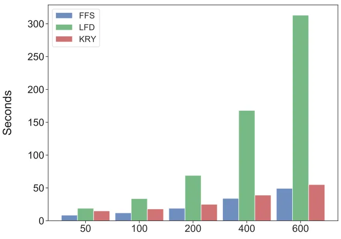
of raw features that are used. Then, we use an image-based version of the cart-pole benchmark,
used previously by Song et al. (2016), to evaluate FFS in more complex settings. This problem is
used to evaluate both the solution quality and the computational complexity of the methods.
5.1
Synthetic Problems
To compare FFS to other common approaches in feature selection, we start with small policy
evaluation problems. Since the policy is fixed throughout these experiments, we omit all references
to it. The data matrix A ∈ Rn×l only contains the states where n denotes the number of states
and lthe length of each raw feature, with Φ∈Rn×k using kfeatures.
The synthetic problems that we use throughout this section have 100 states. The rewards r ∈
R100 are generated uniformly randomly from the interval of [−500,500). The stochastic transition
probabilities P ∈ [0,1)100×100 are generated from the uniform Dirichlet distribution. To ensure that the rank of P is at most 40, we compute P as a product P = XY, where X and Y are
0 20 40 60 80
Number of Features used for VFA
10−10
10−8
10−6
10−4
10−2
100
102
B
E
=
ΔR
+
γ
ΔP
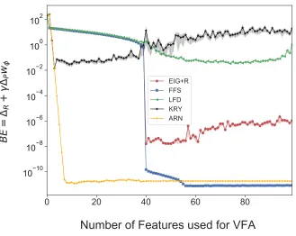
wϕ
EIG+R FFS LFD KRY ARN
Figure 5-1: Bellman error for the exact solution. The transition matrix is 100×100 and has a low rank with rank(P) = 40. The Input matrix isA=I an identity matrix.
We now proceed by evaluating FFS for both tabular and image-based features. For the sake of
consistency, we use FFS to refer to both FFS in a tabular case and FFS when raw features are
available. To evaluate the quality of the value function approximation, we compute the Bellman
residual of the fixed-point value function, which is a standard metric used for this purpose. Recall
that the Bellman error can be expressed as
BE = ∆r+γ∆PwΦ,
where wΦ is the value-function given in equation (2.18). All results we report in this section are
an average of 100 repetitions of the experiments. All error plots show theL2 norm of the Bellman
error in logarithmic scale.
Case 1: Tabular raw features. In this case, the true transition probabilities P and the
re-ward function r are known, and the raw features are an identity matrix: A = I. Therefore all
This is the simplest setting, under which SVD simply reduces to a direct low-rank approximation
of the transition probabilities. That is, the SVD optimization problem reduces to:
min
U1∈Rn×k
min Σ1V1>∈Rk×n
kU1Σ1V1>−Pk2F .
Similarly, the constructed features will be Φ =U1. In case of TFFS, we can simply add the reward
vector to feature’s set Φ = [U1,r]. EIG+R and KRY are implemented as described in (Petrik, 2007;
Parr et al., 2008). In case of EIG+R approach, we use the eigenvectors of P as basis functions,
and thenr is included. For Krylov basis we calculate Φ =Kk(P,r). We also include the result of Arnoldi iteration (ARN) using Algorithm1.
Figure 5-1 depicts the Bellman error for the exact solution when the number of features used for
value function varies from 1 to 100. Note that the Bellman error of FFS is zero fork≥40. This is because the rank ofP is 40, and according to Theorem2the first 40 features obtained by FFS are
sufficient to getkBEk2= 0. This experiment shows FFS is robust and generally outperforms other methods. The only exception is the Krylov method which is more effective when few features are
used but is not numerically stable with more features. However, Arnoldi iteration does not suffer
from this problem. The Krylov method could be combined relatively easily with FFS to get the
best of both bases.
Case 2: Image-based raw features. In this case, the raw features A are not tabular but
instead simulate an image representation of states. So the Markov dynamics are experienced only
via samples and the functions are represented using an approximation scheme. The matrix A is
created by randomly allocated zeros and ones similar to the structure of a binary image. We use
LSTD to compute the approximate value function, as described in section2.3.1.
The SVD optimization problem now changes as described in section 4.2. The constructed features
will be Φ =AΦ and for FFS we include the reward predictor vector [b PA,rA] in the optimization
problem. In the case of the EIG+R method, we multiply the eigenvectors of PA and rA with the
raw features. The Krylov basis is constructed as: Φ = AKk(PA,rA) where Kk is the k-th order