REDUCTION USING SEMI CORRELATION FACTOR

(1)

REDUCTION USING

SEMI CORRELATION FACTOR

A. A. Abo Khadra

Department of Physics and Engineering Mathematics, Faculty of Engineering, Tanta University, 31521,Tanta, Egypt.

Department of Mathematics, Faculty of Science, Tanta University, Tanta, Egypt.

Department of Physics and Engineering Mathematics, Faculty of Engineering, Kafrelsheikh University, 33516, Kafrelsheikh, Egypt.

E-mail: [email protected]

Abstract:

In this paper, we need to define a new definition for a correlation factor using semi rough sets technique. This definition is very simpler than statistic definition, that gives us a capability to deal with all information tables (quantities and qualitative). By using this definition, the boundary region will be decreased according to the increasing of the positive and negative regions. We can make the reduction of any information system tables by using the definition of semi correlation factor.

Keywords: rough set, rough set correlation factor, semi rough set correlation factor, reduction.

1. Introduction

Rough set theory (RST) was proposed by Zdzislaw Pawlak in 1982. Since then we have witnessed systematic, world-wide growth of interest in rough set theory and its applications. The theory of rough sets deals with the classificatory analysis of data tables. The data can be acquired from measurements or from human experts. The main purpose of the rough set analysis is the induction of approximations of concepts from the acquired data. The classical rough set analysis is based on the indiscernibility relation that describes indistinguishability of objects. The concepts are represented by their lower and upper approximations. In applications, rough sets focus on approximate representing of knowledge derivable from data. It leads to significant results in the areas including, e.g., data mining, machine learning, finance, industry, multimedia, medicine, control theory, pattern recognition, and most recently bioinformatics [3,5-16].

In this paper we recall some basic notions related to rough sets and the extension of RST via correlation factor .Also, we mention some measures of closeness of concepts and measures comprising entire decision systems .Finally, we propose some new measures for reduction of information systems.

The approach we used depends on the positive region between the condition attribute and decision attribute or classified attributes "attributes which make a classification of objects as classes ". The positive region gives us a new definition of correlation factor which valid for all data "quantities, qualitative, ordered and unordered data". This definition is very simpler than statistic definition [2] that gives us a capability to deal with all information tables.

2. Basics Rough Set Concepts

(2)

called decision table).



a



A

there is a corresponding function

f

_a

:

U



V

_a, where

V

_a is the set of values of a. If

P



A

, there is an associated equivalence relation:

)}

(

)

(

,

|

)

,

{(

)

(

P

x

y

U

a

P

f

x

f

y

IND











_a



_a (1)

The partition of U, generated by IND (P) is denoted U/P. If

(

x

,

y

)



IND

(

P

)

, then x and y are indiscernible by attributes from P. The equivalence classes of the P-indiscernibility relation are denoted

[

x

]

_P. Let

X



U

, the P-lower approximation

P

X

and P-upper approximation

P

X

of set X can be defined as:

}

]

[

|

{

x

U

x

X

P





_P



(2)

}

]

[

|

{











x

U

x

X

P

_P (3)

Let

P

,

Q



A

be equivalence relations over U, then the positive, negative and boundary regions can be defined as:

X

P

Q

POS

Q U X

P

(

)



_



_/ (4)

X

P

U

Q

NEG

Q U X P

(

)





_



_/

(5)

X

P

X

P

Q

BND

Q U X Q U X

P

(

)



_



_/



_



_/

(6)

The positive region of the partition U/Q with respect to P,

POS

_P

(

Q

)

, is the set of all objects of U that can be certainly classified to blocks of the partition U/Q by means of P. Q depends on P in a degree k (

0 

k



1

) denoted

P



_k

Q

U

Q

POS

Q

k





_P

(

)



P

(

)

(7)

If k=1, Q depends totally on P, if 0<k<1, Q depends partially on P, and if k=0 then Q does not depend on P. When P is a set of condition attributes and Q is the decision,



_P

(

Q

)

is the quality of classification [10]. The goal of attribute reduction is to remove redundant attributes so that the reduced set provides the same quality of classification as the original. The set of all reducts is defined as:

)}

(

)

(

,

),

(

)

(

|

{

Red



R



C



_R

D





_C

D



B



R



_B

D





_C

D

(8)

A dataset may have many attribute reducts. The set of all optimal reducts is:

}

,

Red

|

Red

{

Red

_min



R





R





R



R



(9)

3. Rough Set Correlation Factor

(3)

upper approximation as interior and closure operators from topology [4] instead of using the indiscernibility relation of rough set.

Definition 1.

Let U be an universe and A={C,D} be a set of condition attributes C and decision attribute D, [1] then

||

({ }, ) ||

,

||

,

1, 2,3,....,| |

i i

i

POS

c

D

r

U

c

C i

C







(10)

be a correlation factor

r

_ibetween attribute ci and decision attribute D.

4. Semi Rough Set Correlation Factor

We will introduce a new definition for semi correlation factor by using semi rough set technique. This definition will decrease the boundary region by increasing the positive and negative regions.

Definition 2.

Let (U, R) be a general knowledge base [1] R

R.

Let X  U, for each x



U, R(x) = {y: x R y} will be called a neighborhood of x. The topology  generated by the subbase SR={R(x): x



U} is not generally Pawlak

topology, it coincides with it if R is an equivalence relation.

A class SR is called a subbase for the topology



on U iff finite intersection of members of SR form a base

R

 of



.

A class _R is called a base for topology



if each of member of



is the union of members of _R.

Definition 3.

Let (U, R) be a general knowledge base R

R.

Let X  U, the general lower and upper approximation of X in U denoted



(X) and  (X) are defined as follows [1,3]:



X = {G: G



 and G  X} ₍₁₁₎

 X = {F: F



c_{and F}__X}

(12)

Definition 4.

Let U be an universe and A={C,D} be a set of condition attributes C and decision attribute D, then

|| _ ({ }, ) || , || ||

, 1, 2,3,....,| |

i S i

i

S POS c D

r

U

c C i C



 

where

(13)

/ ( )

S_ POS(C,D) =

SY

Y U IND D

(4)

S

Y = Y  (



(Y)) (15)

S i

r

is a semi correlation factor between attribute ci and decision attribute D.

S_ POS(C,D)

is a semi positive

region.

S

Y is a semi lower approximation of a set Y.

5. Reduction Using Semi Correlation Factor

Data reduction is an important step in knowledge discovery from data [14,15]. The high dimensionality of databases can be reduced using suitable techniques, depending on the requirements of the data mining processes. These techniques fall in to one of two categories: those that transform the underlying meaning of the data features and those that are semantics-preserving. Feature selection (FS) methods belong to the latter category, where a smaller set of the original features is chosen based on a subset evaluation function.

The process aims to determine a minimal feature subset from a problem domain while retaining a suitably high accuracy in representing the original features. In knowledge discovery, feature selection methods are particularly desirable as these facilitate the interpretability of the resulting knowledge.

Rough set theory has been used as such a tool with much success, enabling the discovery of data dependencies and the reduction of the number of features contained in a dataset using the data alone, requiring no additional information.

In this paper; by using semi correlation factor we can make a reduction of information system tables as follows:

Let C



A, a



C,

If

r

_{S a}



1

, then Red={a}, and if

If

r

_{S a}



0

, then Red=A-{a}

If

If 0



r

_{S a}



1

, then we can remove attribute a with some approximation depending on the value of

r

_{S a}

If

r

_{S C}



1

, then Red=B, and if

If

r

_{S C}



0

, then Red=A-C

If

If 0



r

_{S C}



1

, then we can remove attributes C with some approximation depending on the value of

r

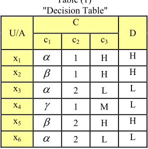
_{S C} See the following examples.

Example 1.

Let U={x1,x2,x3,x4,x5,x6} be an universe, A={C,D} be an attributes, C={c1,c2,c3} be condition attributes, some

of its values are unordered values as



,



,



,H,L and M; others are ordered values as 1,2; and D be a decision attribute as shown in the following table:

Table (1) "Decision Table"

U/A C D

c1 c2 c3

x1



1 H H

x2



1 H H

x3



2 L L

x4



1 M L

x5



2 H H

x6



2 L L

Using semi rough set technique, we get; Sub-base of topology Sc1 is:

(5)

Base of topology βc1 is

βc1={Ф,{ x1,x3,x6},{x2,x5},{x4}}

Then the topology τ c1 is:

τ c1={U,Ф,{ x1,x3,x6},{x2,x5},{x4},{ x1, x2, x3, x5,x6},{ x1,x3, x4,x6},

{ x2, x4, x5}}. And the complement of topology  c1 is:

τ c1c = c1={Ф,U,{ x2, x4, x5},{ x1,x3, x4,x6},{ x1, x2, x3, x5,x6},{ x4},

{ x2,x5},{x1,x3,x6}} U/IND({D}={{x1,x2,x5},{x3,x4 ,x6}}

Y1={x1,x2,x5} Y2={{x3,x4,x6}

S

Y1= Y1 (



(Y1))={x2,x5},

S

Y2= Y2 (



(Y2))={x4}

1

S_POS({c },D) =

{x2,x4,x5}

Then, the correlation factor between c1 and D is

1 1

|| _ ({ } , ) || 3

0 .5

|| || 6

S

S PO S c D

r

U

  

Sub-base of topology Sc2 is:

Sc2= U/IND({c2}={{x1,x2,x4},{x3,x5, x6 }}

βc2={Ф,{ x1,x2,x4},{x3,x5 ,x6 }}

τ c2={U,Ф,{ x1,x2,x4},{x3,x5,x6}}

And the complement of topology  c1 is:

τ c2c = c2={Ф,U,{ x3, x5, x6},{ x1,x2,x4}}

S

Y1= Ф,

S

Y2 =Ф

S_POS({c },D) =

₂ Ф , the correlation factor between c2 and D is

2 2

|| _ ({ }, ) || 0

0

|| || 6

S

S PO S c D

r

U

  

Sub-base of topology Sc3 is:

Sc3= U/IND({c3}={{x1,x2,x5},{x3, x6 },{ x4}}

βc3={Ф,{ x1,x2,x5},{x3,x6 },{ x4}}

τ c3={U,Ф,{ x1,x2,x5},{x3,x6},{ x4},{ x1,x2,x3 ,x5,x6},{,{ x1,x2,x4, x5}, { x3,x4,x6 }

And the complement of topology  c3 is:

τ c3c = c3={Ф,U,{ x3, x4, x6},{ x1,x2,x4,x5},{ x1,x2,x3,x5,x6}},{x4 },{ x3,x6},{ x1,x2, x5}}

S

Y1= { x1,x2, x5}

S

Y2 ={ x3,x4, x6}}

3

S_POS({c },D) =

U

and the correlation factor between c3 and D is

3 3

|| _

({ }, ) ||

6 ₁

||

6

S

POS

c

D

r

U



 

Then the reduct will be Red={c3}

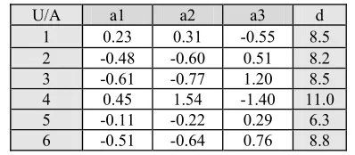
Example 2.

The data in question concern modeling of the energy for unfolding of a protein (tryptophan synthase alpha unit of the bacteriophage T4 lysosome), where 6 coded amino acids (AAs) are objects. The AAs are described in terms of seven attributes: a1=PIE and a2=PIF (two measures of the side chain lipophilicity), a3=DGR=∆G of

transfer from the protein interior to water, a4=SAC=surface area, a5=MR=molecular refractivity, a6=LAM=the

side chain polarity and a7=Vol=molecular volume.

(6)

R be a general relation defined as follows:

xRy iff |a(x)-a(y)| ≤ 0.5, where x,yU.

Table (2)

Original information system;

Condition attributes={a1, a2,a3}, decision attribute={d}.

U/A a1 a2 a3 d

1 0.23 0.31 -0.55 8.5

2 -0.48 -0.60 0.51 8.2

3 -0.61 -0.77 1.20 8.5

4 0.45 1.54 -1.40 11.0

5 -0.11 -0.22 0.29 6.3

6 -0.51 -0.64 0.76 8.8

From Table (2), we get:

The relation R with respect to a1 is: 1R={1,4,5}, 2R={2,3,5,6}, 3R={3,2,5,6}, 4R={4,1}, 5R={5,1,2,3,6}, 6R={6,2,3,5}.

Sub-base of topology Sa1 is:

S a1={{1,4,5},{2,3,5,6},{1,4},{1,2,3,5,6}}.

Base of topology β a1 is

β a1={Ф,{1,4,5},{2,3,5,6},{1,4},{1,2,3,5,6},{5},{1,5},{1}}.

Then the topology τ a1 is:

τ a1={U,Ф,{1},{5},{1,5},{1,4},{1,4,5},{2,3,5,6},{1,2,3,5,6}}.

And the complement of topology  a1 is:

τ a1c = a1=

{Ф,U,{2,3,4,5,6},{1,2,3,4,6},{2,3,4,6},{2,3,5,6},{2,3,6},{1,4},{4}}. U/IND({D}={{1, 3},{2},{4},{5},{6}}

Y1={1,3}, Y2={2}, Y3={4}, Y4={5}, Y5={6}

S

Y1={1},

S

Y2=Ф,

S

Y3=Ф,

S

Y4={5},

S

Y5=Ф

1

S_POS({a },D) =

{1,5}

1 1

|| _

({ }, ) ||

2 1

||

6

3

S a

S

POS a

D

r

U



 

S a2={{1},{2,3,5,6},{3,2,6},{4},{5,6,2}}.

β a2={Ф, {1},{2,3,5,6},{3,2,6},{4},{5,6,2},{2,6}}

τ a2={Ф, U,{1},{2,3,5,6},{3,2,6},{4},{5,6,2},{2,6},{1,2,3,5,6},{1,2,3,6}

{1,4},{1,2,5,6},{1,2,6},{2,3,4,5,6},{2,3,4,6},{2,4,5,6},{2,4,6}} And the complement of topology  a1 is:

τ a2c = a2={ U, Ф,{2,3,4,5,6},{1,4 },{1,4,5},{1,2,3,5,6},{1,3,4},{1,3,4,5},

{4},{4,5},{2,3,5,6},{3,4},{3,4,5},{1},{1,5},{1,3},{1,3,5}} U/IND({D}={{1, 3},{2},{4},{5},{6}}

Y1={1,3} Y2={2} Y3={4} Y4={5} Y5={6}

S

Y1={1}

S

Y2=Ф

S

Y3={4}

S

Y4= Ф

S

Y5=Ф

2

(7)

2 2

|| _

({ }, ) ||

2 1

||

6

3

S a

S

POS a

D

r

U



 

S a3={{1},{2, 5,6},{3,6},{4},{6,2,3,5}}.

β a3={Ф, {1},{2, 5,6},{3,6},{4},{6,2,3,5},{6}}.

τ a3={Ф, U, { 1},{2, 5,6},{3,6},{4},{6,2,3,5},{6},{1,2,5,6},{1,3,6},{1,4},{1,2,3,5,6},

{1,6},{2,4,5,6},{3,4,6},{2,3,4,5,6},{4,6}} And the complement of topology  a3 is:

τ a3c = a3={ U, Ф,{2,3,4,5,6},{1,3,4 },{1,2,4,5},{1,2,3,5,6},{1 ,4},{3,4},{2,4,5}

,{2,3,5,6},{4},{1,3},{1,2,5},{1},{1,2,3,4,5},{2,3,4,5},{1,2,3,5}} U/IND({D}={{1, 3},{2},{4},{5},{6}}

Y1={1,3} Y2={2} Y3={4} Y4={5} Y5={6}

S

Y1={1}

S

Y2=Ф

S

Y3={4}

S

Y4= Ф

S

Y5=Ф

3

S_POS({a },D) =

{1,4}

3 3

|| _

({ }, ) ||

2

1 ||

||

6

3

S a

S

POS a

D

r

U



 

Then Red=A

Note: We can use minimal base and its complement for calculating semi open sets instead of using the topology and its complement for simplification. See the following example.

Example 3.

Medical Application:

10 female patients had positive history of CTS and positive Tinel's test, then U={1,2,3,4,5,6,7,8,9,10} The attributes are different factors (personal factors "age, site, duration" and sensor conduction presentation factors "SCV,SA") , then A={SCV,SA,Age,Site,Duration}={a1,a2,a3,a4,a5} respectively.

As shown in Table (3)

Table (3) Pt. N0.

SCV m/s

SA

v AGE Year SITE Rt,Lt DURATION Month

a1 a2 a3 a4 a5

1 29.9 20 23 Rt 5

2 30.8 35 22 Rt 2

3 30.9 7 33 Rt 10

4 33.3 19.3 28 Rt 8

5 22.2 11.7 32 Rt 7

6 42.8 19 27 Lt 5.5

7 20.8 8.76 32 Rt 10

8 31.7 33.3 40 Lt 9.5

9 19 11 38 Rt 11

10 37.3 17.3 45 Rt 9.5

(8)

The relation R with respect to a1 is: 1R={1,2,3,8}, 2R={2,1,3,,8}, 3R={3,1,2,8}, 4R={4,8}, 5R={5,7},

6R={6},7R={7,5,9},8R={8,1,2,3,4},9R={9,7},10R={10}. Subbase of topology Sa1 is:

S a1={{1,2,3,8},{4,8},{5,7},{6},{5,7,9},{1,2,3,4,8},{7,9},{10}}.

Minimal Base of topology β a1 is

β a1={Ф, {1,2,3,8},{4,8},{5,7},{6},{7,9},{10},{8},{7}}.

The complement of minimal base is: β a1c= {U,{4,5,6,7,9,10},{1,2,3,5,6,7,9,10},

{1,2,3,4,6,8,9,10},{1,2,3,4,5,7,8,9,10},{1,2,3,4,5,6,8,10},{1,2,3,4,5,6,7,8,9},{1,2,3,4,5,6,7,9,10},{1,2,3,4,5,6,8, 9,10}}

The relation R with respect to all attributes A:

1R={1}, 2R={2}, 3R={3}, 4R={4}, 5R={5}, 6R={6}, 7R={7}, 8R={8}, 9R={9}, 10R={10}. S A={{1},{2},{3},{4},{5},{6},{7},{8},{9},{10}}

Y1={1} Y2={2} Y3={3} Y4={4}Y5={5} Y6={6} Y7={7} Y8={8} Y9={9} Y10={10}

S

Y1= Ф

S

Y2= Ф

S

Y3= Ф

S

Y4= Ф

S

Y5=Ф

S

Y6= {6}

S

Y7= {7}

S

Y8={8}

S

Y9=Ф

S

Y10={10}

1 1

|| _

({ }, ) ||

4

0.4 ||

||

10

S a

S

POS a

A

r

U



The relation R with respect to a2 is: 1R={1,4,6}, 2R={2,8}, 3R={3,7}, 4R={4,1,6,10}, 5R={5,9},

6R={6,1,4,10}, 7R={7,3}, 8R={8,2}, 9R={9,5}, 10R={10,4,6}.

S a2={{1,4,6},{2,8},{3,7},{1,4,6,10},{5, 9},{4,6,10}}

β a2={Ф, {1,4,6},{2,8},{3,7},{5, 9},{4,6,10},{4,6}}.

But S A={{1},{2},{3},{4},{5},{6},{7},{8},{9},{10}}

Y1={1} Y2={2} Y3={3} Y4={4}Y5={5} Y6={6} Y7={7} Y8={8} Y9={9} Y10={10}

S

Y1= Ф

S

Y2= Ф

S

Y3= Ф

S

Y4= Ф

S

Y5=Ф

S

Y6= Ф

S

Y7= Ф

S

Y8= Ф

S

Y9=Ф

S

Y10= Ф

2 2

|| _

({ }, ) ||

0

0 ||

||

10

S a

S

POS a

A

r

U



The relation R with respect to a3 is: 1R={1,2}, 2R={2,1}, 3R={3,5,7}, 4R={4,6}, 5R={5,3,7}, 6R={6,4},

7R={7,3,5}, 8R={8,9}, 9R={9,8}, 10R={10}.

S a3={{1,2},{3,5,7},{4,6},{8,9},{10}}

Minimal Base of topology β a3is

β a3={Ф, {1,2},{3,5,7},{4,6},{8,9},{10}}

But S A={{1},{2},{3},{4},{5},{6},{7},{8},{9},{10}}

Y1={1} Y2={2} Y3={3} Y4={4}Y5={5} Y6={6} Y7={7} Y8={8} Y9={9} Y10={10}

S

Y1= Ф

S

Y2= Ф

S

Y3= Ф

S

Y4= Ф

S

Y5=Ф

S

Y6= Ф

S

Y7= Ф

S

Y8= Ф

S

Y9=Ф

S

Y10= Ф

3 3

|| _

({ }, ) ||

0

0 || ||

10

S a

S

POS a

A

r

U



(9)

1R=2R=3R=4R=5R=7R=9R=10R={1,2,3,,4,5,7,9,10}, 6R=8R={6,8} S a4={{1,2,3,4,5,7,9,10},{6,8}}

Minimal Base of topology β a4is β a4={Ф, {1,2,3,4,5,7,9,10},{6,8}}

But S A= {{1},{2},{3},{4},{5},{6},{7},{8},{9},{10}}

Y1={1} Y2={2} Y3={3} Y4={4}Y5={5} Y6={6} Y7={7} Y8={8} Y9={9} Y10={10}

S

Y1= Ф

S

Y2= Ф

S

Y3= Ф

S

Y4= Ф

S

Y5=Ф

S

Y6= Ф

S

Y7= Ф

S

Y8= Ф

S

Y9=Ф

S

Y10= Ф

4 4

|| _

({ }, ) ||

0

0 ||

||

10

S a

S

POS a

A

r

U



The relation R with respect to a5 is:

1R={1,5,6}, 2R={2}, 3R={3,4,7,8,9,10}, 4R={4,3,5,7,8,10}, 5R={5,1,4,6}, 6R={6,1,5}, 7R={7,3,4,8,9,10}, 8R={8,3,4,7,9,10}, 9R={9,3,7,8,10}, 10R={10,3,4,7,8,9}.

Sa5={{1,5,6},{2},{3,4,7,8,9,10},{3,4,5,7,8,10},{1,4,5,6},{3,7,8,9,10}}

βa5={Ф,{1,5,6},{2},{3,4,7,8,9,10},{3,4,5,7,8,10},{1,4,5,6},{3,7,8,9,10},{5},{3,4,7,8,10},{4},{4,5},{3,7,8,10}}

But S A={{1},{2},{3},{4},{5},{6},{7},{8},{9},{10}}

Y1={1} Y2={2} Y3={3} Y4={4}Y5={5} Y6={6} Y7={7} Y8={8} Y9={9} Y10={10}

S

Y1= Ф

S

Y2= {2}

S

Y3= Ф

S

Y4= {4}

S

Y5={5}

S

Y6= Ф

S

Y7= Ф

S

Y8= Ф

S

Y9=Ф

S

Y10= Ф

5 5

|| _

({ }, ) ||

3

0.3 || ||

10

S a

S

POS a

A

r

U



Then Red=A-{a2,a3,a4}={a1,a5}

6. Conclusion

The semi rough set correlation factor give us the correlation factor between attributes and can be used for reduction of information system tables according to the value of semi correlation factor.

References

[1] Abo Khadra A.A., and Ali M. E., "Rough Sets and Correlation Factors", international journal of institute mathematics and

computer science, 19(1), June 2008.

[2] Hogg, R. V. and Craig, A. T., "Introduction to Mathematical Statistics", 5th ed. New York: Macmillan, 1995.

[3] Hu, X., Cercone N., Han, J., Ziarko, W, "GRS: A Generalized Rough Sets Model", in Data Mining, Data Mining, Rough Sets

and Granular Computing, T.Y. Lin, Y.Y.Yao and L. Zadeh (eds), Physica-Verlag, 447- 460, 2002.

[4] John L. Kelley. "General Topology", Springer-Verlag. ISBN 0-387-90125-6, 1975.

[5] Lin T.Y., "From rough sets and neighborhood systems to information granulation and computing in words", Proceedings of

European Congress on Intelligent Techniques and Soft Computing, 1602-1607, 1997.

[6] Lin T.Y., "Granular computing on binary relations I: data mining and neighborhood systems, II: rough set representations and

belief functions", In: Rough Sets in Knowledge Discovery , Lin T.Y., Polkowski L., Skowron A., (Eds.). Physica-Verlag, Heidelberg ,107-140, 1998.

[7] Lin T.Y., Yao Y.Y., Zadeh L.A., (Eds.) " Rough Sets, Granular Computing and Data Mining", Physica-Verlag, Heidelberg,

2002.

[8] Pawlak Z., "Rough Sets", International Journal of Information and computer Science, 11(5):341-356, 1982.

[9] Pawlak Z., "Rough Sets - Theoretical Aspects of Reasoning about data.", Kluwer Academic Publishers, Dordrecht, Boston,

London, 1991.

[10] Pawlak Z., Rough set approach to knowledge-based decision support, European Journal of Operational Research 99, 48-57,

1997.

[11] Polkowski, L., Skowron, A., "Rough mereology", Proc. ISMIS, Charlotte, NC, 85-94, 1994.

(10)

15(4), 333-365, 1996.

[13] Skowron, A., Stepaniuk, J., "Tolerance approximation spaces", Fundamenta Informaticae, 27(2-3), 245-253, 1996.

[14] Yee Leung, Manfred M. Fischer, Wei-Zhi Wu, Ju-Sheng Mi, "A rough set approach for the discovery of classification rules in

interval-valued information systems", International Journal of Approximate Reasoning, Volume 47, Issue 2, Pages 233-246, 2008.

[15] Yuhua Qian, Jiye Liang, Chuangyin Dang , "Converse approximation and rule extraction from decision tables in rough set

theory", Computers & Mathematics with Applications, Volume 55, Issue 8, Pages 1754-1765, 2008.