GSJ: Volume 7, Issue 9, September 2019, Online: ISSN 2310-9186
www.globalscientificjournal.com
A
S
TUDY
O
F
T
HE
S
TABILITY
O
F SLOPES
O
F
A
R
AILWAY
L
INE
:
A
BUJA
R
AIL
M
ASS
T
RANSIT
P
ROJECT
B
ETWEEN
L
OT
1
(K
UBWA
)
A
ND
L
OT
3
(C
ENTRAL
B
USINESS
D
ISTRICT
),
A
S
A
C
ASE
S
TUDY
Mbaezue, D. N.
1, Maduka, Fidelia I.
21,2 (Department of Civil Engineering, University of Abuja, Nigeria).
1donaz11@yahoo.com; 2fidesmind2000@yahoo.com
KeyWords
Slope stability Analysis, Critical Failure Surface, Slope Failure, Factor of Safety, Cut Slope, Limit Equilibrium Method, Shear Strength Parame-ters c and ɸ, Stability Number Method
ABSTRACT
1.0 Introduction
Slopes are found in Civil Engineering, principally in the design and construction of hydraulic structures and transportation infrastruc-tures.
Slope stability is the resistance of inclined surface to failure by sliding or collapsing. It is performed to assess the safe design of hu-man-made or natural slopes (examples: embankments, road cuts, open-pit mining, excavations, landfills etc.) and the equilibrium conditions.The main objectives of slope stability analysis are finding endangered areas, investigation of potential failure mechanisms, designing of optimal slopes with regard to safety, reliability and economics, designing possible remedial measures, e.g. barriers and stabilization *1+.
Slope failure due to slope instability in highway and railway infrastructures is a natural disaster that can endanger human lives and properties. It can negatively affect the economic growth of any country due to inefficient movement of goods, raw materials and services across the country. Frequent failures can also affect investor decision. Extra expenditure is incurred in the repair of the failed slope.
Among other common forms of slope failures, which are slip failure, slide failure, creep failure, failure due sinking into soft soil caused by excessive settlement and failure by plastic squeezing of soil and heaving of ground surface when water content exceeds the plastic limit of the soil *2+. However the most common mode of failure is slipping of an embankment or cutting. Considerable research work has been carried out into the causes of such failure. Through the results of various research collated, it has been es-tablished that water is frequently the cause of earth slips. It occurs either by eroding of the soil layer or by an increase of the mois-ture content of the soil resulting in the decrease of shear strength.
Water increases the disturbing moment on the soil by increasing the weight of the soil. This causes failure when the ratio of the re-sisting moment developed due to the shear strength of the soil to the disturbing moment induced by the shear stress on the soil is less than the specified factor of safety for failure to never occur. The ratio of the resisting moment to the disturbing moment is the factor of safety of the slope. “The purpose of slope stability analysis is to provide a quantitative measure of the stability of a slope or part of a slope. Traditionally, it is expressed as the factor of safety against failure of that slope *3+."
Owing to the damages caused by unstable slopes, the planning, design and construction of slopes along a highway or railway re-quires thorough geotechnical studies on representative soil samples of the proposed and existing slopes in order to determine their sustainability, suitability and stability. This study will determine the stability of the existing Abuja railway slopes. It will be achieved through the geotechnical analysis of representative soil samples of the existing slopes.
Analyses will be done to determine the factor of safety of the existing slopes. The higher the factor of safety of the representative soil of each slope, the higher the chances that the slope will not fail.
2.0 Materials and Methods
2.1 Site Visit and Description of Study Area
Abuja Rail Mass Transit commonly known as Abuja Light Rail is a light rail transport system in Abuja in the Federal Capital Territory, FCT, Nigeria. It is the first of its kind in the country and in West Africa and second such system in sub-Saharan Africa (after Addis Aba-ba Light Rail). It is 27 kilometres long with 8 stations, connecting the Abuja city center to the Abuja International airport and also connecting to the Federal Abuja-Kaduna line *4+.It is characterized by both cut and fill slopes along the railway line.
FIG. 1a: Project Site FIG.1b: Project Site with Herringbone System of Drainage
2.2 Soil Sampling and Investigations 2.2.1 Soil Sampling
Disturbed and undisturbed soil samples, representatives of the case slopes, were collected from the slopes at different locations. Undisturbed methods of sampling provide samples with comparable condition to the site conditions. Disturbed soil samples do not retain the in-situ properties of the soil during the collection process *5+.
2.2.2 Laboratory Investigations
Four test samples were investigated at Soilmen Engineering Services Ltd, Nigeria. The main purpose of the investigations was to de-termine the relevant material parameters required for slope stability evaluation. Representative soil samples were taken at each of kilometres 2, 3 and 4, for geotechnical investigation. The soils were classified and shear parameters obtained from direct shear box tests. The investigated shear strength parameters c and from the representative soil samples which are keys in the slope stability analysis were obtained.
Since the direct shear tests are mostly conducted for sandy or sandy lean clay or silt material and by classification the soil on slopes under study are silty clay materials. This necessitated the use of the drained direct shear test result to ascertain the stability of the slopes.
2.3 Stability Analysis Procedure
The process of evaluating slope stability involves the following procedure:
a. Explore and sample foundation and borrow sources.
b. Characterize the soil strength by determining the shear strength parameters.
c. Establish the 2-D idealization of the cross section, including the surface geometry and the subsurface
d. Select trial slip surfaces and compute factors of safety using the selected method.
e. Repeat step (d) above until the “critical” slip surface has been located. The critical slip surface is the one that has the lowest factor of safety and which, therefore, represents the most likely failure mechanism.
2.4 Methods of Stability Analysis
Analysis of slopes has been carried out by limit equilibrium (LE) methods. The stability analyses were performed manually using the Taylor's Stability Number Method for cohesive and frictional soils. The result obtained by the above named methods was verified with a spread sheet solution for slope stability analysis using the Fellenius and Simplified Bishop Methods.
According to Aryal *7+, LE methods are important mainly because of two reasons. First, the methods have proved to be reasonably reliable in assessing the stability of slopes. Second, the methods require a limited amount of input, but can quickly perform an exten-sive trial-and-error search for the critical shear surface (CSS). He further states that “LE methods are missing the fundamental physics of stress-strain relationship, and thus they are unable to compute a realistic stress distribution”. In spite of this limitation, the LE methods are still common practice because of their simplicity and the reasonably accurate FOS obtained.
2.4.1 Taylor's Stability Number Method
The stability number method is also based on the premise that resistance of a soil mass to sliding results from cohesion and internal friction of the soil along the failure surface. A parameter called the stability number is introduced, which groups factors affecting the stability of soil slopes. The stability number (Ns) is defined as follows *8+.
Ns
Where unit weight of soil H height of cut C cohesion of soil
F factor of safety for cohesion and friction
In 1948, D. W. Taylor proposed a simple method of determining the minimum factor of safety for a slope in a homogeneous soil. Us-ing a total stress analysis and ignorUs-ing the possibility of tension cracks, he produced a series of curves which relate a stability number (N) to the slope angle β. For slope angles greater than 53o, the critical circle passes through the toe of the slope. For slope angles less than 53o the critical circle may pass in front of the toe *9+. Taylor's chart 1 is principally used forɸ=0 soils while Taylor's chart 2 is mainly used for ɸ>0 soils.
2.4.3 The Simplified Bishop Method
The Simplified Bishop Method was developed by Bishop (1955). This procedure is based on the assumption that the interslice forces are horizontal, as shown in below.
A circular slip surface is also assumed in the Simplified Bishop Method. Forces are summed in the vertical direction. The resulting equilibrium equation is combined with the Mohr-Coulomb equation and the definition of the factor of safety to determine the forces on the base of the slice. Finally, moments are summed about the center of the circular slip surface to obtain the following expression for the factor of safety 6:
FIG 3: Simplified Bishop Method of slices 6
F
Where Δx is the width of the slice, and mα is defined by the following equation,
m cos
Where
c' and ’ = shear strength parameters for the center of the base of the slice W = weight of the slice
Α = inclination of the bottom of the slice
u = pore water pressure at the center of the base of the slice
Δx = length of the bottom of the sliceα = inclination of the bottom of the slice P = resultant water force acting perpendicular to the top of the slice
Β = inclination of the top of the slice
MP = moment about the center of the circle produced by the water force acting on the top of the slice R = radius of the circle.
Because the value of the term m depends on the factor of safety, the factor of safety appears on both sides of Equation. Equation cannot be manipulated such that an explicit expression is obtained for the factor of safety. Thus, an iterative, trial and error proce-dure is used to solve for the factor of safety 6.
2.4.3 Fellenius method
In this method, the forces on the sides of the slice are neglected. The normal force on the base of the slice is calculated by summing forces in a direction perpendicular to the bottom of the slice. Once the normal force is calculated, moments are summed about the center of the circle to compute the factor of safety. For a slice and the forces shown in Figure below, the factor of safety is computed from the equation *6+.
F
Where
c' and φ’ = shear strength parameters for the center of the base of the slice
W = weight of the slice
α = inclination of the bottom of the slice
u = pore water pressure at the center of the base of the slice
∆l = length of the bottom of the slice
3.0 Stability Analysis of Case Study
Table 1: Summary of Laboratory Test Results
Test Location (Km) c (KN/m2) ɸ (degree) γb (Kg/m3)
Direct Shear Box 2 15.1 35.9 1815
Direct Shear Box 3 11.0 35.6 1838
Direct Shear Box 4 12.8 34.4 1868
γ= total unit weight of soil KN/m2; c= effective cohesion KN/m2; ɸ= effective angle of internal friction in degree; β= angle of slope; H= height of slope; FOS= factor of safety; γb= bulk density of soil in Kg/m3.
Table 2: Safety Factor Design Significance *8+
Safety Factor
Significance
Less than 1.0
Unsafe
1.0 to 1.2
Questionable safety
1.3 to 1.4
Satisfactory for cuts, fills; questionable for
dams
1.5 to 1.75
Safe for dams
3.2 Analysis of Slope Using the Limit equilibrium Methods of Slope Analysis. 3.2.1 Slope on KM 2
1:1.5
7.34m 1.9m
β
Railway Line
Main Drain
FIG.5
:
Cross Section of Slope at Kilometre 2Using the Stability Number Method *12+:
Slope Height, H=7.34m
Slope =1:1.5
Slope angle β= tan-1 (1/1.5) = 34o
c=15.1 KN/m2, ɸ= 35.9o
γ = 1815×9.81/1000 = 17.81KN/m2
FOS =Fs =Fc
ɸdeveloped = ɸ/FS = 35.9o / 1.5 =23.93
Thus *ɸd, β+ = *23.93, 34o+
From Taylor’s chart (FIG. 2b),Stability Number, Ns = 0.02
Ns = C/γHFS or H = C/NsγFS
H = 15.1/ (0.02×17.81×1.5)
H= 28.26m
Thus the assumed slope height, 28.6m, is greater than the actual slope height, 7.34m, implying that the actual FOS is higher than 1.5 assumed; hence, a higher value of FOS must be tried*12+.
Try FOS = 2.0
FOS = Fs = Fc; ɸd = 35.9/2.0 = 17.95
With ɸd=17.95 and β = 34o, from Taylor's stability chart (FIG. 2b) Stability Number, Ns= 0.045
H= 15.1/ (0.045×17.81×2.0)
H = 9.42m
Because the assumed slope height 9.42m and the actual slope height 7.34m are still not the same, a higher value of FOS must be tried.
Try FOS=2.2
Hence *ɸd, β+ = *16.34, 34o+
With ɸd=16.34 and β = 34o, Stability Number, Ns=0.053
H= 15.1/ (0.053×17.81×2.2)
H =7.27m; approximately, H= 7.30m.
Thus the computed height 7.30m is approximately close to the actual height of 7.34m.
Therefore the FOS is 2.2.
The slope is safe (see table 2, for safety factor design significance).
3.2.2 Slope at KM 3
1:5
9.26m
3.8
Railway Line
Main Drain
FIG 6: Cross Section of Slope at kilometre 3
Slope height H=9.26m
γ= 1838×9.81/1000=18.03KN/m2
c=11.0 KN/m2, ɸ= 35.6o
Try FOS =1.8
ɸdeveloped = ɸd= ɸ/FOS = 35.6o / 1.8 =23.93
Thus *ɸd, β+= *19.77, 34o+
From Taylor’s chart (FIG. 2b), Stability Number, Ns = 0.035
Ns = C/γHFS or H = C/NsγFS
H = 11.0/ (0.035×18.03×1.8) = 9.68m
Thus the assumed slope height, 9.68m, is greater than the actual slope height, 9.26m, implying that the actual FOS is higher than 1.8 assumed; hence, a higher value of FOS must be tried *12+.
Try FOS=1.85
Thus *ɸd, β+= *19.24, 34o+;from FIG 2b, Stability Number, Ns= 0.038
H= 11.0/ (0.038×18.03×1.85)= 8.68m
Thus the assumed slope height, 8.68m, is less than the actual slope height, 9.26m, implying that the actual FOS is lower than 1.85 assumed; hence, a lower value of FOS must be tried.
Hence, try FOS=1.75
Thus *ɸd, β+= *20.34, 34o+
Stability Number, Ns=0.034
H= 11/ (0.034×18.03×1.75)
H =10.25m
Try FOS=1.82
Thus *ɸd, β+= *19.56, 34o+; Stability Number, Ns=0.035
H= 11/ (0.035×18.03×1.82) =9.58m
The computed H =9.58 is close to the actual slope height of 9.26m; therefore, the factor of safety against failure is 1.82.
The slope is safe (see table 2, for safety factor design significance).
3.2.3 Analysis of slope on KM 4
7.01 1:5
4.80 Railway line
Main Drain
FIG. 7:Cross section of Slope at kilometre 4
Using the Stability Number Method *12+:
Slope height H=7.01m
γ = 1868×9.81/1000 = 18.33KN/m2
c=12.8 KN/m2, ɸ= 34.4o
Try FOS =2.2
ɸdeveloped= ɸ/FS = 34.4o / 2.2 =15.64
*ɸd, β+= *15.64, 34o+
From Taylor’s chart (FIG. 2b),Stability Number, Ns = 0.053
Ns = C/γHFS or H = C/NsγFS
H = 12.8/ (0.053×18.33×2.2)
H = 5.99m
Thus the assumed slope height, 5.99m, is less than the actual slope height, 7.01m, implying that the actual FOS is lower than 2.2 as-sumed; hence, a lower value of FOS must be tried.
Try FOS = 2.1
*ɸd, β+= *16.38, 34o+
Stability Number, Ns= 0.052
H= 12.8/ (0.052×18.33×2.1)
H = 6.39m
Because the assumed slope height and the actual slope height are still not the same value, another value of FOS must be tried.
Try FOS=2.07
Thus *ɸd, β+= *16.62, 34o+
Stability Number, Ns=0.048
H= 12.8/ (0.048×18.33×2.07)
H =7.03m
Try FOS=1.95
Thus *ɸd, β+= *17.64, 34o+
Stability Number, Ns=0.045
H= 12.8/ (0.045×18.33×1.95)
H = 7.96m
The computed H = 7.03m is close to the actual slope height of 7.01m; hence, the FOS against failure is 2.07.
3.0 Spread Sheet Solution
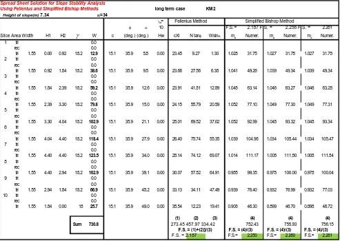
3.1 Table 3: Spread Sheet Solution of Slope at KM 2
Spread Sheet Solution for Slope Stability Analysis
Using Fellenius and Simplified Bishop Methods long term case KM 2
Height of slope(m) 7.34 = 34
w= Fellenius Method Simplified Bishop Method
10 F.S. = 2.187 F.S. = 2.256 F.S. = 2.261
Slice Area Width H1 H2 W c (deg.) (deg.) Hw cXl N tan Wsin ma Numer. ma Numer. ma Numer.
1 tri 0.0
rec 0.0
tri 1.55 0.00 0.92 18.2 12.9 15.1 35.9 5.8 0.00 23.45 9.27 1.30 1.028 31.75 1.027 31.78 1.027 31.78
2 tri 0.0
rec 0.0
tri 1.55 0.92 1.84 18.2 38.6 15.1 35.9 9.5 0.00 23.66 27.56 6.38 1.041 49.26 1.039 49.34 1.039 49.34
3 tri 0.0
rec 0.0
tri 1.55 1.84 2.39 18.2 59.2 15.1 35.9 12.6 0.00 23.91 41.81 12.89 1.048 63.14 1.046 63.27 1.046 63.28
4 tri 0.0
rec 0.0
tri 1.55 2.39 3.30 18.2 79.8 15.1 35.9 15.0 0.00 24.15 55.79 20.59 1.052 77.10 1.049 77.30 1.049 77.31
5 tri 0.0
rec 0.0
tri 1.55 3.30 4.04 18.2 102.9 15.1 35.9 21.1 0.00 25.01 69.52 37.02 1.052 92.99 1.048 93.32 1.048 93.34
6 tri 0.0
rec 0.0
tri 1.55 4.04 4.40 18.2 118.4 15.1 35.9 27.9 0.00 26.40 75.74 55.35 1.039 104.96 1.034 105.44 1.034 105.47
7 tri 0.0
rec 0.0
tri 1.55 4.40 4.40 18.2 123.5 15.1 35.9 34.0 0.00 28.14 74.12 69.07 1.014 111.17 1.008 111.80 1.008 111.84
8 tri 0.0
rec 0.0
tri 1.55 4.40 2.94 18.2 102.9 15.1 35.9 39.1 0.00 30.07 57.82 64.91 0.985 99.35 0.978 100.00 0.978 100.04
9 tri 0.0
rec 0.0
tri 1.55 2.94 1.84 18.2 66.9 15.1 35.9 45.2 0.00 33.13 34.11 47.49 0.939 76.40 0.932 76.99 0.932 77.03
10 tri 0.0
rec 0.0
tri 1.55 1.84 0.00 18 25.7 15.1 35.9 49.0 0.00 35.54 12.23 19.41 0.906 46.30 0.899 46.70 0.898 46.72
(1) (2) (3) (4) (4) (4)
Sum 730.8 273.45 457.97 334.42 752.43 755.93 756.15
F.S. = (1)+(2)]/(3) F.S. = (4)/(3) F.S. = (4)/(3) F.S. = (4)/(3)
3.2 Table 4: Spread Sheet Solution of Slope at KM 3
Spread Sheet Solution for Slope Stability Analysis
Using Fellenius and Simplified Bishop Methods long term case KM 3
Height of slope(m) 9.26 = 34
w= Fellenius Method Simplified Bishop Method
10 F.S. = 1.821 F.S. = 1.888 F.S. = 1.894 Slice Area Width H1 H2 W c (deg.) (deg.) Hw cXl N tan Wsin ma Numer. ma Numer. ma Numer.
1 tri 0.0
rec 0.0
tri 1.95 0.00 1.16 18.4 20.7 11.0 35.6 5.8 0.00 21.55 14.77 2.09 1.035 35.08 1.033 35.13 1.033 35.13
2 tri 0.0
rec 0.0
tri 1.95 1.16 2.32 18.4 62.2 11.0 35.6 9.5 0.00 21.74 43.93 10.29 1.051 62.77 1.049 62.90 1.049 62.92
3 tri 0.0
rec 0.0
tri 1.95 2.32 3.01 18.4 95.4 11.0 35.6 12.6 0.00 21.97 66.65 20.78 1.062 84.53 1.059 84.77 1.058 84.79
4 tri 0.0
rec 0.0
tri 1.95 3.01 4.17 18.4 128.6 11.0 35.6 15.0 0.00 22.20 88.93 33.19 1.068 106.30 1.064 106.66 1.064 106.70
5 tri 0.0
rec 0.0
tri 1.95 4.17 5.09 18.4 165.9 11.0 35.6 21.1 0.00 22.98 110.82 59.67 1.075 130.49 1.069 131.11 1.069 131.16
6 tri 0.0
rec 0.0
tri 1.95 5.09 5.56 18.4 190.8 11.0 35.6 27.9 0.00 24.26 120.73 89.21 1.068 147.99 1.061 148.91 1.061 148.99
7 tri 0.0
rec 0.0
tri 1.95 5.56 5.56 18.4 199.1 11.0 35.6 34.0 0.00 25.87 118.16 111.32 1.049 156.32 1.041 157.50 1.040 157.60
8 tri 0.0
rec 0.0
tri 1.95 5.56 3.70 18.4 165.9 11.0 35.6 39.1 0.00 27.63 92.17 104.63 1.024 136.92 1.015 138.12 1.014 138.22
9 tri 0.0
rec 0.0
tri 1.95 3.70 2.32 18.4 107.8 11.0 35.6 45.2 0.00 30.44 54.38 76.54 0.984 100.30 0.974 101.33 0.973 101.42
10 tri 0.0
rec 0.0
tri 1.95 2.32 0.00 18 41.5 11.0 35.6 49.0 0.00 32.66 19.50 31.28 0.953 53.65 0.943 54.25 0.942 54.30
(1) (2) (3) (4) (4) (4)
Sum 1177.9 251.31 730.03 539.00 1014.35 1020.67 1021.23
F.S. = (1)+(2)]/(3) F.S. = (4)/(3) F.S. = (4)/(3) F.S. = (4)/(3)
3.3 Table 5: Spread Sheet Solution of Slope at KM 4
Table 5: Summary of Stability Analysis Result
Spread Sheet Solution for Slope Stability Analysis
Using Fellenius and Simplified Bishop Methods long term case KM 4
Height of slope(m) 7.01 = 34
w= Fellenius Method Simplified Bishop Method
10 F.S. = 2.001 F.S. = 2.066 F.S. = 2.070 Slice Area Width H1 H2 W c (deg.) (deg.) Hw cXl N tan Wsin ma Numer. ma Numer. ma Numer.
1 tri 0.0
rec 0.0
tri 1.48 0.00 0.88 18.7 12.1 12.8 34.4 5.8 0.00 18.99 8.23 1.22 1.029 26.38 1.028 26.41 1.028 26.41
2 tri 0.0
rec 0.0
tri 1.48 0.88 1.75 18.7 36.2 12.8 34.4 9.5 0.00 19.15 24.47 5.99 1.043 41.90 1.041 41.98 1.041 41.98
3 tri 0.0
rec 0.0
tri 1.48 1.75 2.28 18.7 55.6 12.8 34.4 12.6 0.00 19.35 37.13 12.10 1.051 54.19 1.048 54.31 1.048 54.32
4 tri 0.0
rec 0.0
tri 1.48 2.28 3.15 18.7 74.9 12.8 34.4 15.0 0.00 19.55 49.54 19.33 1.054 66.54 1.052 66.72 1.051 66.73
5 tri 0.0
rec 0.0
tri 1.48 3.15 3.86 18.7 96.6 12.8 34.4 21.1 0.00 20.24 61.73 34.75 1.056 80.53 1.052 80.82 1.052 80.84
6 tri 0.0
rec 0.0
tri 1.48 3.86 4.21 18.7 111.1 12.8 34.4 27.9 0.00 21.37 67.25 51.96 1.044 90.97 1.039 91.41 1.039 91.45
7 tri 0.0
rec 0.0
tri 1.48 4.21 4.21 18.7 115.9 12.8 34.4 34.0 0.00 22.79 65.82 64.84 1.020 96.31 1.014 96.89 1.014 96.93
8 tri 0.0
rec 0.0
tri 1.48 4.21 2.80 18.7 96.6 12.8 34.4 39.1 0.00 24.34 51.34 60.94 0.992 85.74 0.985 86.34 0.985 86.38
9 tri 0.0
rec 0.0
tri 1.48 2.80 1.75 18.7 62.8 12.8 34.4 45.2 0.00 26.82 30.29 44.58 0.947 65.33 0.940 65.87 0.939 65.90
10 tri 0.0
rec 0.0
tri 1.48 1.75 0.00 19 24.2 12.8 34.4 49.0 0.00 28.77 10.86 18.22 0.915 38.73 0.907 39.08 0.906 39.10
(1) (2) (3) (4) (4) (4)
Sum 686.0 221.38 406.66 313.93 646.64 649.83 650.05
F.S. = (1)+(2)]/(3) F.S. = (4)/(3) F.S. = (4)/(3) F.S. = (4)/(3)
F.S. = 2.001 F.S.= 2.060 F.S.= 2.070 F.S.= 2.071
Slope
Location Spread Sheet Solution for Stability
Analysis Hand Calculation Method Stability of Slope Bishop Simplified Method Fellenius Method Stability No. Method Safe/Unsafe
KM2 2.250 2.187 2.20 Safe slope
KM3 1.882 1.821 1.82 Safe slope
3.4 Discussion of Results
Analyses carried out using the various named methods verified that the slopes under consideration are all stable with factors of safe-ty against failure not lower than 1.5. Generally, the Bishop method gives slightly higher factors of safesafe-ty than those calculated from the Fellenius Method *8+.From the spread sheet solutions, the factors of safety obtained using the Simplified Bishop Method were slightly higher than that obtained using the Fellenius Method.
For a stable slope, the slope angle β (angle of inclination) should not exceed the angle of internal friction ɸ; the geometric properties of the slopes satisfy this condition as shown in Table 1*8+.
The results of the study showed that the factor of safety of the slope does it increase or decrease with increase in values of cohesion c of the soil.
4.0 Conclusion and Recommendation
The limit equilibrium (LE) methods were used in this study to analyse the stability of existing cut slopes of the Abuja Rail Mass Transit pro-ject at the Central Business District, Abuja, Nigeria. The analyses were carried out using the Stability Number Method and verified using a spread sheet solution that applies the Fellenius and Simplified Bishop Methods of slices
.
Analyses carried out using the various named methods confirm that the slopes under consideration are all stable with factors of safety against failure not lower than 1.5.However, Conditions of a slope can be easily deteriorated within a certain period of time; to ensure continuous stability of slopes, the following safety measures are recommended:
1. Surface drains and sub-surface drains should be provided to drain water from the surface of the slopes and to maintain the ground water at a safe level.
2. Slopes may be protected by a rigid surface using sprayed concretes or by stone pitching to reduce rainwater infiltration and to prevent slope surface erosion.
3. The surface of slopes can also be protected by planting of vegetation, either grasses or trees. The type used is very much dependant on the angle of inclination of the slope (β). For slopes less than 35o, hydro seeding and pit planting of tress are recommended [13].
4. A cantilevered retaining wall may be designed and constructed at the toe of the slope on a deep pile foundation, to resist the active pressure of soil and the hydrostatic pressure that will develop behind the slope. A filter material should be pro-vided behind the retaining wall for easy flow of water and wipe holes should also be propro-vided on the walls to act as spill-way. This removes excess ground water into the main drain at the toe.
5. Counter weights should be provided at the toe to provide passive pressure, resisting force, to prevent movement. 6. The shear strength in a cutting diminishes with time and so does the factor of safety [9]; thus periodic inspection and
References
[1] (2019, September 17). Slope Stability Analysis. [online]. Available: https://en.wikipedia.org/wiki/Slope Stability Analysis.
[2] H. Niroumand, K. A. Kassim, A. Ghafooripour, R. Nazir and S. Y. Zolfeghari Far, "Investigation of Slope Failures in Soil Mechanics," Journal of Ge-otechnical Engineering, vol 17, pp 2701-2708, September 2012.
[3] Dr. R. Chitra and Dr M. Gupta, "International Journal Engineering Reseasrch & Technology (IJERT) ISSN: 2278-0181" geotechnical Investigations and
Slope stability Analysis of a Landslide, vol.5, pg 125, February-2016.
[4] (2019, June 10). Abuja Light Rail *online+. Available: https://en.wikipedia.org/wiki/Abuja_Light_Rail.
[5] T. Barnhart, "Disturbed vs. Undisturbed soil sampling" hunker.com, para. 2, September 20, 2018.[online]. Available: https://www.hunker.com/13406900/disturbed-vs-undisturbed-soil-sampling [Accessed: July 29, 2019].
[6] U.S. Army Corps of Engineers, Engineers Manual, Engineering and Design, Slopes Stability, Department of the Army, 2003.
[7] K. P. Aryal, “Slope Stability Evaluations by Limit Equilibrium and Finite Element Methods " Doctoral Thesis, Faculty of Engineering Science and Tech-nology, Norwegian University of Science and TechTech-nology, Trondheim, 2006, Accessed on: July 27, 2019.[online]. Available:
https://ntnuopen.ntnu.no/ntnu-xmlui/bitstream/handle/11250/231364/123392_FULLTEXT01.pdf?se.
[8] "Stability Analysis of Slopes" Scribd.com *online+. Available: https://www.scribd.com/document/414853804/Chohesive-Soil-Pg-9-42.
[9] R. Whitlow,”Basic Soil Mechanics”3rd ed.Addison Wesley, 1995. *E-book+ Available: http://www.civil.uwaterloo.ca.
[10] B. Trishna, "Stability of Earth Slopes in Soil Engineering" Soil Management.com*online+.
Available: http://www.soilmanagementindia.com/soil/slope-stability/stability-of-earth-slopes-soil-engineering/14489.
[11] M. Radoslaw,"Stability Charts for Uniform Slopes" Researchgate.com [online].
Available: https://www.researchgate.net/profile/Radoslaw_Michalowski
[12] Graduate Lectures in Geotechnical Engineering. CIE 725. Class Lecture, “The Stability of Earth Slopes.” Department of Civil Engineering, Universi-ty of Abuja, Abuja, Nigeria, 2018.