Sensor-Based Activity Recognition with Dynamically
Added Context
Jiahui Wen∗‡, Seng W. Loke, Jadwiga Indulska∗‡, Mingyang Zhong∗‡
∗The University of Queensland, School of Information Technology and Electrical Engineering, Australia
‡National ICT Australia (NICTA)
Department of Computer Science and Computer Engineering, La Trobe University, Australia
[email protected], [email protected], [email protected],
[email protected]
ABSTRACT
An activity recognition system essentially processes raw sen-sor data and maps them into latent activity classes. Most of the previous systems are built with supervised learning techniques and pre-defined data sources, and result in static models. However, in realistic and dynamic environments, original data sources may fail and new data sources be-come available, a robust activity recognition system should be able to perform evolution automatically with dynamic sensor availability in dynamic environments. In this paper, we propose methods that automatically incorporate dynam-ically available data sources to adapt and refine the recog-nition system at run-time. The system is built upon ensem-ble classifiers which can automatically choose the features with the most discriminative power. Extensive experimen-tal results with publicly available datasets demonstrate the effectiveness of our methods.
Categories and Subject Descriptors
H.4 [Information Systems Applications]: Miscellaneous
General Terms
Algorithms, Design, Experimentation, Performance
Keywords
activity recognition, extra context, activity adaptation
1.
INTRODUCTION
Sensor-based activity recognition has experienced its wide application in context-aware computing in the past decade, due to the important role it plays in everyday life. To name a few, recognizing human lifestyle can help to evaluate en-ergy expenditure [1]; monitoring human activity in smart homes enables just-in-time activity guidance provisioning
.
for elderly people and those suffering from cognitive defi-ciencies [4]; detecting walk and counting step can help to monitor elderly health [3].
State of the art activity recognition models usually rely on a static model, where only pre-defined data sources are considered while opportunistically available contexts which may potentially refine the systems are ignored. Here we argue that dynamically discovered context is also signifi-cant for the adaptation and refinement of activity models. For example, in [31], the authors demonstrate that addi-tional features such as vision features can help to improve the recognition accuracy for human activities, especially for static activities (e.g. sitting). Maekawa et al. [15] show in their work that, contextual information, such as the objects that the subjects interact with and the sound during the in-teraction, captured by camera and microphone can help to improve activity recognition performance. Extensive works prove that additional information such as location informa-tion [17], vital signs [11], readings from thermal sensor [6] and barometer [18] can also improve activity recognition ac-curacy.
Note that all the aforementioned extra data sources are specific to the post-deployment environment. Therefore, considering all the contextual information at the beginning of activity modelling is infeasible, due to the problem of data sparsity and the changes in the environment during post-deployment. Another motivation for our work is that sen-sors deployed for activity sensing are constantly broken and updated [14], so it is extremely important that the activity monitoring system can automatically evolve with the chang-ing environment. Our work is inspired by [7], where the authors propose an autonomic context management system which is able to populate dynamically discovered contextual information sources for automatic context provisioning. We state here that several challenges need to be addressed in order to achieve an activity recognition system that is able to incorporate dynamically discovered context. First, incor-porating new data sources would change the feature dimen-sionality, the pre-learned activity model should be flexible enough to allow for increment and decrement of the fea-ture dimensionality. Second, the system should be able to automatically identify the context that have the discrimina-tive power, while ignore those with marginal discriminadiscrimina-tive power. Furthermore, as model refinement with dynamically available context usually requires the labels of the new exam-ples to point out the direction of model adaptation, asking the user for the true labels is obtrusive. Therefore, selecting
MOBIQUITOUS 2015, July 22-24, Coimbra, Portugal Copyright © 2015 ICST
the most profitable and informative examples for adaptation is still challenging.
In this paper, we propose such an activity recognition sys-tem that addresses the aforementioned challenges. We prac-tically analyze and choose a machine learning model that is flexible with the change of feature dimensionality and can automatically identify the most discriminative features. In order to retrain and adapt the activity model by incorpo-rating the information provided by dynamically discovered data sources, we propose a method to choose the profitable examples without human intervention. Finally, we exploit temporal patterns of human behaviour and leverage graph-ical models to further improve the recognition performance. To conclude, this paper makes the following contributions.
1. We propose an activity recognition framework that can automatically incorporate dynamically discovered dis-criminative contexts, so as to improve activity recognition performance.
2. We propose a method that chooses the profitable and informative examples (incorporating discovered context) to retrain and adapt activity models without human interven-tion. We also propose a novel way of combining basic clas-sifier (i.e., AdaBoost) with graphical models (i.e. Hidden Markov model and Conditional Random Field) in order to exploit the temporal information to improve the recognition accuracy.
3. We demonstrate our system with three publicly avail-able datasets and analyze its effectiveness through compre-hensive experimental and comparison studies. We also in-vestigate the conditions under which the opportunistically discovered context is beneficial to recognition performance. It should be noted that in this paper, we choose iner-tial sensor (i.e. accelerometer, gyroscope) data as an exam-ple, but our methods can be easily extended to other data sources, as we do not make assumptions on the sensor data type, so any kind of sensors (e.g. inertial sensors, binary sensors, microphone, camera) can be used because the Ad-aBoost approach adopted in this paper can deal with both numeric and categorical features [13]. In addition, we do not distinguish the concepts of new data sources, new fea-tures and new contexts. Since new data source and context can be seen as dynamically discovered information from the viewpoint of the whole system, while feature is from the viewpoint of the classifier. The remainder of this paper is organized as follows. In Section 2, we discuss related work. In Section 3, we briefly describe the system overview and architecture of our activity model, and detail each compo-nent in Section 4. Section 5 reports the experimental results and analysis, followed by Section 6 where we conclude this paper with a summary.
2.
RELATED WORK
Activity recognition [27, 26] is not a new topic, especially with the proliferation of smartphones where on-board sen-sors such as GPS, camera, microphone, accelerometers and gyroscope, provide unprecedented opportunities for recog-nizing wide variety of human behaviours [10]. However, most of the state-of-the-art activity models are built upon static machine learning models, the reader is referred to [28] for more details.
Considering new context in dynamic environments to re-train and refine the activity model relates to model person-alization and semi-supervised learning from the viewpoint
of operation. Activity personalization adapts the general model to a specific user giving his/her data, while semi-supervised learning trains recognition models with labeled and unlabeled data. To name a few, Zhao et al. [32] pro-pose a cross-people activity recognition algorithm for per-sonalized activity-recognition model adaptation by integrat-ing a decision tree and the k-means clusterintegrat-ing algorithm. The predictions given by decision tree are re-organized by K-means, based on which the decisive thresholds in the tree are re-estimated. In [16], the authors train a classifier for each user. The ensemble classifiers are then weighted based on the error they make using the target user’s data. While in the semi-supervised area, unlabelled examples classified with high confidence are added to the training dataset to retrain and refine the model. Examples are self-training, co-training [21] and label propagation [20]. The problem of aforementioned methods is that only high-confidence exam-ples are considered, due to the fact that they can minimize the entropy [5]. However, high-confidence examples are less informative and make less contribution to the convergence of the model [21]. More importantly, those methods are built with statically defined input and are not suitable to cope with emerging context in dynamic environments.
Some other work leverage the knowledge-based method to deal with unseen data sources for activity recognition. For example, Tapia et al. [23] address the problem ofmodel in-completenessby leveraging external knowledge base to mea-sure the similarity between unseen features (object) and ex-isting features, so that they are able to obtain the probability of an unseen object given the activity classes. While in [25], the authors perform activity recognition based on the ob-ject usage and human actions. With no label for the action data, they use common sense knowledge to build an activity model by jointly training Dynamic Bayesian Network and Virtual AdaBoost. Those methods, however, rely heavily on existing knowledge to activity recognition. In this light, they are not applicable in the situation that we have no prior knowledge about dynamically discovered data sources.
Other research even perform activity recognition with dy-namic sensor selection. For example, in [8], the authors gen-erate multiple processing plans for the context to be moni-tored. The system dynamically updates the processing plans when sensors are newly registered or de-registered. In an-other work, Zappi et al. [30] introduce a scheme to dynam-ically select the sensor set for activity recognition in order to achieve the trade-off between accuracy and power. Since those work mainly focus on the aspect of energy-efficiency, they simply train each activity with all the available sensors, so that when the sensors are registered at runtime, the sys-tem already has the knowledge of how to post-process the sensor data, hence this limits the scalability of the system.
3.
FRAMEWORK
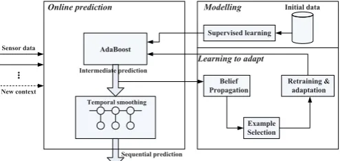
In this section, we will introduce our framework. The workflow of our system can be divided into three phases:
modelling, learning to adapt and online prediction. In the
modelling phase, an initial activity model is built with cur-rently available sensor data. As new data sources become dynamically available, we perform adaptation for the activ-ity model by considering the dynamic data sources in the
per-$GD%RRVW
%HOLHI 3URSDJDWLRQ
([DPSOH 6HOHFWLRQ
5HWUDLQLQJ DGDSWDWLRQ ,QLWLDOGDWD
6XSHUYLVHGOHDUQLQJ
1HZFRQWH[W 6HQVRUGDWD
6HTXHQWLDOSUHGLFWLRQ 7HPSRUDOVPRRWKLQJ ,QWHUPHGLDWHSUHGLFWLRQ
0RGHOOLQJ 2QOLQHSUHGLFWLRQ
/HDUQLQJWRDGDSW
Figure 1: Top level framework.
formance. It should be noted thatprediction is not the final stage. Instead, our system can keep looping between learn-ing to adaptandpredictionas long as discriminative context is discovered.
Modelling. We choose AdaBoost as our basic classifier, as it is lightweight enough for on-body devices and has been demonstrated to be robust for classification tasks [9]. The rationale for choosing AdaBoost also lies in the fact that it is flexible in the dimension of the feature space, and is able to automatically choose the most discriminative features in the training process.
Learning to adapt. When new data sources are dynami-cally discovered(the data sources can be discovered univer-sally with sensor modelling, the reader is referred to [7] for more details), the information they provide may be bene-ficial to improving the recognition accuracy. The goal of this stage is to perform adaptation for the activity models, so as to incorporate the information provided by the new data source (if it is discriminative enough). To achieve this, we perform belief propagation on the predictions given by AdaBoost and choose examples for retraining. The selected examples, which contain newly discovered context, are fed into AdaBoost to retrain and adapt the classifier.
Prediction. AdaBoost makes prediction individually and assumes no dependency between the posterior probability of neighbouring examples. We combine AdaBoost with graph-ical models to provide sequence predictions, as those models make temporal assumptions between adjacent predictions and are able to smooth out the outliers.
4.
METHODOLOGY
4.1
Basic modelling
Because of the special characteristics that meet out re-quirements, AdaBoost is selected as our basic classifier. The core of AdaBoost is to train an ensemble of weak classifiers and combine them to form a more robust and accurate clas-sifier. Each weak classifier makes decision based on a sin-gle feature and needs only be slightly better than random guessing. The final classifier is a linear combination of the weak classifiers, with each classifier weighted by the error it makes during the training process; more weight is given to the classifier that makes fewer errors.
As AdaBoost incrementally builds weak classifiers on the training dataset, it is more flexible in the dimensional changes of the feature space. When discriminative context is de-tected during thelearning to adapt phase, all AdaBoost has
to do is training a weak learner on the context and add it to the ensemble along with its weight, without the necessity to change the feature space and retrain the whole model. Also, in each iteration, AdaBoost only chooses the weak learner with minimum training error. In this light, it presents an effective and tractable way to automatically select the fea-tures with maximum discriminative power [12]. Therefore, it is not necessary to evaluate the discrimination of the new context manually.
As depicted in Algorithm 1, the AdaBoost learning al-gorithm takes as input the examples, the initial example weights and maximum iterations. The training of AdaBoost follows an iterative process. In each iteration, each weak learner is fitted to training dataset, and the one with the minimum weighted error is chosen (step 2). After that, the example weights are updated, so that more weights are given to the misclassified examples (step 4). During the next it-eration, the weak classifiers will focus more on those prob-lematic examples. The output of the training process is an ensemble of weak learners (step 6). Notice that in step 2, it trains a weak learner for each dimension of the feature space, but only selects the one with minimum weighted error. In this paper, we adopt decision stump as the weak learner, and then training weak learnerhkt(x) for dimension k is equiv-alent to finding the thresholdθkin that dimension to
min-imize the weighted error such thathk
t(xi) = hkt(xki) = 1 if xk
i > θk andhkt(xi) =−1 otherwise, where xki is the value
ofkthdimension of examplexi.
Algorithm 1AdaBoost.
Input:
Examples (x1, y1),· · ·,(xn, yn) where xi ∈ k a is
k-dimension feature vector,yi∈ {+1,−1};
Initial weight of n examplesD0(i) = 1/nfori= 1,· · ·, n; Weak learnersh(x)∈ {+1,−1};
Max iterationsT;
Output:
Ensemble of weak learners;
1: fort= 1 toT do
2: Find weak learnerht(x) that minimizes the weighted error:
ht(x) =argminhk t(x)
n
i=1Dt(i)I[hkt(xi)=yi]
t=ni=1Dt(i)I[ht(xi)=yi] ;
3: Compute the weight for the weak learner ht(x): αt =
1
2ln(1−tt);
4: Update the weight of examples: Dt+1(i) =
Dt(i)exp(−αyiht(xi))
iDt(i)exp(−αyiht(xi))fori= 1,· · ·, n; 5: end for
6: return H(x) =sign(Tt=1αtht(x));
AdaBoost is a discriminative classifier, and it performs classification by giving the definitive decision. This ap-proach has a potential problem that even if the classifier is uncertain with the class of the example, it chooses the class against which the example has the maximum evidence as the prediction. We argue that the posterior probability of an example is much more helpful, since it reflects the con-fidence in that prediction. This is important to the later stages such as the stage oflearning to adapt. To this end, we calculate the posterior probability for examples using the method from [12].
P(yi|xi) =
eψm(x)
eψm(x)+1 ifyi= +1 e−ψm(x)
e−ψm(x)+1 ifyi=−1
\N
\N
[N
[N
N N I
Xo \
I
N I N
Xo \
I \N
I
Figure 2: Belief propagation between hidden vari-able
where ψ is a constant and m(x) =
T
t=1αtht(x)
T
t=1αt . P(yi|xi) is thus regarded as the posterior distribution of examplexi.
Notice that the binary AdaBoost can be easily extended to multi-class classifiers by training a set of weak learners for each activity classito separate itself from others:
Hi(x) =
T
t=1
αi
thit(x) (2)
Accordingly, the prediction is made by argmaxi(Hi(x)) for a given examplex.
4.2
Belief propagation
As new sensors are dynamically discovered, we need to select examples that contain the new sensor data to adapt AdaBoost. The aim in this stage is to leverage belief prop-agation to smooth the outliers and rectify the results pro-duced by AdaBoost, so as to choose the most profitable and informative examples to learn the new context and adapt the activity model.
Due to the temporal characteristic of human behaviours, the current activity is more likely to be continued in the next time point than a new one. Therefore, there are strong cor-relations among the sequential predictions of the examples. It is apparent that AdaBoost makes no use of the tempo-ral information, since it assumes no dependencies among the examples, and performs classifications based solely on the local features. As a result, sensor noises or temporary interruption of the activities would certainly result in mis-classification.
Belief propagation is mainly performed for inference in graphical models, and in the form of message passing be-tween the nodes. The passing messages among the nodes are actually exerting influence from one variable to the oth-ers. In this light, the belief propagation is to send messages to the connected node and tell it what it should believe [29], and the hidden state of a node depends on not only local observations, but also the product of all incoming mes-sages from locally connected nodes.Upon convergence, the marginal distribution of the variable nodes can be approxi-mated with:
p(yk|X) = φf(yk)
f∈N(k)\fμf→k(yk)
yk φf(yk)
f∈N(k)\fμf→k(yk)
(3)
where φf(yk) is the local evidence, and μf→k(yk) is the message from neighbouring factor nodes for nodek, as shown in Figure 2.
In our scenario, the belief propagation is performed among the observation nodes and hidden nodes. The observation node at timetis the feature vector collected from the sen-sor data while the hidden node is the latent activity. Since
\N
\N \N \N
\N
[N
[N [N [N
[N
_ N N
S \ [
_ N N
S\ [
_ N N
S\ [
N _N
S \ [
N _N
S \ [
Figure 3: Belief propagation in our scenario. The
solid lines show the messages received by node k
from neighbouring four nodes.
the latent activity is unknown, the latent variableykis rep-resented in the form of a multinomial distribution over all the activities. The multinomial distribution is iteratively updated by incorporating the messages from not only local observations, but also adjacent nodes.
In our system, we only consider pairwise connections (Fig-ure 3) between the hidden nodes when performing belief propagation. Therefore, the messages that a node receives are the posterior probabilities of its neighbouring nodes based on their own local observations, as shown in (4)
p(yk|X) = p(yk|xk)
i∈N(k)\i:yi=ykp(yi|xi)
ykp(yk|xk)
i∈N(k)\i:yi=ykp(yi|xi)
(4)
Therefore, belief propagation is performed with an infer-ence step and followed by several iterative update steps. In the inference step, for each observation, AdaBoost gener-ates a posterior probability distribution over the hidden ac-tivities using Eq.(1). In the propagation step, those ini-tial estimations of posterior probabilities are propagated to neighbouring nodes. Those recipient nodeskthen combine the received probability distribution overyi together with
its local evidence given by AdaBoost and convert them into a distribution overyk, using Eq.(4). The iterative process can be repeated until convergence. In our experiment, we found that running belief propagation for only one iteration is sufficient to converge the posterior distribution.
The belief propagation is slightly modified in our imple-mentation. As the examples classified with high confidence usually tend to be the correct classification, we do not up-date the posterior distribution for those high-confidence ex-amples during the iterative process of belief propagation, so that their beliefs can be propagated to the uncertain exam-ples.
4.3
Examples selection
In this subsection, we introduce the method to select the examples for classifier retraining and adaptation. The exam-ples contain dynamically discovered context, and AdaBoost is able to automatically incorporate the new context if it is discriminative enough. In this way, AdaBoost can be self-adapted or -refined. We perform examples selection after the belief propagation for the sake of selecting the informative and profitable examples to quickly converge the classifier without human intervention.
4.3.1 Measurements
se-lected to adapt the model. The first metric we consider is the “drift” in the posterior distribution before and after the belief propagation. Belief propagation is able to smooth out the outliers by exploiting the temporal information. Those ex-amples that experience huge “drift” in their posterior distri-butions are much more valuable, since they are not modelled by the initial activity model and have a greater chance of residing near the classification boundaries. Jensen-Shannon divergence can be used to measure the “drift”, as it has been proved to be efficient to measure the distance between two distributions in previous work [22]. Supposingpiandqiare the posterior distributions of exampleibefore and after be-lief propagation respectively, and then the JS-divergence is:
JS(pi, qi) =1
2DKL(pi||m) + 1
2DKL(qi||m) (5)
where m = 12(pi+qi) andDKL(pi||m) = jpijlogpij
mj is the Kullback-Leibler divergence between two distributions. Therefore, we derive the first measurement as:
scorei1 = JS(pi, qi)−JSmin(p, q)
JSmax(p, q)−JSmin(p, q) (6)
we normalize the JS-divergence, so that the measurement based on the posterior distribution “drift” is always ranged in [0,1], in this way it is able to cater for characteristics of different activity data set.
As for the second measurement of profitability, we con-sider the number of consecutive neighbouring examples that have the same predicted results.
Ni=min(Nif orward, Nibackward)
scorei2= Ni−min(N)
max(N)−min(N)
(7)
where Nif orward and Nibackward are the number of consec-utive neighbouring observations that have the same predic-tions along the two direcpredic-tions of time series, from current observationi. It is normalized due to same reason asscorei1. This measurement shows the extent to which the neighbour-ing nodes have the consensus predictions, and the higher the number, the more likely that the prediction is correct. Ob-viously,scorei2 is proposed based on the temporal charac-teristic of human behaviour. One extreme condition is that the observation happens to be in the middle of an ongoing activity, and the scorei2 tends to be large and it is more confident about the prediction.
Finally, we consider the confidence of the examples after the belief propagation. The posterior distribution itself pro-vides the information about the confidence of an example. Adding the examples with the highest confidence is equiva-lent to locating the class center, which in turn also helps to adapt the model to some extent, even though those exam-ples are less informative. Therefore, the third measurement is formulated asscorei3=max(p(yi|xi)) (Eq.(4)).
To decide which example is more profitable, we need to take into account all the aforementioned metrics. There-fore, we determine the final score for the profitability of an example based on the corresponding scores for each of the metrics. The combined score is defined as follows:
scorei=α1scorei1+α2scorei2+α3scorei3
s.t.3
i=1
αi= 1 (8)
where the weightsαiis manually given. In our method, we evenly distribute the importance to the three metrics by set-tingα1=α2=α3. However, by giving different weights, the model may present different characteristics. For example, by increasingα3 we give more weight to the high-confidence examples, and then the model adapts conservatively and the convergence is quite slow. By contrast, when we put more weight toscorei1, the model only takes those exam-ples whose posterior distribution changes dramatically be-fore and after belief propagation, and then the adaptation is performed aggressively. There is a danger that noisy data may be added and the model is jeopardised.
4.3.2 Retraining
Upon selecting the examples for model adaptation, Ad-aBoost can automatically determine the discriminative power of the new context (if there is any) in the example, and dy-namically incorporate them for classification if they are dis-criminative enough. In this way, the model is adapted to new coming data.
One issue should be addressed when selecting the exam-ples, this is the amount of retraining data among different activity classes should be balanced during the adaptation process. During the experiment we found that for activ-ity class with small training dataset, the iterative process of training weak learners is unexpectedly terminated ear-lier. As a result, the trained ensemble of classifiers for that class overfit the small amount of data. That is the reason AdaBoost focuses more on training activities with unevenly large dataset [9]. Therefore, in this paper, we accumulate for each activity class the same amount of dataset before retraining.
4.4
Sequential prediction
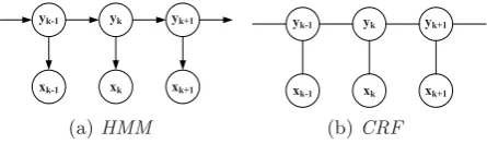
When the adapted AdaBoost is deployed for online predic-tion, we combine it with graphical models to further smooth outliers. Even though the basic idea behind this stage and belief propagation are both to exploit the temporal informa-tion among the activity data, belief propagainforma-tion is deployed for offline data analysis, sufficient data should be accumu-lated and analyzed for model adaptation (second stage in Figure 1), while graphical models cater for online lightweight predictions (third stage in Figure 1). Furthermore, belief propagation requires the posterior distribution to evaluate the profitability of the examples.
\N \N \N
[N [N
[N
(a)HMM
\N \N \N
[N [N
[N
(b)CRF
Figure 4: Graphical model of HMM and CRF.
that has maximum likelihood. Therefore, they do not model the transitions among different classes.
4.4.1 BoostHMM
In Hidden Markov models, the variables include hidden states and observations. As shown in Figure 4(a), it models the joint distribution of those variables by making Markov assumptions that current latent activityykonly depends on previous latent activityyk−1, while current observationxk depends on current latent activity, formulated as follows:
p(x,y) =p(y1)p(x1|y1)
K
k=2
p(yk|yk−1)p(xk|yk) (9)
where the emission probabilityp(xk|yk) can approximated
with the posterior distributionp(yk|xk) given by AdaBoost (Eq.(1)) using Bayes’ rule:
p(xk|yk) = p(yk|xk)p(xk)
p(yk) ∝p(yk|xk) (10)
where prior knowledgep(yk) is identical for different
activi-ties because we balance the training data over all the activity classes. For a variablexk that is observed at timek,p(xk) is a constant when calculating its evidence against different classes. Therefore, the emission probability is proportional to the posterior probability given by AdaBoost, and the joint distribution can be re-formulated as follows:
p(x,y)∝p(y1)p(y1|x1)
K
k=2
p(yk|yk−1)p(yk|xk) (11)
As for transition probability, we manually set the self-transition probabilities to be large to temporally smooth out the ac-tivities, and encourage them to continue unless observable evidence strongly suggests a different activity [25], denoted as follows:
p(yk|yk−1) =
1− yk=yk−1
otherwise (12)
we experimentally set to be 0.1 in our system, as it is demonstrated to be effective enough to achieve reasonable accuracy. Inferring the hidden states is equivalent to finding the sequences that maximize the joint probability depicted in Eq.(11), which can be performed by the Viterbi algorithm.
4.4.2 BoostCRF
In Conditional Random Field (CRF), the connections be-tween the variables denote the potentials bebe-tween them, and the potential functions map those potentials into real num-bers. Due to the flexible definition of the potential func-tions, CRF has various structures. In our system, we only consider linear-chain CRF (Figure 4(b)). Therefore, we need
to define local potential functions between observation and hidden node at each time step, and pairwise potential func-tions between consecutive hidden nodes. The conditional distribution can be formulated as:
p(y|x) = 1
Z(x)exp
K
k=1
λTf(y
k, yk−1, xk)
= 1
Z(x)exp
K
k=1
λT
sfs(yk, yk−1) +λTjfj(yk, xk)
(13)
wherefj(yk, xk) andfs(yk, yk−1) are the local and pairwise potential functions at timek. λsandλjare the correspond-ing weights. Z(x) is the normalization factor, formulated as
yexp Kk=1λkfk(yk, yk−1, xk)
.
Inspired by [13], we map the weak learners trained in Ad-aBoost to the local potential functions in CRF, while the weights of the potential functions are mapped to the weights of the weak learners. This is reasonable since more weights are given to the potential functions that can better explain the data, whereas weak learners with less error rate have a larger weight. Using Eq.(2), the weighted sum of local potential functions against activity classiis:
λT
jfj(yk, xk) = T
t=1
αi
thit(xk) (14)
However, mapping the weight of pairwise potential func-tion is non-trivial. To deal with this, we define pairwise potential function that characterize the temporal transition between activities:
fij(yk, yk−1) =
1 yk=i, yk−1=j
0 otherwise (15)
where potential functionfijcharacterize the transition from activityjto activityi. Assume that there is a weak learner
hi(y
k =i, yk−1 = j) in AdaBoost that can be mapped to the potential functionfij. Obviously, the error rate of the weak learner can be estimated from the training dataset by frequency counting:
ij= 1−expected number of transitions from j to i expected number of transitions out of j (16)
then according to Algorithm 1, the weight of the weak learner can be approximated as:
αij=1 2ln(
1−ij
ij ) (17)
the weight of weak learner hi(y
k = i, yk−1 = j), αij, is
5.
EXPERIMENT
In this section, we will validate our methods introduced in the previous sections. We firstly introduce the datasets, and then specify the method to evaluate our approach.
5.1
Datasets
Smartphone dataset (SD) [19]: Activity data was collected from accelerometer, gyroscope and magnetometer on an An-droid device worn in different body position (arm, belt, waist and pocket), when the subject performs standing, walking, upstairs, sitting, running and downstairs. The sample rate is set to be 50Hz. We compute time domain features such as mean, standard deviation, median, zero crossing rate, vari-ance, root mean square for each axis of the sensors with a 2 sec sliding window and 50% overlap.
Sensors activity dataset (SAD) [19]: Sensor data was col-lected when the 10 volunteers perform standing, walking, upstairs, sitting, downstairs, jogging and biking. We extract the same features as the first dataset.
UCI HAR dataset [2]: The dataset was collected with accelerometer and gyroscope from a Samsung Galaxy SII smartphone worn by 30 volunteers. The smartphone was fixed on the waist when the subjects perform six activi-ties (walking, walking upstairs, walking downstairs, sitting, standing, laying). The 561 features were computed based the sliding window of 2.56 sec and 50% overlap. In our experiment, we only consider time domain features, as it is computationally expensive to compute the frequency do-main features on the mobile phone during online prediction. Therefore, we have 80 features from the gyroscope and 120 features from the accelerometer.
5.2
Set up
To validate our system, each of the datasets is divided into three portions, in accordance with the three stages in Fig-ure 1. Specifically, we train the activity model with the first part of the dataset that containsonlygyroscope data at the first stage. At the second stage, the activity model is used to classify the second part of the dataset which contains
both accelerometer and gyroscope data, and after offline data analysis we choose the profitable examples to retain the activity model, and features from the accelerometer are automatically incorporated into AdaBoost if they are dis-criminative. In the final stage, we classify the third part of the dataset with the adapted model and compare the results with ground truth.
The first dataset is personalized, we evenly partition the dataset into three parts and perform 6-cross validation. While the latter two datasets involve multiple volunteers, so we perform the leave-one-out classification. Data from all the persons except one is used to create the initial model. Whereas the data from the testing people is divided into two parts: one forlearning to adapt and the other one for validation. This process is repeated for all the users.
In what follows, we will validate the effectiveness of our system in terms of several aspects, especially the ability to incorporate new context, the importance of belief propaga-tion and examples selecpropaga-tion, the benefit of combining Ad-aBoost with graphical models. Finally, we investigate the conditions under which our methods provide a marginal im-provement or even jeopardise the initial model.
5.3
Incorporating new context
0.75 0.8 0.85 0.9 0.95
SD-ARM SD-BELT SD-POCKET SD-WRIST SAD UCI
f-score
original adapted
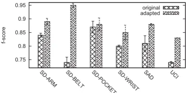
Figure 5: F-score improvement by dynamically and automatically incorporating accelerometer data
In this section, we validate our method by building ac-tivity model with gyroscope data, and dynamically incor-porating accelerometer data to refine the model. 300 weak learners are trained for each activity and thescorethreshold is set to be 0.7 to select examples for retraining, as it is low enough to select sufficient training data and high enough to exclude the noisy examples. We do not perform the iterative process to select the examples and retrain the model, as we found that additional iterations do not provide significant accuracy improvement according to our experiments. On the other hand, repeatedly retraining the model is expensive. For all the experiments, we compare the recognition perfor-mance in terms off-score(f−score=2∗precision∗recall
precision+recall ).
In Figure 5, we can see that, our method (adapted) can improve the recognition accuracy to some extent across the datasets, especially for the dataset that the user fixes the smartphone on the belt. Because it is difficult to distin-guish standing and sitting with gyroscope when the device is put on the belt. However, as belief propagation is able to correct most of the uncertainties, and then the retraining examples would help to refine the initial model. Further-more, the f-score improvement in SD-POCKET setting is marginal. When debugging system, we found that only one weak learner is trained to classify the activitySitting, that means the weak learner overfits the retraining dataset and is unable to classifySittingduring prediction stage if the ac-tivity presents variance. However, when we lower thescore threshold and collect more examples for retraining, the f-score achieves 0.94.
In order to confirm the usefulness of extra features, we look deep into our system and count the proportion of weak learners that are trained on the new features during the re-training process. Since AdaBoost is able to automatically select the weak learner that has the minimum weight er-ror rate in each iteration, the more that the weak learners are trained on the new features, the more discriminative the new features are. As is presented in Figure 6, for most of the dataset the proportions of weak learners trained on new features are more than 50%. From the figure we can see that dataset SD-BELT and SD-POCKET have the propor-tions of 62% and 38% respectively. The underlying reason is that, for the dataset SD-BELT the accelerometer features can better distinguish standing and sitting, and then during the retraining process, more weak learners are trained on the accelerometer data. While in SD-POCKET dataset, the retraining process terminates unexpectedly early for activity
Sitting, and fewer weak learners are trained on the
0.35 0.4 0.45 0.5 0.55 0.6 0.65
SD-ARM SD-BELT SD-POCKET SD-WRIST SAD UCI
proportion of weak learners
Figure 6: Proportion of weak learners trained on new features during the retraining process across the datasets.
5.4
Role of belief propagation
In this subsection, we will examine the role that belief propagation plays in our system. For comparison, we do not perform belief propagation on the intermediate predictions of AdaBoost and choose the most confident examples for retraining, referred to asnoBelief. We also compare with the setting without belief propagation and not considering the extra features (acceleration features), referred to asnoExtra. Therefore,noExtrais exactly the traditional semi-supervised learning that selects the most confident examples to adapt the model, whilenoBelief still considers the incorporation of extra features.
The configurations for these two methods are the same as ours except that the confidence threshold is set to be 0.7 to select examples for retraining. The result is presented in Figure 7, from which we can see that for most of the datasets,noBelief andnoExtra provide marginal f-score im-provement. In some case,noExtra even experiences perfor-mance loss. The reasons are two-fold. On the one hand, high-confidence examples are usually less informative and make less contribution to the f-score improvement. On the other hand, it is difficult to set a universal confidence thresh-old for all datasets. For example, in the dataset SAD, the ac-tivitySittingis frequently classified with a confidence lower than 0.7 (the confidence threshold). Due to the enforcement of retraining data balance, insufficient data of sitting results in a small amount of retraining dataset and hence, less con-tribution in f-score improvement. While in the dataset SD-WRIST, a confidence threshold of 0.7 introduces the noisy examples and has a negative impact on the recognition per-formance.
An exception is found in the dataset SD-POCKET, in which the noBelief achieves the f-score as high as 0.93, as gyroscope performs better than accelerometer in pocket po-sition, confirmed by [19]. Therefore, initial model with gyro-scope is able to correctly recognize most of the activities with high confidence, and provides true labels for the retraining with the combination of accelerometer and gyroscope data, hence the resulting model can then significantly improve the recognition performance. As discussed in the previous sub-section, our method is able to obtain 0.94 in f-score when we lower thescorethreshold.
It should be noted that for most of the datasets (except UCI), traditional semi-supervised method (noExtra) does not provide performance improvement. However, it does not necessarily mean the contradiction between our experiments and previous work [21]. In our cases, the recognition perfor-mance is limited by the discriminative power of the features
0.7 0.75 0.8 0.85 0.9 0.95
SD-ARM SD-BELT SD-POCKET SD-WRIST SAD UCI
f-score
original noExtra noBelief adapted
Figure 7: Comparison withnoBelief andnoExtra in
terms of f-score.
0.82 0.84 0.86 0.88 0.9 0.92 0.94 0.96 0.98 1
SD-ARM SD-BELT SD-POCKET SD-WRIST SAD UCI
f-score
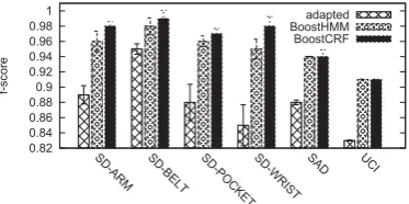
adapted BoostHMM BoostCRF
Figure 8: Combining adapted AdaBoost with HMM and CRF.
rather than the amount of training data, as we build the initial model with sufficient training data, especially for the later two datasets which include activity data from multiple users. The dataset SD-POCKET supports our conclusion. BothnoExtra andnoBelief take the exactly the same data for retraining, but onlynoBelief results in model refinement, due to the fact that it incorporates acceleration features.
To conclude, by incorporating newly discovered features, our method outperforms traditional methods that simply consider the most confident example, and belief propagation followed by examples selection scheme achieves significant improvement in terms of the recognition performance.
5.5
Role of graphical model
In this subsection, we evaluate the recognition perfor-mance by combining AdaBoost with CRF, which is to smooth the accidental predictions given by AdaBoost.
The results are shown in Figure 8, from which we can see that by temporarily smoothing the outliers, the f-score can be improved by 7.9% and 8.2% with BoostHMM and Boost-CRF respectively. The figure also shows that BoostBoost-CRF performs slightly better than BoostHMM, which has been confirmed by previous work [24]. The reason is that, Boost-HMM makes strong assumptions among the variables while BoostCRF have more flexible structures and relationships between connected nodes. Actually, when we look at the re-sults provided by BoostHMM, examples of some continuous activity are still sporadically classified as other classes.
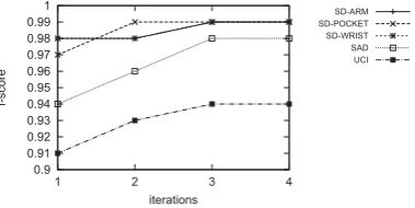
0.9 0.91 0.92 0.93 0.94 0.95 0.96 0.97 0.98 0.99 1
1 2 3 4
f-score
iterations
SD-ARM SD-POCKET SD-WRIST SAD UCI
Figure 9: F-score corresponding to the number of iterations during inference process for BoostCRF.
0.8 0.85 0.9 0.95 1 1.05 1.1
SD-ARM SD-BELT SD-POCKET SD-WRIST SAD
f-score
original adapted
Figure 10: Performance(f-score) improvement by in-corporating magnetometer features, we do not ex-periment on dataset UCI as it does not provide mag-netometer data.
sify the activity with the same dataset, UCI, and obtain the average accuracy of 89.0%. By comparison, we are able to achieve the f-score of 94.0% with BoostCRF. However, we only use the 80 gyroscope features while they build their model on the all of the 561 features.
5.6
Investigation of the usefulness of extra
con-text
In this subsection, we investigate the conditions under which the extra context cannot help with the accuracy im-provement. To this end, we make the following assumptions and perform experiment with the datasets to validate those hypothesises.
1. When the extra context provides less discriminative information compared with existing features.
2. When the initial model is not accurate enough to per-form adaptation.
The basic idea is that extra context, which cannot bet-ter characbet-terize the activities classes or are less discrim-inative than the features upon which the initial model is built, are automatically ignored during the retraining pro-cess. Secondly, if the initial model is not accurate enough, mis-classified examples would be selected for retraining and jeopardise the model. To validate the first assumption, we build the initial model with accelerometer and gyroscope data. During the learning and adaptation stage, the ex-amples contain accelerometer, gyroscope and magnetometer data. As magnetometer data is demonstrated to be overfit-ting [19], magnetic features are less likely to be incorporated during the adaptation stage. The results are illustrated in Figure 10, from which we can see the f-score improvement is insignificant, less than 1% on average. Figure 11 provides a more insightful reason, which shows that only a small
0 0.1 0.2 0.3 0.4 0.5 0.6
SD-ARM SD-BELT SD-POCKET SD-WRIST SAD
proportion of weak learners
Figure 11: Percentage of weak learners that are
trained on magnetometer features during the adap-tation process.
0.4 0.5 0.6 0.7 0.8 0.9
SD-ARM SD-BELT SD-POCKET SD-WRIST SAD
f-score
original adapted
Figure 12: Performance(f-score) decrement with an inaccurate initial model.
tion of weak learners are trained on magnetic features, since they are less discriminative than acceleration features and angular velocity features.
In order to validate the second assumption, we limit the size of initial training dataset, so that the initial model would overfit the dataset and result in an inaccurate classifier. We use 5% of the training data to build the initial model, and present the results in Figure 12. From the figure one can see that, the adapted model would be negatively affected if the initial model is not accurate enough. The underlying reason is that wrongly predicted examples are added to retrain the model. One potential solution to this problem is to be more conservative and increase the weightα3in Eq.(8). However, it is out of the scope of this paper and is left for future work.
6.
CONCLUSION
In this paper, we propose methods to automatically incor-porate dynamically available contexts for activity recogni-tion in dynamic environments. We build the initial activity recognition model with training data, and choose the prof-itable examples to adapt and refine the model. AdaBoost can automatically select the most discriminative features during the adaptation process. We also leverage the tem-poral information of human behaviour to boost the perfor-mance, both in the off-line data analysis and online predic-tions.
personaliza-tion, where general model built with multiple users is then adapted to the specific user at run time. In this light, build-ing the general model is the first step to performbuild-ing person-alization. In the future, we will learn the general model from the data of multiple users, without the constraints that the data has to be labelled or requires the exactly the same data sources.
7.
ACKNOWLEDGMENTS
This work is partially supported by NICTA (National ICT Australia).
8.
REFERENCES
[1] F. Albinali, S. Intille, W. Haskell, and M. Rosenberger. Using wearable activity type detection to improve physical activity energy expenditure estimation. InIn Ubicomp’2010. [2] D. Anguita, A. Ghio, L. Oneto, X. Parra, and J. L.
Reyes-Ortiz. Human activity recognition on smartphones using a multiclass hardware-friendly support vector machine. InAmbient assisted living and home care. 2012.
[3] A. Brajdic and R. Harle. Walk detection and step counting on unconstrained smartphones. In
Ubicomp’2013.
[4] L. Chen, C. D. Nugent, and H. Wang. A
knowledge-driven approach to activity recognition in smart homes.TKDE’2012.
[5] Y. GRANDVALET. Semi-supervised learning by entropy minimization.NIPS’2005.
[6] P. Hevesi, S. Wille, G. Pirkl, N. Wehn, and
P. Lukowicz. Monitoring household activities and user location with a cheap, unobtrusive thermal sensor array. InUbicomp’2014.
[7] P. Hu, J. Indulska, and R. Robinson. An autonomic context management system for pervasive computing. InPerCom’2008.
[8] S. Kang, Y. Lee, and C. Min. Orchestrator: An active resource orchestration framework for mobile context monitoring in sensor-rich mobile environments. In
PerCom’2012.
[9] M. Keally, G. Zhou, G. Xing, J. Wu, and A. Pyles. Pbn: towards practical activity recognition using smartphone-based body sensor networks. In
Sensys’2011.
[10] J. R. Kwapisz, G. M. Weiss, and S. A. Moore. Activity recognition using cell phone accelerometers.
sensorKDD’2011.
[11] O. D. Lara, A. J. P´erez, M. A. Labrador, and J. D. Posada. Centinela: A human activity recognition system based on acceleration and vital sign data.
Pervasive and mobile computing, 2012.
[12] J. Lester, T. Choudhury, N. Kern, G. Borriello, and B. Hannaford. A hybrid discriminative/generative approach for modeling human activities. In
IJCAI’2005.
[13] L. Liao, T. Choudhury, D. Fox, and H. Kautz. Training conditional random fields using virtual evidence boosting. InIJCAI’2007.
[14] G. Luis and O. Amft. mining relations and physical grouping building-embedded sensors and actuator. In
PerCom’2015.
[15] T. Maekawa, Y. Yanagisawa, Y. Kishino, K. Ishiguro, K. Kamei, Y. Sakurai, and T. Okadome. Object-based activity recognition with heterogeneous sensors on wrist. InPervasive’2010.
[16] A. Reiss and D. Stricker. Personalized mobile physical activity recognition. InISWC’2013.
[17] D. Riboni and C. Bettini. Cosar: hybrid reasoning for context-aware activity recognition.Personal and Ubiquitous Computing, 2011.
[18] K. Sankaran, M. Zhu, X. F. Guo, A. L. Ananda, M. C. Chan, and L.-S. Peh. Using mobile phone barometer for low-power transportation context detection. In
Sensys’2014, 2014.
[19] M. Shoaib, H. Scholten, and P. J. Havinga. Towards physical activity recognition using smartphone sensors. InUIC/ATC’2013.
[20] M. Stikic, D. Larlus, and B. Schiele. Multi-graph based semi-supervised learning for activity recognition. InISWC’2009.
[21] M. Stikic, K. Van Laerhoven, and B. Schiele. Exploring semi-supervised and active learning for activity recognition. InISWC’2008.
[22] F.-T. Sun, Y.-T. Yeh, H.-T. Cheng, C. Kuo, and M. Griss. Nonparametric discovery of human routines from sensor data. InPerCom’2014.
[23] E. M. Tapia, T. Choudhury, and M. Philipose. Building reliable activity models using hierarchical shrinkage and mined ontology. InPervasive’2006. [24] T. Van Kasteren, A. Noulas, G. Englebienne, and B. Kr¨ose. Accurate activity recognition in a home setting. InUbicomp’2008.
[25] S. Wang, W. Pentney, A.-M. Popescu, T. Choudhury, and M. Philipose. Common sense based joint training of human activity recognizers. InIJCAI’2007. [26] J. Wen and J. Indulska. Discovering latent structures
for activity recognition in smart environments. In2014 IEEE UIC/ATC/ScalCom Multi-Conference, 2015. [27] J. Wen and M. Zhong. Activity discovering and
modelling with labelled and unlabelled data in smart environments.Expert Systems with Applications, 42(14):5800–5810, 2015.
[28] J. Ye, S. Dobson, and S. McKeever. Situation identification techniques in pervasive computing: A review.Pervasive and mobile computing, 2012. [29] J. S. Yedidia, W. T. Freeman, and Y. Weiss.
Constructing free-energy approximations and
generalized belief propagation algorithms.Information Theory, IEEE Transactions on, 2005.
[30] P. Zappi, C. Lombriser, T. Stiefmeier, E. Farella, D. Roggen, L. Benini, and G. Tr¨oster. Activity recognition from on-body sensors: accuracy-power trade-off by dynamic sensor selection. InEWSN’2008. [31] K. Zhan, S. Faux, and F. Ramos. Multi-scale
conditional random fields for first-person activity recognition. InPerCom’2014.