A Unified NET-MAC-PHY Cross-layer Framework for Performance Evaluation of Multi-hop Ad hoc WLANs

(1)

A Unified NET-MAC-PHY Cross-layer Framework for

Performance Evaluation of Multi-hop Ad hoc WLANs

H

Rachid El-Azouzi

1

, Essaid Sabir

2,∗

, Mohammed Raiss-El-Fenni

1

and Sujit Kumar Samanta

1

1_{LIA-CERI, University of Avignon, 339 chemin des Meinajaries, Agroparc BP 1228, Avignon cedex 9, France.} 2_{RTSE team., GREENTIC/ENSEM, Hassan II University, Route d’El Jadida BP 8118 Oasis, Casablanca, Morocco.}

Abstract

Most of the existing works have been evaluated the performance of 802.11 multihop networks by considering the MAC layer or network layer separately. Knowing the nature of the multi-hop ad hoc networks, many factors in different layers are crucial for study the performance of MANET. In this paper we present a new analytic model for evaluating average end-to-end throughput in IEEE 802.11e multihop wireless networks. In particular, we investigate an intricate interaction among PHY, MAC and Network layers. For instance, we incorporate carrier sense threshold, transmission power, contention window size, retransmissions retry limit, multi rates, routing protocols and network topology together. We build a general cross-layered framework to represent multi-hop ad hoc networks with asymmetric topology and asymmetric traffic. We develop an analytical model to predict throughput of each connection as well as stability of forwarding queues at intermediate nodes in saturated networks. To the best of our knowledge, it seems that our work is the first wherein general topology and asymmetric parameters setup are considered in PHY/MAC/Network layers. Performance of such a system is also evaluated through simulation. We show that performance measures of the MAC layer are affected by the traffic intensity of flows to be forwarded. More precisely, attempt rate and collision probability are dependent on traffic flows, topology and routing.

1. Introduction

In next-generation wireless networks, it is expected that the IEEE 802.11 wireless LAN (WLAN) will play an important role and affect the style of people’s daily life. Further, many factors and applications have made the 802.11 wireless LAN networks an attractive commercial field. The low cost of wireless-network interface was the first encouragement to make the network feasible for civilian applications. The distributed nature of the network and the flexibility that provides were the basis of many interesting applications that do not really need maintenance and reconfiguration.

There are lot of interests in modeling the behavior of the IEEE 802.11 DCF (Distributed Coordination Function) and studying its performances for both architectures: the WLAN networks and multi-hop wireless networks. A medium access control protocol has a large impact on the achievable network throughput and stability for wireless ad hoc networks. So far, the ad hoc mode of the IEEE 802.11 standard

∗

Corresponding [email protected]

has been used as the MAC protocols for MANETs. This protocol is based on the CSMA/CA mechanism in DCF. Over the last decade, there has been a tremendous wave of interest in the study of cooperation in wireless networks, more precisely in wireless ad hoc networks. For instance, the interest has been growing since the publication of famous article of Bianchi [5]. In ad hoc networking context, each neighbor node could assist in the ongoing transmission by exploiting the broadcast nature of the wireless medium. Unfortunately, almost all these studies have been focused on MAC layer without taking into account routing and cooperation level of nodes in ad-hoc networks, see e.g. [1–4,10,14– 16]. In multi-hop ad hoc networks, the majority of efforts are concentrated on extending Bianchi’s model in saturated networks. Now, problem of hidden terminals and channel asymmetry are still real issues for multi-hop ad-hoc networks. Yang et al. [16] proposed an extension of Bianchi’s model [5] and Kumar et al. [8] for multi-hop context under symmetric scenario. They studied the impact of carrier sensing range and the transmission power on the sender throughput. The PHY/MAC impact is clearly presented. Basel et al. [1]

1

Research

Article

EAI Endorsed Transaction

s

on

Mobile

Communications

and

Applications

Receivedon 29 March 2014;acceptedon 14 May 2014;publishedon 24 September 2014

Keywords: Ad hoc network, Performance Evaluation, Cross-layer architecture, Fixed point, Coupled systems.

Copyright © 2014 R. El-Azouzi et al., licensed to ICST. This is an open access article distributed under the terms of the Creative Commons Attribution license (http://creativecommons.org/licenses/by/3.0/), which permits unlimiteduse,distributionandreproductioninanymediumsolongastheoriginalworkisproperlycited.

doi:10.4108/mca.1.4.e6

EAI

for InnovationEuropean Alliance

EAI Endorsed Transactions

(2)

have also interested in tuning the transmission power relatively to the carrier sense threshold. They offered a detailed comparison performance between the two-way handshake and the four-two-way handshake. A three dimensional Markov chain is proposed in [12] to derive the saturation throughput of the IEEE 802.11 DCF. The collision probability is now a function of the distance between the sender and its receiver. The unsaturated node state and the channel state are introduced in [2]. A performance analysis is performed for a single-hop case and a multi-hop case considering that a node can carry different traffic loads. Medepalli et al. [10] proposed an interesting framework model for analyzing throughput, delay and fairness characteristics of IEEE 802.11 DCF multi-hop networks. The applicability of the model in terms of network design is also presented.

Recently, Zhu et al. [17] proposed two cooperative energy efficient algorithms to control the network topology. The authors addressed the problem of inefficient routes that occurs when maintaining the network connectivity, minimizing the transmission power of each node but ignoring the energy-efficiency of paths in constructed topologies. An ordinal potential game formulation is proposed by Chu et al. [19]. They proposed a cooperative approach to determine the transmission power for each node so that it can periodically adapt to the remaining energy on the nodes within its neighborhood. Existence of Nash equilibrium for the game is shown and an algorithm which achieves such equilibrium is proposed. The authors also shown, by simulation, that their algorithm is able to improve the lifetime of a wireless sensor network by more than 50% compared to the best previously-known algorithm. Li et al. [18] studied the throughput of a type of heterogeneous networks consisting of a primary network of sizenand a cognitive radio ad hoc network of size m. The authors shown that the individual throughput of a primary user scales is Θ1/√n with no performance loss due to scaling law. The same result apply for cognitive/secondary users, i.e., the individual throughput scales isΘ1/√m.

Our major goal in this paper, is to build a complete framework to analyze multi-hop ad hoc networks under general and realistic considerations. We present a probabilistic but rigorous model incorporating jointly Network, MAC and PHY layers in a simple cross-layered architecture in a saturated network. This cross-layered architecture has a potential synergy of information exchange among different layers, instead of the standard OSI non-communicating layers. Without any restriction on the network topology, our model is built and valid for any ad hoc network topology under saturation condition. Note that under asymmetry

scenario, nodes do not have the same channel perception. Thus, the attempt rate may not always describe the real channel access activity. Moreover, our model is extended to the IEEE 802.11e1 which provides differentiated channel access (differentiated priority/QoS) to packets by allowing different rates and different back-offparameters. In order to handle QoS, several traffic classes are also supported. We also allow that each traffic/stream may have different retry limits after which the packet is dropped. By analyzing the model, we find that the performance measures of MAC layer may be drastically affected by the routing policy and the traffic intensity of crossing flows. Henceforth, the attempt rate and collision probability are dependent on the traffic flows, topology and routing. From analytical result and as confirmed by simulation, the end-to-end throughput is independent of cooperation level when all forwarding queues are stabled. Hence there is no throughput-delay tradeoff that can be obtained by changing the forwarding probabilities. A real tradeoff is caused by the maximum number of attempts or power control. Indeed, the throughput is ameliorated when reattempting many times on a path, while the service rate on a forwarding queue is slowed down causing low stability region and delay will be increased. A direct application of our work is to find new distributed schemes for channel access and routing that work near optimal stability region of the network. The structure of the paper is as follows : We formulate the problem in Section2. Then we derive the expression of end-to-end throughput and stability that determines traffic intensities in the whole network in Section3. We illustrate our results by some numerical examples in Section4and conclude the paper in Section5.

2. Problem formulation

2.1. Overview on IEEE 802.11 DCF/EDCF

The distributed coordination function (DCF) of the IEEE 802.11 is based on the CSMA/CA protocol in which a node starts by sensing the channel before attempting any packet. Then, if the channel is idle it waits for an interval of time, called the Distributed Inter-Frame Space (DIFS), before transmission. But, if the channel is sensed busy the node defers its transmission and waits for an idle channel. In addition, to reduce collisions of simultaneous transmissions, the IEEE 802.11 employs a slotted binary exponential back-offwhere each packet in a given node has to wait for a random number of time slots, called the back-offtime,

1_{We believe that our model could apply for the recent IEEE 802.11n}

and the future standard IEEE 802.11ac by integrating the adaptive coding and modulation scheme and the Multiple Input Multiple Output technique as well.

2

EAI

(3)

before attempting the channel. The back-off time is uniformly chosen from the interval [0, W−_{1], where} W is the contention window that mainly depends on the number of experienced collisions. The contention windowW is dynamic and given byWi = 2iW0, where

irepresents the stage number (usually, it is considered as the current retransmission attempt number) of the packet, and W0 is the initial contention window. The

back-off time is decremented by one slot each time when the channel is sensed idle, whereas freezes if it is sensed busy. Finally, when the data is transmitted, the sender has to wait for an acknowledgement (ACK) that would arrive after an interval of time, called the Short Inter-Frame Space (SIFS). If an ACK is not received, the packet is considered lost and a retransmission has to be scheduled. When the number of retransmissions expires, the packet is definitively dropped. To consider multimedia applications, the IEEE 802.11e uses an enhanced mode of the DCF called the Enhanced DCF (EDCF) which provides differentiated channel access for different flow priorities. The main idea of EDCF is based on differentiating the back-off parameters of different flows. Thus, priorities can be distinguished different initial contention window, different back-off multiplier or different inter-frame space. An Arbitration IFS (AIFS) is used instead of DIFS. The AIFS can take at least a value of DIFS, and, a high priority flow needs to wait only for DIFS before transmission to the channel. Whereas a low priority flow waits for an AIFS greater than DIFS. In the next paragraph, we used a generalized model of the back-offmechanism.

2.2. Problem modeling and cross-layer architecture

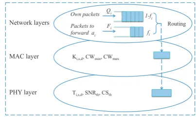
The network layer of each nodei handles two queues, see Fig. 1. The forwarding queue Fi carries packets originated from some source nodes and destined to some given destinations. The second one is Qi which carries own packets of nodeiitself. We assume that the two queues have an infinite storage capacity. Packets are served with a first in first served fashion. When

Fi is not empty, the node chooses to send a packet from Fi with a probability fi, and it chooses to send fromQi with probability 1−fi. When nodeidecides to transmit from the queueQi, it sends a packet destined to node d,d,i, with probabilitypi,d. This parameter characterizes somehow the QoS (Quality of Service) required by initiated service from upper layers. We consider that each node has always packets to be sent from queue Qi, whereas Fi maybe empty. When Fi is empty, the nodeichooses to send a packet from the non empty queueQi with probability 1. Consequently, the network is considered saturated and mainly depends on the channel access mechanism. In ad hoc networks, each node behaves as a router. At each time, it has a packet to be sent to a given destination and starts by finding

the next hop neighbor where to transmit the packet. Clearly, each node must carry routing information before sending the packet. Proactive routing protocols such as the Optimized Link State Routing construct and maintain a routing table that carries routes to all nodes of the network. To do so, it has to send periodically some control packets. These type of protocols correspond well with our model, especially sinceQi is non-empty. Here, nodes form a static network where routes between any sourcesand destinationdare invariant. To consider routing in our model, we denote the set of nodes between a source s and destination d (s and d not included) byRs,d. Each node in our model can handle many connections on different paths. The traffic flow leaving a nodeiis determined by the channel allocation using IEEE 802.11 EDCF. However, differentiating the flow leaving Fi and the flow leaving Qi, allows us to determine the load and the intensity of traffic crossing

Fi. We denote here the probability that the forwarding queue Fi is non-empty byπi. Similarly, we denote the probability that a packet of the path Rs,d is chosen at the beginning of a transmission cycle2 _by _π

i,s,d. This quantity is exactly the fraction of traffic related to the path Rs,d crossing Fi, thus πi =Ps,d:i,sπi,s,d. Next we

analyze each layer separately and show how coupled they are and derive the metrics of interest.

Network layers

MAC layer

PHY layer

Own packets _1-f

i

fi

Ki,s,d, CWmin, CWmax Qi

Fi

Packets to forward ai

Ti,s,d, SNRth, CSth

Routing

Figure 1. Interaction between NET, MAC and PHY layers.

Attempting the channel begins by choosing the queue from which a packet must be selected. Then, this packet is moved from the corresponding queue at the network layer to the MAC layer where it will be transmitted according to the IEEE 802.11 DCF protocol. In this manner, when a packet is in the MAC layer, it is attempted until it is removed from the node.

Accumulative Interference and virtual node : During

a communication between a sender node i and a

receiver nodej in a given path fromstod (where the

2_{A cycle is defined as the number of slots needed to transmit a single}

packet until its success or drop. It is formed by the four channel events seen by a sender. For instance : idle slots, busy slots, transmissions with collisions and/or a success.

3

EAI

(4)

source node of a connection is s and the destination node is d), the node i transmits to j with a power

Ti,s,d. The received power on j can be related to the transmitted one by the propagation relation Ti,s,d· hi,j, where hi,j is the channel gain experienced by j on the link (i, j). In order to decode the received signal correctly, Ti,s,d·hi,j should exceeds the receiver sensitivity denoted by RXth, i.e., Ti,s,d·hi,j ≥RXth. Under symmetry assumption and no accumulative effect of concurrent transmissions, the carrier sense range forms a perfect circle with radiusr1. Even when

considering accumulative interference, the carrier sense can be reasonably approached by a circle with radius

r2≥r1.

Definition 1.The group Z_{, composed of nodes that cannot}

be heard individually by a senderibut their accumulative signal may jam the signal of interest, is called a virtual node. This way, the virtual nodeZ_{is equivalent to a}_fictive

nodebeing in the carrier sense range of senderi.

We can then formulate the carrier sense set of a nodei

by the following expression

CSi =

            

Z_:∀_{s, d, k}0 ∈ Z_,

P

k∈Z

Tk,s,d·hk,i ≥CSth

P

k∈Z\_k0Tk,s,d

·_h_k,i _{< CS}_th

            

, (1)

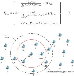
whereCSth is the carrier sense threshold. One can see CSi as the set of virtual nodes that may be heard by sender i when it is sensing the channel in order to transmit on the path Rs,d. In other words, CSi is the set of all real nodes (if they are neighbors of i) and virtual nodes (due to accumulative interferences) that may interfere with nodei. Now, we defineHi,s,d as the set of nodes that may sense the channel busy when node

iis transmitting on the pathRs,d. Then

Hi,s,d ={k:Ti,s,d·hi,k ≥CSth,∀s, d}. (2)

For sake of clarity, we are restricted in our formulation to the case of single transmission power. However, our model can be straightforward used for studying power control from nodes individual point of views. An interesting feature is that when the transmission power level is the same for all nodes and accumulative interferences are neglected, CSi =Hi,s,d. The receiver ji,s,d can correctly decode the signal from sender node i if the Signal to Interference Ratio (SIR) exceeds a certain thresholdSIRth. Let the thermal noise variance, experienced on the pathRs,d, be denoted byNi,s,d, then

SIRji,s,d =

Ti,s,d·hi,j

P

k,i

Tk,s0

,d0·h

k,j+Ni,s,d

≥_SIR_th_, ∀_{s, d, s}0_{, d}0_.

(3) We define now the interference set of a receiver ji,s,d on a path Rs,d, denoted by Tji,s,d, as the collection of

its virtual nodes, i.e., all combination of nodes whose accumulative signal may cause collisions at ji,s,d. For instance, the virtual node Z _{is in the interference set}

of node ji,s,d iff the received signal from node i is completely jammed when nodes in Z_{are transmitting}

all together. The interference set of node j is then written as

T_j

i,s,d =                         

Z_:

T_i,s,d·h_i,j P

z∈Z

Tz,s0,d0·hz,j+Ni,s,d < SIRth,

Ti,s,d·hi,j P

z∈Z\_z0

Tz,s0,d0·hz,j+Ni,s,d

≥_SIR_th_,

∀_z0_{, s}0_{, d}0_{, z}0_,_{i, s}0_,_{s, d}0_,_d.

                        

(4)

Figure 2. The plot shows the transmission range of node iand the set of real nodes Hi,s,d that can hear i when transmitting

to node ji,s,d. The carrier sense CSi of node i and the

interference set T_j

i,s,d are not plotted because they depend

on transmit powers of all nodes in the network as well as the topology and scale of the network. For instance Hi,s,d = {{_s}_,{_j_i,s,d}_,{₆}_,{₁₀}_,{₁₁}_,{₁₂}_,{₁₃}_,{₁₄}_,{₇_,₈_,₉}_,{_d,₄}_, {₁_,₅_,₇_,₈}_,· · · }

Node i

Time Node 8

Node 7 Node 5 Node 6

Success Collision Concurrent transmissions

Figure 3. Effect of accumulative interferences on transmission of nodeito node j

Fig. 2 shows explicitly two different areas that need to be considered when a couple of nodes

4

EAI

(5)

are communicating. Here, we distinguish (i) the transmission area where two nodes can send and receive packets mutually, (ii) the set of nodes that may hear ongoing transmissions of nodei, and (iii) implicitly the carrier sense area where two nodes may hear each other but cannot decode the transmitted data. In Fig.3, we have situated the communication ofiandjon the path

Rs,d. Thus, we can integrate the impact of the routing in the model. Fig.3 illustrates the effect of accumulative interference on the transmission cycles of node i. For illustrative purpose, we consider the following virtual nodes :{₆}_and{₅_,₇_,₈}_{. Node 6 is a neighbor of receiver} j which causes collision whenever they both (nodes

i and 6) are transmitting simultaneously. Whereas a failure may only occur when virtual nodes{₅_,₇_,₈}_are

all transmitting altogether with senderi.

Each node uses the IEEE 802.11 DCF to access the channel and each one can use different back-off parameters. Let Ki,s,d be the maximum number of transmissions allowed by a node i per packet on the path Rs,d. Then after Ki,s,d transmissions the packet is dropped. Also let pi be the back-off multiplier of a given node i. The maximum stage number of node i

is obtained from Wm,i =p mi

i W0,i, where Wm,i andW0,i are, respectively, the maximum and initial contention window for nodei. IfKi,s,d < mithenmitakes the value

ofKi,s,d, otherwisemi =logp_i

_W m,i W0,i

. Using a contention window Wk,i for stage k of node i, the average back-off time for this stage isbk,i. Remark that the back-off parameters of different nodes may be different. Then, the system of nodes are nonhomogeneous as defined by [11].

We consider the modeling problem of the IEEE 802.11 using the perspective of a sender which consists on the channel activity sensed by a sender, or on the state (success or collision) of its transmitted packet. This will facilitate the problem in the ad hoc environment where nodes have an asymmetric vision of the channel. We start by defining the notion of a virtual time slot and channel activity, then we write the expression of the attempt probability for the asymmetric topology. Consider that time is slotted with a physical slot duration τ. Nodes transmit in the beginning of each slot and the transmission duration depends on the type of the transmitted packet. A data packet has a fixed length and takes P ayload (integer) slots to be transmitted (it includes the header transmission time). While an acknowledgment packet spends ACK slots. In our model we consider the two-way handshaking scheme, but it is easily extended to the four-way handshaking scheme. On one hand, a sender node before transmitting would see the channel either busy or idle. On the other hand, its transmitted packet may encounter a success or a collision. These four states define all the possibilities that a sender may observe.

Therefore, the average time spent in a given state (seen by this sender) will be referred as the virtual slot of this sender. A remarkable feature here is that this virtual time would depend on the receiver, i.e., on the path where the packet is transmitted. In fact, the success or the collision of the transmitted packet is itself a function of the actual receiver interference state. For that, we denote by ∆_i,s,d the virtual slot seen by node i on the path Rs,d that we will derive later on. Considering any asymmetric topology, we will always note the metrics functions of the path chosen for transmission. We recall that when we mention the node

ji,s,d, it will be clear that this is the receiver of nodeion the pathRs,d.

In the steady-state and such as [5], we use the key assumption which states that at each transmission attempt, and regardless of the number of retrans-missions suffered, each packet collides with constant and independent probability. However, collisions may depend only on the receiver channel state. For that we denote by γi,s,d the probability that a transmission of a packet of relay i on the path Rs,d fails due to a corruption of either the data or of its acknowledgment. Thus, (1−_γ_i,s,d_{) is the probability of success on the}

pathRs,d. Henceforth, the attempt probability seen by a sender also depends on the receiver, and the well known formula of [5] can be used in the ad hoc network as confirmed in [16]. However, in the asymmetric network the attempt probability (Pi,s,d) (in a virtual slot) for a nodei will be different for each path Rs,d and can be written as in [8]:

Pi,s,d =

1 +γi,s,d+γi,s,d2 +· · ·+γ Ki,s,d−1 i,s,d

b0,i+γi,s,db1,i+γi,s,d2 b2,i+· · ·+γ Ki,s,d−1

i,s,d bKi,s,d−1,i

,

(5) where bk,i = (pkiW0,i−1)/2. On average, a node i will attempt the channel (for any path Rs,d) with a probability Pi which mainly depends on the traffic and the routing table (here, it is maintained by OLSR protocol). Then

Pi =

X

s,d:i∈_R_s,d

πi,s,dfiPi,s,d+

X

d

(1−_π_i_f_i₎_p_i,d_P_i,i,d_. ₍₆₎

Similarly, the average virtual slot seen by node i is written as

∆i =

X

s,d:i∈_R_s,d

πi,s,dfi∆i,s,d+

X

d

(1−_π_i_f_i₎_p_i,d_∆_i,i,d_. ₍₇₎

Remark 1.Theattempt probability (or attempt rate) must be differentiated from the transmission probability. This refers to the probability that a node transmits on any slot. Therefore, the transmission probability, if found, can characterize the channel allocation per node. In WLAN, it is sufficient to analyze the back-offrate to determine the channel allocation rate.

5

EAI

(6)

Note that 1−_π_i_f_i _{is the probability to find a packet}

from Qi in the MAC layer. It seems important to note that the attempt probability represents the back-off expiration rate. It is the transmission probability in an idle slot (only when the channel is sensed idle). For that, it is convenient to work with MAC protocols that are defined by only an attempt probability, this kind of definition may englobe both slotted Aloha and CSMA type protocols including IEEE 802.11. The problem in ad hoc is that nodes have not the same channel vision (or different back-offparameters) and then the attempt probability may not always describe the real channel access. In [11], the problem of short term unfairness was studied in the context of a WLAN.

Collision probability and virtual slot expressions:

The collision probability of a packet occurs when either the data or the acknowledgment experiences a collision. If we denote byγ_i,s,dD andγ_jA

i,s,d,s,d, respectively,

the collision probability of a data packet and its acknowledgement, then we have

γi,s,d = 1−

1−_γD

i,s,d 1−γ A ji,s,d,s,d

, (8)

The attempt probability of a virtual nodeZ_{is defined}

byPZ =Q_z∈ZPz. Therefore, the virtual slot of a virtual

node ∆Z can be reasonably estimated using the

minimum virtual slot among all nodes inZ_{, i.e.,}_∆_Z ₌

minj∈Z∆_j. Thus the probability that transmitted data

collides with other concurrent transmissions can be written as

γ_i,s,dD = 1− Y k∈_H_i,s,d∩T

ji,s,d

(1−_P_k₎

         

1− X

Z∈T

ji,s,d\Hi,s,d

P

P ayload

∆Z

Z          

.

(9) Indeed, nodes in area Hi,s,d∩ Tji,s,d must be silent at the beginning of node i transmission. While nodes in T_j

i,s,d\Hi,s,d are hidden to i (they constitute the

virtual nodes of i) and needs to be silent during all the data transmission time which is a vulnerable time. The P ayload_∆

j is the normalized vulnerable time. After the beginning of data transmission, nodes inHi,s,d will defer their transmission toEIFS(Extended Inter-Frame Space) duration, which would insure the good reception of the acknowledgment. In practice, acknowledgement are small packets and less vulnerable to collision, for that it is plausible to considerγ_jA

i,s,d,s,d

'_{0. Then, we can}

writeγi,s,d =γ_i,s,dD .

Considering the previously defined four states and from the view of nodei, the network stays in a single state a duration equal to∆_i,s,d. It is given by

∆_i,s,d =P_i,s,dsucc.Tsucc+Pi,s,dcol.Tcol+Piidle.Tidle+P busy

i .Tbusy,(10)

where Tsucc =P ayload+ACK+SIFS+DIFS,

Tcol =P ayload+ACK+DIFS, Tidle=τ, Tbusy =

P ayload+DIFS, P_i,s,dsucc =Pi,s,d(1−γi,s,d), Pi,s,dcol =

Pi,s,dγi,s,d, Piidle=

Q

Z∈_CS_i∪{_i}(1−PZ), and P

busy

i =

(1−_P_i₎P

Z∈_CS_iPZ.

Finally, let us denote the equations (5), (6), (8) and (10) bysystem I. Normally, it is sufficient to solve thesystem I to derive the fixed points of each node. However, by introducing the traffic metric in equations (6) and (7), these equations cannot be solved without knowing the

πi,s,d which is defined as the traffic intensity for each path Rs,d crossing node i. Therefore, in Section3, we proceed in writing the rate balance equations at each node, from whichπi,s,dcan be derived as a function ofPj andγj,s,d, for allj. These rate balance equations give the traffic intensity. The problem resides in the complexity of the systems and in the computational issue.

3. End-to-end throughput and traffic intensity

system

We are interested in this section to derive the end-to-end throughput per connection, function of different layer parameters, including the IEEE 802.11 parameters. It is clear that the average performance of the system is hardly related to the interaction PHY/MAC/NETWORK. We focus on the traffic crossing the forwarding queues, which may be an issue on the buffers’ stability. Now, if the arrival and the service rates of a queue are stationary then, from Loynes’ĂŹs theorem, the queue is stable if the arrival rate is less then the service rate. Usually, the stability region is defined to be the closure of the set of all arrival rates vectors such that the network can be stabilized. Hence if the queueFi is stable, then the departure rate of packets from Fi is equal to the arrival rate into it. This is a simple definition of balance rate in the stability region. We are going to derive this equation for each node iand each connectionRs,d. The system of these equations, for alli andRs,d, will form the traffic intensity system, it will be referred as system II. In sum, we are writing a system that determines πi,s,d for all i and Rs,d. For that, we first derive the average length of a transmission cycle per packet Ci at node i. A cycle length on the path Rs,d is formed by the attempt slots that do not lead to a channel access, to a transmission and retransmissions of the same packet until a success or a drop. A cycle may contain idle periods, busy periods, collision periods or/and at most one successful transmission period. Let the random variable (r.v.) Xi (resp. Yi, Zi and Vi) be the number of idle period (resp. the number of busy period, the number of collision period and the number successful period) in a cycle on the pathRs,d. Hence the

6

EAI

(7)

average length in slots of this cycle is given by

ˆ

Ci,s,d =

Ki,s,d−1 X

k=1 ∞ X

l=0 ∞ X

h=0

l+h+k l

h+k h

× ₍_l.T_idle₊_h.T_busy₊_k.T_col₊_T_succ₎_{.P r}_l,h,k,₁

+

l+h+Ki,s,d−1 l

h+Ki,s,d−1 h

× ₍_l.T_idle₊_h.T_busy₊_K_i,s,d_.T_col₎_{.P r}_l,h,K,₀_, ₍₁₁₎

where P rl,h,k,j = (Piidle)l(P busy

i )h(Pi,s,dcol)k(Pi,s,dsucc)j. When a node transmits to several paths, we need to know the average cycle length. Hence, the average cycle of a node is given by

Ci =

X

s,d:i∈_R_s,d

πi,s,dfiCˆi,s,d+

X

d

(1−_π_i_f_i₎_p_i,d_Cˆ_i,i,d₍₁₂₎_.

To write the departure rate fromFias well as the arrival rate into the queue, let us first consider the following counters :

• Ct,i is the number of cycle of the node i till the tth slot, wheret slots means t physical slots and it is equivalent tot.δseconds withδ= 20µsin the IEEE 802.11.

• C_t,iF (resp. C_t,iQ) is the number of all forwarding cycles(resp.source cycles) of the nodeitill thetth

slot.

• C_t,i,s,dF (resp. C_t,i,s,dQ ) is the number offorwarding cycles (resp. source cycles) corresponding to the pathRs,d of the nodeitill thetthslot.

• Tt,i,s,dis the number of times we found at the first slot of a cycle and at the first position in the queue

Fi a packet for the pathRs,d of the nodeitill the tthslot.

• It,i,s,dis the number of cycles corresponding to the pathRs,d of the nodei, where a cycle is ended by a success of the transmitted packet till thetthslot.

• At,i,s,d is the number of arrival packets to nodei on the pathRs,d.

Departure rate : The departure rate from Fi is the probability that a packet is removed from node i

(forwarding queue) by either a successful transmission or a drop after successiveKi,s,d failures. The departure rate regarding only the packets sent on the pathRs,d is denoted bydi,s,d. Formally, for any nodei,sanddsuch that ps,d >0 and i∈Rs,d, the long term departure rate of packets from nodeion the route fromstodis given by the following theorem:

Theorem 1.The long term departure rate from nodeirelated to pathRs,dis given by

di,s,d = fiπi,s,d

Ci

. (13)

Proof. The long term departure rate of packets from nodeion the route fromstodis

di,s,d = _tlim_→∞ C_t,i,s,dF

t

= lim

t→∞

Tt,i,s,d Ct,i

·C F t,i,s,d Tt,i,s,d

·Ct,i

t . (14)

• limt→∞T_Ct,i,s,d

t,i is the probability that Fi carries a packet to the pathRs,d at the beginning of each cycle. Therefore limt→∞Tt,i,s,d_C

t,i =πi,s,d.

• limt→∞

C_t,i,s,dF

Tt,i,s,d is exactly the probability that a

packet is chosen fromFito be sent whenFicarried a packet to the pathRs,d in the first position and in the beginning of a forwarding cycle. Therefore,

limt→∞

C_t,i,s,dF Tt,i,s,d =fi.

• limt→∞_Ct

t,i is the average length in slots of a cycle of the nodei. Moreover, we have

di,s0

,d0 = πi,s

0

,d0f

i

P

s,d:i∈_R_s,dπi,s,dfiCˆi,s,d+Pd(1−πifi)pi,dCˆi,i,d .

(15) Hence from (12), it is easy to derive the total departure ratedi on all paths:

di =

X

s0_,d0_:_i_∈_R

s0,d0

di,s0

,d0= πifi

Ci

. (16)

Arrival rate and end-to-end throughput :The proba-bility that a packet arrives to the queueFi of the nodei is also called the arrival rate, we denote it byai. When this rate concerns only packets sent on the path Rs,d, we denote it byai,s,d. Formally, for any nodesi,sandd such thatps,d >0 andi∈Rs,d, the long term arrival rate of packets intoFi forRs,d is provided by the following theorem

Theorem 2.The long term arrival rate into node i

forwarding queue, related to pathRs,d, is given by

ai,s,d = (1−πsfs)· ps,d

Cs

· Y

k∈_R_s,i∪_s

1−_γKk,s,d k,s,d

. (17)

7

EAI

(8)

Proof. The long term arrival rate of packets intoFi for Rs,d is

ai,s,d = _tlim_→∞ At,i,s,d

t

= lim

t→∞

C_t,sQ Ct,s

·C Q t,s,s,d

CQt,s ·Ct,s

t ·

It,s,s,d

C_t,s,s,dQ

·At,i,s,d It,s,s,d

.(18)

• limt→∞

C_t,sQ Ct,s = 1

− Ct,sF Ct,s = 1

−_π_s_f_s _is _exactly _the

probability to get a source cycle, i.e., to send a packet from the queueQs.

• limt→∞

C_t,s,s,dQ

CQt,s

is the probability to choose the

path Rs,d to send a packet from Qs. Therefore,

limt→∞

C_t,s,s,dQ

CQ_t,s =ps,d.

• limt→∞C_tt,s = _C1

s.

• limt→∞ It,s,s,d

C_t,s,s,dQ is the probability that a source cycle

on the path Rs,d ends with a success, i.e., the packet sent fromQsis received on the queueFjs,s,d.

Therefore, limt→∞ It,s,s,d

C_t,s,s,dQ = 1 −_γKs,s,d

s,s,d .

• limt→∞

At,i,s,d

It,s,s,d is the probability that a packet

received on the nodejs,s,d is also received on the queueFi of the nodei. For that, this packet needs to be received by all the nodes in the set Rs,i∪s.

Therefore, lim t→∞

At,i,s,d It,s,s,d =

Q

k∈_R_s,i∪_s

.

Consequently, the result of the theorem holds.

End-to-end throughput : The global arrival rate at

Fi is ai =Ps,d:i∈_R_s,dai,s,d. Remark that when the node i is the final destination of a path Rs,d, then ad,s,d represents the end-to-end average throughput of a connection fromstod. Practically,ad,s,d is the number of delivered (to destination) packet per slot. Letρbe the bit rate in bits/s of the wireless network. Therefore, the throughput in bits/s can be written as follows:

thps,d =ad,s,d·P ayload·ρ. (19)

Rate balance equations/traffic intensity system :

Finally, in the steady state if all the queues in the network are stable, then for each i,s and d such that

i∈_R_s,d _{we get} _d_i,s,d ₌_a_i,s,d_{, which is the rate balance}

equation on the path Rs,d. For all i, s and d we get the traffic intensity system: system II. When we sum both the sides of this last system, we get the global rate balance equation:di =ai.

Let yi = 1−πifi and zi,s,d =πi,s,dfi. Thus yi = 1−

P

s,d:i∈_R_s,dz_i,s,d. Then, the rate balance equation can be

written in the following form:

X

d:i∈_R_s,d

zi,s,d =

ys(Ps0_,d0z_i,s0_,d0Cˆ_i,s0_,d0+P

d”yipi,d”Cˆi,i,d”)ws,i (P

s0_,d0z_s,s0

,d0Cˆ

s,s0

,d0+P

d”ysps,d”Cˆs,s,d”)

,

(20) wherews,i =Pd:i∈_R_s,dps,dQk∈_R_s,i∪_s

.

An interesting interpretation and application of equation (20) are the following : (i) zi,s,d and yi (can be considered as the stability region of node i) are independent of the choice of fi. (ii) For some values of fi the forwarding queue of node i will be stable. Regarding Pi, we notice that it can be written as Pi =

P

s,d:i∈_R_s,dzi,s,dPi,s,d+Pdyipi,dPi,i,d. Then it depends on zi,s,d and yi, but it is not affected by fi. A similar deduction is also observed for the energy consumed when sensing the channel or transmitting data. LetEi,s,d be the expression of the energy consumed per cycle by each node on the path Rs,d. Let alsoEis be the energy consumed per (virtual) slot in sensing the channel, and

E_i,s,dtx be the energy consumed per transmission of a single packet on the pathRs,d. Therefore, we can derive Ei,s,d from the average cycle length of equation (11) as follows:

Ei,s,d =

Ki,s,d−1 X

k=1 ∞ X

l=0 ∞ X

h=0

l+h+k l

h+k h

× ₍_l.T_idle_.Es

i +h.Tbusy.Eis+k.Tcol.Ei,s,dtx + Tsucc.Ei,s,dtx ).P rl,h,k,1

+

l+h+Ki,s,d−1 l

h+Ki,s,d−1 h

× ₍_l.T_idle_.Es

i +h.Tbusy.Eis+Ki,s,d.Tcol.Ei,s,dtx ).P rl,h,K,0.

This quantity turns out to be independent of the choice offi. Hence, the node can usefito improve the expected delay without affecting the energy consumption. Note that the value πi,s,dfiEri,s,d represents the energy consumption used by nodeito forward packets to path

Rs,d, whereEri,s,d is the energy spent for transmission of one packet.

Resolving PHY/MAC/NETWORK coupled problems :

As have shown previously, the MAC layer systems of fixed points and the Network layer rate balance systems (non linear systems) could not be resolved separately. Moreover, due to dependance on topology, routing and users’ behaviors, we cannot show analytically existence of a unique solution of the fixed point systems. However, for several scenarios and network topologies, system Iandsystem IIalways provide the same solution as obtained from simulation. We give in algorithm 1 a sketch of the algorithmic way we follow to solve mutually the above systems (including the correlation between layers).

8

EAI

(9)

Algorithm 1 : Joint fixed point and rate balance resolution

Require: π_i,s,d0 =i,s,d, δi,s,d : convergence indicator of pathRs,d

1: foreach sources, relayiand destinationddo

2: while

π_i,s,dt+1−_πt

i,s,d πt

i,s,d

≥_δ_i,s,d _do

3: ComputePi,s,dusing fixed point such as [8]

4: Updateγi,s,d using equation (9)

5: Estimate cycles size using equation (12)

6: Update π_i,s,dt+1 by solving the rate balance system (20) using for example the Gaussian elimination method

7: end while

8: end for

Special Cases :For sure thesystem Iandsystem IIare complicated to solve and computational expensive. For that, special cases are important and would facilitate the analysis of the systems and can be useful and easy to use in numerical results. As we have mentioned previously,Pi,s,dandγi,s,d need to be found jointly with πi,s,d. This is due to the traffic asymmetry. Furthermore, the average cycle length Ci is a function ofπi,s,d. This also complicate the calculation ofπi,s,d, whenPi,s,d and γi,s,d are given. Therefore, two special cases can be distinguished as follows:

• Uniform traffic distribution and symmetric topol-ogy:γi,s,d≡γi andPi,s,d ≡Pi. Also,Ci ≡Cˆi,s,d.

• Uniform traffic distribution and asymmetric topology:γi,s,d ,γiandPi,s,d ,Pi. Also,Ci ,Cˆi,s,d, except the case where the routing at each node chooses the same next hop to route packets for all pathsRs,d.

In these two cases, theSystem Iis independent ofπi,s,d, i.e., System I and system II are decoupled. Therefore, we can find the attempt and collision probabilities in System I, and then calculate the traffic intensity. In addition, thesystem IIbecomes a linear system that can be solved easily. Therefore, thesystem IIcan be written as:

1−_y_i ₌ X

s

ysw¯s,i, (21)

where

¯

ws,i =

X

d:i∈_R_s,d

Psps,dCˆi,s,d

Y

k∈_R_s,i

. (22)

Therefore, we can write it in a matrix form:

y(I+ ¯W) = 1, (23)

where ¯W is anN ×_N _{matrix whose (}_{s, i}₎th_{entry is ¯}_w_s,i

(independent on yi) and y is a N−dimensional row

vector. In addition, system I will be simplified when no hidden nodes are found in the network. This case can happen when the interference area of receiversjis included in the carrier sense area of each senderi, i.e.,

Ij\CSi =∅. This imply thatγi,s,d is independent of the virtual slot∆_i,s,d.

4. Simulation and numerical investigations

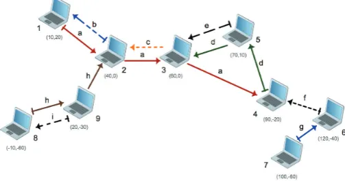
We turn in this section to study a typical example of multi-hop ad hoc networks. We consider an asymmetric network formed by 9 nodes and these nodes are identified using integers from 1 to 9 as shown in Fig.4. We establish 9 connections (or paths) labeled by letters fromatoi. Each node is located by its plane Cartesian coordinates expressed in meters. Apart from this, the main parameters are fixed to the following values :

CWmin= 32,CWmax= 1024,Ki,s,d ≡K = 4,fi ≡f = 0.9 (to insure stability of forwarding queues), Ti,s,d ≡T = 0.1W (∀_{i, s, d}_), _CS_th_{= 0 dBm,} _RX_th _{= 0 dBm,} _SIR_th₌

10 dB (target SIR), ρ= 2 Mbps (bit rate), α = 2 (path loss exponent factor),c= 6 dBi (antenna gain),δ= 20µs

(physical slot duration),DISF= 3δandSIFS =δ.

Model validation : We now present extensive

Figure 4. The multi-hop wireless ad hoc network used for simulation and numerical examples.

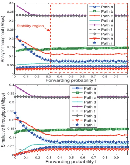
numerical and simulation results to show the accuracy of our model and study the impact of joint PHY, MAC and NETWORK parameters. For this purpose, a discrete time simulator which implements the IEEE 802.11 DCF, integrating the weighted fair queueing over two buffers discussed before, is used to simulate the former network. Each simulation is realized during 106 physical slots, repeated at least 20 times and then averaged to smooth out the fluctuations caused by random number generator of the simulator. We checked the validity of the model by extensively considering different network scenarios and topologies. We depict in Fig. 5 (resp. Fig. 6) the analytic as well as the simulative average load of forwarding queues (resp. average end-to-end delay of considered connections).

9

EAI

(10)

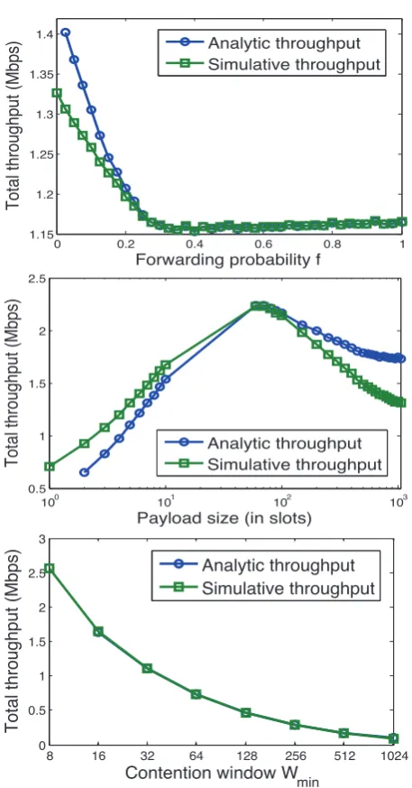
Numerical plots show that analytic model match well with the simulative results, in particular under the stability region which is the main applicability region of our model. With some abuse we refer to the interval of forwarding probability that insure a load strictly less than 1 for all queues, as the stability region. The main difference seen between individual loads is mainly due to the topology asymmetry. Based on Fig. 6, we note that our analytic result says that under the stability condition, the end-to-end throughput does not depend on the choice of the WFQ weight, i.e., on the cooperation level or forwarding probability. Therefore, one can judiciously fine-tune the cooperation level value to decrease the delay when the average throughput is kept almost constant. This mechanism may play a crucial role in delay sensitive traffic support over multi-hop networks. Later, we plot the average throughput versus the normalized payload size (the number of slots required to transmit a packet). We conclude from Fig.7 that an optimal payload size may not exist. Indeed, we note that some specific payload size is providing good performances in term of average throughput over some paths, but may hurt drastically the throughput of other links and then the reachability becomes a real issue. Setting the payload size to a fixed value over the whole network is, in general, unfair and is not suitable for multi-hop networks. However fortunately, existence of locally optimal payload size may exist. This way, it depends strongly on the topology and the local node densities, i.e., the number of neighbors, their respective distances with respect to a tagged node and how they are distributed in the network. Fig. 8shows the variation of average loads of intermediate nodes as a function of the normalized payload. Here,πi is strictly decreasing for all nodes i. This provides an intuition to limit the forwarding queue load (equivalently the delay) by setting the payload size to a high value. Unfortunately, this is unfair and may hurt some connections with more penalizing environment and bad channel state.

Fig.9 plots the average throughput experienced by all established connections when varying the minimum

contention window CWmin. We remark that the

throughput behaves in two different ways according to the topology of the multi-hop network. Indeed, when the node density is low, the throughput is maximized for short backlog duration (connections

e, g and i). Here, nodes take advantage from local node density and tend to transmit more aggressively, having a relatively low collision probability due to low number of competitors. Whereas for other connections, the optimal contention windows size is different from

CWmindefined by the IEEE 802.11 DCF standard. We also note that the contention window tends to increase as the node density becomes high. This latter remark is quite intuitive and due to the fact that the competition

0 0.1 0.2 0.3 0.4 0.5 0.6 0.7 0.8 0.9 1 0

0.2 0.4 0.6 0.8 1

Analytic average load

π i

Forwarding probability f

Node 2 Node 3 Node 5 Node 9

Stability region

0 0.1 0.2 0.3 0.4 0.5 0.6 0.7 0.8 0.9 1

0 0.2 0.4 0.6 0.8 1

Simulative average load

π i

Forwarding probability f

Figure 5. Average forwarding queues load from model versus simulation as function of forwarding probability.

0 0.1 0.2 0.3 0.4 0.5 0.6 0.7 0.8 0.9 1

0 0.05 0.1 0.15 0.2 0.25 0.3 0.35 0.4

Analytic throughput (Mbps)

Forwarding probability f Path a Path b Path c Path d Path e Path f Path g Path h Path i

Stability region

0 0.1 0.2 0.3 0.4 0.5 0.6 0.7 0.8 0.9 1

0 0.05 0.1 0.15 0.2 0.25 0.3 0.35 0.4

Simulative throughput (Mbps)

Forwarding probability f Path a Path b Path c Path d Path e Path f Path g Path h Path i

Figure 6. Average end-to-end throughput from model versus simulation as function of forwarding probability.

10

EAI

(11)

becomes colossal. In terms of queue load (equivalently delay), it is clear that when the contention window increases it implies the increase of queue load and henceforth tagged node may suffer from huge delay.

100 101 102

0 0.5 1 1.5

Payload size (in slots) Path a

Path b Path c Path d Path e Path f Path g Path h Path i

100 101 102

0 0.5 1 1.5

Payload size (in slots) Path a

Figure 7. Average end-to-end throughput from model versus simulation when varying the payload size.

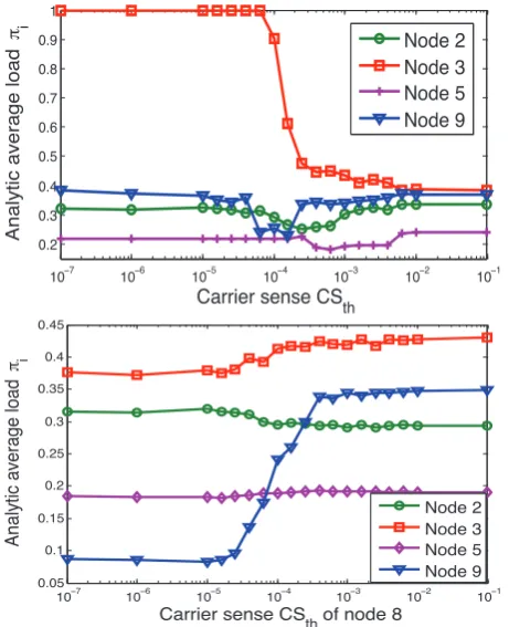
Per path power and carrier sense control : We reconsider here the Spanning tree-based algorithm proposed in [9]. Each node sets its transmission power to a level that allows reaching the farthest neighbor, i.e., the received power is at least equal to the receiver sensitivity. Consequently, this per path power control may improve the spatial reuse. In order to analyze the impact of carrier sense threshold on network performances, we will varyCSth for some tagged node and fix it to the default value, i.e., CSth= 0 dBm. We plot in Fig. 12 the average throughput of all paths when varying the carrier sense threshold of node 3 which is located in a relatively dense subnetwork. We note that the throughput of all connections continues to decrease (in particular connections crossing node 3 or its immediate neighbors) with CSth except connections originated from node 3. Now we analyze the interplay of node 8 (in a low dense subnetwork) carrier sense on network performances. We note that the only negatively impacted connection is connectioni

originated from node 9 (immediate neighbor of node 8). When carrier sense of node 8 is increasing, it becomes more nose-tolerable which implies a more transmission

100 101 102 103

10−20

10−15

10−10

10−5

100

π i

Payload size (in slots) Node 2

Node 3 Node 5 Node 9

100 101 102 103

10−5 10−4 10−3 10−2 10−1 100

π i

Payload size (in slots) Node 2

Node 3 Node 5 Node 9

Figure 8. Average load of forwarding queues from model versus simulation when varying the payload size.

101 102 103

10−4 10−3 10−2 10−1 100

Contention window W_min

Path a Path b Path c Path d Path e Path f Path g Path h Path i

101 102 103

10−3

10−2 10−1 100

Figure 9. Average end-to-end throughput from model versus simulation when varying the minimum contention window.

11

EAI

(12)

8 16 32 64 128 256 512 1024 0

0.2 0.4 0.6 0.8 1

π i

Contention window W

min

8 16 32 64 128 256 512 1024

0 0.2 0.4 0.6 0.8 1

π i

Contention window W

min

Figure 10. Average load of forwarding queues from model versus simulation when varying the minimum contention window.

10−7 10−6 10−5 10−4 10−3 10−2 10−1

0.2 0.3 0.4 0.5 0.6 0.7 0.8 0.9 1

π i

Carrier sense CS

th

10−7 10−6 10−5 10−4 10−3 10−2 10−1

0.05 0.1 0.15 0.2 0.25 0.3 0.35 0.4 0.45

π i

Carrier sense CS_th of node 8

Figure 11. Average load of forwarding queues from model versus simulation for variable carrier sense threshold (in Watt).

10−7 10−6 10−5 10−4 10−3 10−2 10−1

0 0.05 0.1 0.15 0.2 0.25 0.3 0.35

Carrier sense CS

th of node 3 Path a

10−7 10−6 10−5 10−4 10−3 10−2 10−1 0

0.05 0.1 0.15 0.2 0.25 0.3 0.35

Carrier sense CS

th of node 8

Figure 12. End-to-end throughput from model versus simulation for variable carrier sense threshold (in Watt).

10−6 10−4 10−2

1.04 1.06 1.08 1.1 1.12 1.14

Total throughput (Mbps)

Carrier sense CS

th of node 3 Analytic result

Simulative mesure

10−6 10−4 10−2

1.12 1.13 1.14 1.15 1.16 1.17 1.18 1.19 1.2

Carrier sense CS

th of node 8

Analytic result Simulative mesure

Figure 13. End-to-end throughput from model versus simulation for variable carrier sense threshold (in Watt).

12

EAI

(13)

aggressiveness. Which explain the throughput decrease of connection i due to larger backoff duration of node 9 to resolve collision. Thus connections crossing neighbors of node 9 take advantage from the low attempt rate of node 9 to improve their throughput, for instance connectionsa,bandh.

Aggregate throughput :In terms of total capacity and depending on the local node density, the CSC may increase the network throughput. Indeed, when a node in a dense zone fine-tunes its carrier sense threshold, we note existence of a region where the total capacity is maximized. This region correspond to a CSth interval where a tagged node benefits from relatively high throughput and other nodes do not suffer much from this. Whereas, it seems that allowing nodes in low dense parts of the network may cause a throughput decrease due to selfishness of tagged nodes. To sum up, we can say that on one hand, a higher carrier sense threshold encourages more concurrent transmissions but at the cost of more collisions. On the other hand, a lower carrier sense threshold reduces the collision probability but it requires a larger spatial footprint and prevents simultaneous transmissions from occurring, which may result in limiting the system throughput.

Discussion : In contrast to classical systems where all users communicate with an access point and have, in general, the same channel/environment, in ad hoc networks, the main difference is the variable topology and the asymmetric view. A judicious and punctual solution is to auto-configure parameters of the PHY/MAC/NETWORK by the node itself. However unfortunately, this may result in a performance collapse due to users selfishness (similar to prisoners dilemma in game theory). We also suggest to run a MAC/PHY cross-layer control where each node is increasing the transmit power whenever a retransmission is needed. Unfortunately, this power control seems to be unfair since the benefit is strongly depending on the topology. Due to asymmetry, many nodes take benefit from this policy but others may hardly suffer from it. To sum up, under topology asymmetry, the problem is not how to choose parameters such as the network may operate in an optimal way; but the problem is how to define a cooperation level and a trade-off between end-to-end throughput and delay.

Analyzing Fig. 14 where the behavior of the total capacity is depicted as a function of nodes intrinsic parameters (fi, P ayloadi and CWi), we note that the capacity is maximal when a node behaves selfishly, i.e., f = 0. It was shown in our earlier work [7] that a maximum throughput is achieved in the shortest path. A high amount of traffic in the topology of Fig.4is issued from one hop paths, which explains the continuous decrease of the capacity with cooperation levelf. However, the cooperation is crucial to maintain the network connectivity. In view of a game theory and

0 0.2 0.4 0.6 0.8 1

1.15 1.2 1.25 1.3 1.35 1.4

Forwarding probability f Analytic throughput Simulative throughput

100 101 102 103 0.5

1 1.5 2 2.5

Payload size (in slots) Analytic throughput Simulative throughput

8 16 32 64 128 256 512 1024

0 0.5 1 1.5 2 2.5 3

Analytic throughput Simulative throughput

Figure 14. Average cycle size from model versus simulation under different parameters variation.

under node rationality assumption, if a node refuses to forward packets of neighboring nodes then the other may behave similarly. As a result the total capacity may fall down drastically and delay may go to infinity (very large waiting time in intermediate buffers). A challenging but promising concept is then to enable an autonomous location and environment-aware feature. Here, each node may sense the channel, learn the channel state/network topology, decide the best setup, adapt its parameters and reconfigure them till desired QoS is achieved. Nodes can then share their respective information for better environment awareness and less signaling traffic.

13

EAI

(14)

5. Conclusion

In multi-hop ad hoc network, a stack of protocols would interact with each other to accomplish a successful packet transfer. In this context, we have developed a cross-layered model built on the IEEE 802.11e EDCF standard. We studied the effect of forwarding on end-to-end performances for saturated networks. We have discovered that the modeling of the IEEE 802.11 in this context is not yet mature in the literature and to the best of our knowledge, there is no study done which considers jointly the PHY/MAC/NETWORK interaction in a non-uniform traffic and a general network topology. This has led us to build a general framework using the perspective of individual senders. The attempt and collision probabilities are now functions of the traffic intensity, on topology and on routing decision. The fixed point system I is indeed related to the traffic intensitysystem II.

This paper opens many interesting directions to study in future such as power control and delay-based admission control with guaranteed throughput. Moreover, we will deal with the issue of cooperation between nodes in a game theoretical perspective. In addition, our proposal could be easily extended for very high data rate IEEE 802.11n or the future standard IEEE 802.11ac.

References

[1] B. Alawieh, C. Assi, H.T. and Mouftah. Investigation of power-aware IEEE 802.11 performance in multi-hop ad hoc networks. In Proceedings of International Conference on Mobile Ad-hoc and Sensor Networks (MSN), pages 409-420, 2007.

[2] Alizadeh-Shabdiz, F., and Subramaniam, S.: Analytical models for single-hop and multi-hop ad hoc networks. Mob. Netw. Appl., 11(1):75-90, 2006.

[3] Baras, J. S., Tabatabaee, V., Papageorgiou, G., and Rentz, N.: Modelling and optimization for multi-hop wireless networks using fixed point and automatic differentiation. In WiOpt 2008, 6th IEEE International Symposium on Modeling and Optimization in Mobile, Ad Hoc, and Wireless Networks, March 31 - April 4 2008.

[4] Y. Barowski S. Biaz and P. Agrawal. Towards the performance analysis of IEEE 802.11 in multi-hop ad-hoc networks. In Proceedings of IEEE Wireless Communications and Networking Conference (WCNC), pages 100-106, March 2005.

[5] G. Bianchi. Performance analysis of the IEEE 802.11 distributed coordination function. IEEE Journal on Selected Areas in Communications, Volume 18(3), pages 535-547, 2000.

[6] J. Camp, E. Aryafar and E. Knightly. Coupled 802.11 Flows in Urban Channels: Model and Experimental Evaluation. In INFOCOM, San Diego, CA, March 2010. [7] A. Kherani, R. El-Khoury, R. El-Azouzi and E. Altman.

Stability-throughput tradeoff and routing in multi-hop wireless ad-hoc networks. Computer Networks, volume 52(7), pages 1365-1389, 2008.

[8] A. Kumar, E. Altman, D. Miorandi and M. Goyal. New insights from a fixed point analysis of single cell IEEE 802.11WLANs. In INFOCOM, pages 1550-1561, 2005. [9] N. Li, J. C. Hou and L. Sha. Design and analysis of

a MST-based distributed topology control algorithm for wireless ad-hoc networks. IEEE Transactions on Wireless Communications, volume 4(3), pages 1195-1207, 2005. [10] K. Medepalli and F.A.Tobagi. Towards performance

modeling of IEEE 802.11 based wireless networks: A unified framework and its applications. In Proceedings of IEEE INFOCOM, 2006.

[11] V. Ramaiyan, A. Kumar and E. Altman. Fixed point anal-ysis of single cell IEEE 802.11e WLANs: uniqueness, mul-tistability and throughput differentiation. SIGMETRICS Performance Evaluation Review, Volume 33(1), pages 109-120, 2005.

[12] He, J., and Pung H.K.: Performance modelling and evaluation of IEEE 802.11 distributed coordination function in multihop wireless networks. Computer Communications, 29(9):1300-1308, 2006.

[13] T. Sakurai and H.L. Vu. Mac access delay of IEEE 802.11 DCF. IEEE Transactions on Wireless Communications, volume 6(5), pages 1702-1710, 2007.

[14] Vassis, D., and Kormentzas, G.: Performance analysis of IEEE 802.11 ad hoc networks in the presence of hidden terminals. Computer Networks, 51(9):2345-2352, 2007. [15] Vassis, D., and Kormentzas, G.: Performance analysis of

IEEE 802.11 ad hoc networks in the presence of exposed terminals. Ad Hoc Networks, Volume 6(3), pages 474-482, 2008.

[16] Yang, Y., Hou, V., and Kung, L.C.: Modeling the effect of transmit power and physical carrier sense in multi-hop wireless networks. In Proceedings of IEEE INFOCOM, 2007.

[17] Zhu, Y., Huang, M., Chen, S. Wang, Y.: Cooperative energy spanners: Energy-efficient topology control in cooperative ad hoc networks. In Proceedings IEEE of IEEE INFOCOM, Pages 231-235, Shanghai, China, 10-15 April 2011.

[18] Li, C., and Dai, H.: On the Throughput Scaling of Cognitive Radio Ad Hoc Networks. In proceeding of INFOCOM, , Pages 241-245, Shanghai, China, 10-15 April 2011.

[19] Chu X., and Sethu, H.: Cooperative Topology Control with Adaptation for Improved Lifetime in Wireless Ad Hoc Networks. In Proceedings IEEE of IEEE INFOCOM, Pages 262-270, Orlando, Florida, USA, 25-30 March 2012.

14