Mass splitting of heavy-baryons from QCD sum rules

Mass splitting of heavy-baryons from QCD sum rules

R.M. Albuquerque1,a_{, S. Narison}2,b_{, and M. Nielsen}1,c

1 _{Instituto de F´ısica, Universidade de S˜ao Paulo, C.P. 66318, 05389-970 S˜ao Paulo, SP, Brazil}

2 _{Laboratoire de Physique Th´eorique et Astroparticules, CNRS-IN2P3 & Universit´e de Montpellier II, Case 070, Place} Eug`ene Bataillon, 34095 - Montpellier Cedex 05, France.

Abstract. We extract the heavy-baryons mass-splittings due to S U(3) breaking using double ratios of QCD sum rules. We evaluate the masses of the strange-heavy baryonsΞQ,Ξ∗

Q,ΩQandΩ∗Qusing as input the masses of the associated non-strangeΛQ,ΣQandΣQ∗baryons. We notice that the leading term controlling the mass-splittings is the ratio_h¯ss_i/_h¯qq_iof the quark condensate and not the running mass ¯ms. We also predict the hyperfine splittings

Ω∗

Q−ΩQandΞ∗Q−ΞQ.

1 Introduction

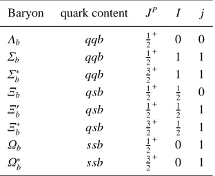
The quantm numbers and quark content of the bottom baryons are shown in Table 1.

Table 1. Properties and valence quark content (q=u or d) of the

bottom baryons. j is the total spin of the light quark pair

Baryon quark content JP _{I j}

Λb qqb 1₂

+

0 0

Σb qqb 12

+

1 1

Σ∗

b qqb

3 2

+

1 1

Ξb qsb 1₂

+ ₁

2 0

Ξ′

b qsb

1 2

+ ₁

2 1

Ξ∗

b qsb

3 2

+ ₁

2 1

Ωb ssb 1₂

+

0 1

Ω∗

b ssb

3 2

+

0 1

TheΛb was the first observed bottom baryon. It was

obsereved at the CERN ISR [1] and was confirmed by sev-eral collaborations. The PDG mass for this state is [2]:

MΛb=(5620.2±1.6) MeV. (1)

Only in 2007, more than 15 years after the observation of Λb, the Σb andΣ_b∗were observed by the CDF

Collabora-tion [3]. They were observed in the decay channelΣ(_b∗)±_→ Λ0_π±_{with the masses given in Table 2.}

Following this discovery, the D0 Collaboration reported the observation of theΞ−

b baryon in the decay channelΞ−b →

a _{e-mail:[email protected]} b _{e-mail:[email protected]} c _{e-mail:[email protected]}

Table 2. Masses of theΣ_b(∗)baryons obsereved by the CDF Col-laboration.

Baryon Mass (MeV)

Σ+

b 5807.8

+2.0 −2.2±1.7

Σ−

b 5815.2±1.0±1.7

Σ∗+

b 5829.0

+1.6+1.7 −1.8−1.8

Σ∗−

b 5836.4±2.0

+1.8 −1.7

J/ψΞ−_{with the mass [4]:}

M_Ξ(D0)

b =(5774±11±15) MeV. (2)

This observation was confirmed by the CDF Collaboration but with a somewhat bigger mass [5]:

M(CDF)_Ξ

b =(5792.9±2.5±1.7) MeV. (3)

The CDF result is in a excelent agreement with the prediction made by Karliner et al. [6], MΞ_b = (5795_± 5) MeV, and also with the predicition from Jenkins [7], MΞb =(5805.7±8.1) MeV.

TheΩ−_b was first observed by the D0 Collaboration in the decay channelΩ−

b →J/ψΩ−with the mass [8]:

M_Ω(D0)

b =(6165±10±13) MeV. (4)

This mass is much higher than expected [9] and is higher than the predicitions from different calculations shown in Table 3. However, a new observation of theΩ−_b, from CDF Collabotation, measured [15]:

M(CDF)_Ω

b =(6054.4±6.8±0.9) MeV, (5)

in a much better agreement with the predicitions in Table 3. The predicition in ref. [14] was done in a QCD sum rule (QCDSR) calculation [16]. Earlier uses of QCDSR [17– 19] for understanding charm and beauty baryons masses

DOI:10.1051/epjconf/201007011

Table 3. Predicition for theΩbbaryon mass from different calcu-lations.

ref. Mass (MeV)

[10] 6052.1_±5.6 [11] 6039.1_±8.3 [12] 6006_±10_±19 [13] 6036_±81 [14] 5820_±230

have been performed in full QCD [20, 21] and in HQET [22], where the results are in quite good agreement with recent experimental findings but with relatively large un-certainties.

Here, we concentrate on the analysis of the heavy baryons mass-splittings due to S U(3) breaking using dou-ble ratios (DR) of QCDSR, which are less sensitive to the exact value and definition of the heavy quark mass and to the QCD continuum contributions than the simple ratios used in the literature to determine the absolute value of heavy baryon masses.

2 QCD Sum rules

The QCDSR is constructed from the two-point correlation function

Π(q)=i

Z

d4xeiq.x_h0_|T [η(x)η(0)]_|0_i. (6)

Lorentz covariance, parity and time reversal imply that the correlator in Eq. (6) has the form

Π(q)= /qΠ1(q2)+Π2(q2). (7) For each invariant functionΠ1andΠ2, a sum rule can be obtained.

The QCD sum rule approach represents an attempt to link the hadron phenomenology with the interactions of quarks and gluons. The method is based on three ingre-dients: a phenomenological description of the correlator, a theoretical description of the same correlator via an oper-ator product expansion (OPE), and a procedure for match-ing these two descriptions and extractmatch-ing the parameters that characterize the hadronic state of interest.

In the phenomenology side, each one of the invariant functions in Eq. (7) can be expressed as a dispersion inte-gral over a physical spectral densityρi:

Π_iphen(q2)=₋

Z

ds ρi(s)

q2_−s+iǫ +· · ·, (8) where the dots represent subtraction terms. The spectral density is described, as usual, as a single sharp pole rep-resenting the lowest resonance plus a smooth continuum representing higher mass states:

ρ1(s)=λ2mBδ(s−m2B)+ρ cont

1 (s), ρ2(s)=λ2δ(s−m2B)+ρ

cont

2 (s), (9)

where λ2 gives the coupling of the current with the low mass hadron of interest and mB denotes the heavy baryon

mass. It is assumed that the continuum contribution to the spectral density,ρcont_i (s) in Eq. (9), vanishes bellow a cer-tain continuum threshold s0. Above this threshold, it is as-sumed to be given by the result obtained with the OPE:

ρcont_i (s)=1

πIm[Πi(s)]Θ(s−s0). (10) In the OPE side, we work at leading order inαs and

consider the contributions of condensates up to dimension six. We keep the terms which are linear in the strange-quark mass ms. After making a Borel transform of both

sides, and transferring the continuum contribution to the OPE side, the sum rules can be written as:

λ2e−m2B/M 2

=

Z s0

m2 Q

ds e−s/M2 1

πIm[Π1(s)], (11)

λ2mBe−m 2 B/M2 ₌

Z s0

m2 Q

ds e−s/M2 1

πIm[Π2(s)], (12) where M2is the sum rule parameter (Borel mass).

An important point of this method is the choice of ap-propriate interpolating current. The lowest dimension gen-eral currents for the spin 1/2 baryons with one heavy quark Q are:

ηΞ_Q =ǫabc h

(qT_aCγ5sb)+b(qTaC sb)γ5

i

Qc,

ηΛ_Q =ηΞ_Q (s_→q) ηΩ_Q =ǫabc

h

(sT_aCγ5Qb)+b(sTaCQb)γ5

i

sc,

ηΣ_Q =ηΩ_Q (s_→q), (13)

where b is an arbitrary mixing parameter.

For the spin 3/2 baryons, we follow Ref. [21] and work with the interpolating currents:

ηµ_Ξ∗ Q

=

r

2 3

h

(qTCγµQ)s+(sTCγµQ)q+(qTCγµs)Q

i

ηµ_Ω∗ Q

= _√1

2η µ Ξ∗

Q

(q_→s)

ηµ_Σ∗ Q

= _√1

2η µ Ξ∗

Q

(s_→q), (14)

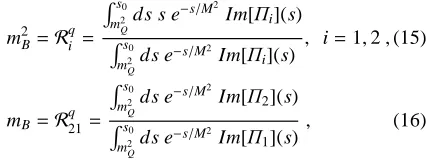
where an anti-symmetrization over colour indices is under-stood. In general one can estimate the baryon masses from the following ratios:

m2_B=Rqi = Rs0

m2 Q

ds s e−s/M2

Im[Πi](s) Rs0

m2 Q

ds e−s/M2

Im[Πi](s)

, i=1,2,(15)

mB=R q

21 =

Rs0

m2 Q

ds e−s/M2Im[Π2](s)

Rs0 m2 Q

ds e−s/M2

Im[Π1](s)

, (16)

-_Π1:

Im[Π1]pert(s)=

(5+2b+5b2)m4_Q 211_π3

1 x2

− 8_x+8x₋x2₋12 ln x

!

,

Im[Π1]ms(s)= 3msm3_Q

28_π3 (1−b 2₎ 2

x

+3₋6x+x2+6 ln x,

Im[Π1]h¯ssi(s)=−

3m_Qh¯ss_i 25_π (1−b

2₎₍₁

−x)2,

Im[Π1]msh¯ssi(s)=

3m_sh¯ss_i 26_π (1+b)

2

1₋x2,

Im[Π1]hG

2_i

(s)=−hg

2_G2

i

212_3π3(1−x)

h

(1+b2) (11x−5)

+2b (7x₋1)], Im[Π1]h¯sgσ.Gsi(s)=h

¯sgσ.Gs_i mQ27π

(1₋b2)13x2₋6x,

Im[Π1]msh¯sgσ.Gsi(s)=−

msh¯sgσ.Gsi

27_3π [(7+22b

+7b2)δ(s₋m2_Q)₋6(1+b)2m 2

Q

s2

      

,

Π₁h¯ssi2(q2)=h¯ssi

2

24 (1−b)

2 1

m2

Q−q2

,

Πmsh¯ssi2

1 (q 2₎₌

−mQmsh¯ssi

2₍₁

−b2₎ 8(m2

Q−q2)2

. (17)

-Π2 :

Im[Π2]pert(s)=

(1₋b)2_m5

Q

29_π3

"

(1₋x) 1 x2

+ 10

x +1

!

+6 1+1

x

!

ln x

#

,

Im[Π2]ms(s)= 3msm4_Q

28_π3 (1−b 2

) 1 x2

− 6_x+3+2x₋6 ln x

!

,

Im[Π2]h¯ssi(s)=− 3m2

Qh¯ss_i 25_π (1−b

2_{)x 1}

−1_x !2

,

Im[Π2]msh¯ssi(s)=−

3msmQh¯ssi

25_π (3+2b+3b 2_{) (1}

−x),

Im[Π2]hG

2_i

(s)=₋mQhg

2_G2

i

211_3π3 (1−b) 2₍₁

−x) 5₋2 x

!

,

Im[Π2]h¯sgσ.Gsi(s)=h ¯sgσ.Gs_i

27_π (1−b 2

)(6+x),

Im[Π2]msh¯sgσ.Gsi(s)=

msmQh¯sgσ.Gsi

27_3π

(25+22b

+25b2)δ(s₋m2_Q)₋3(5+6b+5b2)1 s

,

Π₂h¯ssi2(q2)= mQh¯ssi

2

24 (5+2b+5b 2₎ 1

m2

Q−q2

,

Πmsh¯ssi2

2 (q 2₎₌

−msh¯ssi

2₍₁

−b2) 8(m2

Q−q2)       1+

m2

Q

m2

Q−q2       ,

(18) where x=m2

Q/s. The expressions for the spectral densities

for the other currents are given in ref. [23].

3 Results for

Ω

In the numerical analysis of the sum rules for theΩbwe use

the same values used in ref. [14]: ms=(0.10±0.03) GeV,

mb(mb)=(4.24±0.06) GeV,h¯qqi= −(0.23±0.03)3 GeV3, h¯ss_i=0.8_h¯qq_i,_h¯qgσ.Gq_i =m2

0h¯qqiwith m 2

0 =0.8 GeV 2_,

hg2G2_i=0.88 GeV4.

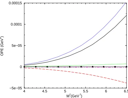
In Fig. 1 we show the contribution of each term in Eq. (17) to the sum rule in Eq. (11), for b =2 and √s0 =

6.5 GeV. We see that we get an excelent OPE convergence. We get a similar OPE convergence for other values of b.

4 4.5 5 5.5 6 6.5

M2(GeV 2) −5e−05

0 5e−05 0.0001 0.00015

OPE (GeV

6 )

Fig. 1. The OPE convergence for the sum rule Eq. (11) forΩb, using √s0 =6.5 GeV and b=2. The dotted, long-dashed, dot-dashed, dotted and solid with squares lines give, respectively, the perturbative, quark condensate, gluon condensate, mixed conden-sate and four-quark condenconden-sate contributions. The solid line gives the total OPE contribution to the sum rule.

However, this is not the case of the sum rule in Eq. (12), since for b = 1, for instance, the perturbative the quark condensate and the gluon condensate contributions van-ishe. For values of b > 1 the perturbative term becames negative. Therefore, we will use only the sum rule in Eq. (11). To obtain the mass of the baryon we use the ratio defined in Eq. (15) with i=1.

In fig. 2 we show the results obtained for mΩb, as a

function of the Borel mass, for different values of b. We see from this figure that we get a reasonable Borel stability, and we get

mΩb =(5.92±0.21) GeV, (19)

4.0 4.5 5.0 5.5 6.0 6.5

M2 (GeV)2

5.00 5.50 6.00 6.50 7.00

MΩ

b

(GeV)

Fig. 2.Ωb mass obtained from Eq. (15) with i = 1 √s0 = 6.5 GeV for b=2 (solid line) and b=₋1 (dashed line).

4 Double ratio sum rules

The uncertainty in Eq. (19) in only due to the values of b and the Borel parameter. Therefore, taking into account the uncertainties due to the values of s0and to the QCD pa-rameters (quark masses and condensates), the uncertainty in Eq. (19) should be even bigger. Besides, there is not a precise criterium to determine the value of the parameter b To try to circumvent these problems, instead of working with the ratios defined in Eqs. (15) and (16), we are going to use the double ratio sum rules (DR) [24]:

r_isd ≡ s

Rs i Rd i

, r₂₁sd ≡R s

21

Rd

21

, (20)

which take directly into account the S U(3) breaking ef-fects. These quantities are less sensitive to the choice of the heavy quark masses and to the value of the continuum threshold than the simple ratios_RiandR21.

For the numerical analysis whe shall introduce the RGI quantities ˆµand ˆmq[25]:

¯ mq(τ)=

ˆ mq

−log√τΛ2/−β1

h¯qq_i(τ)=µˆ3_q−log√τΛ2/−β1

h¯qgσ.Gqi(τ)=µˆ3q

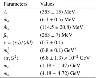
−log√τΛ1/−3β1m2₀, (21) whereβ1=−(1/2)(11−2n/3) is the first coefficient of the βfunction for n flavours, and τ = 1/M2_{. We have used} the quark mass and condensate anomalous dimensions re-viewed in [17]. We use the same QCD parameters as in ref. [23], given in Table 4.

As an example of the DR sum rule we show here the results obtained analysing theΩc(css)/Σc(cqq) and

Ωb(bss)/Σb(bqq) cases.

4.1Ωc(css)/Σc(cdd)

Analysing the Borel mass behavior and continuum thresh-old behavior of of the DR sum rules in Eq. (20), we found

Table 4. QCD input parameters.

Parameters Values

Λ (353_±15) MeV

ˆ

md (6.1±0.5) MeV ˆ

ms (114.5±20.8) MeV ˆ

µd (263±7) MeV

κ_{≡ h}¯ss_i/_hdd¯ _i (0.7_±0.1)

m2

0 (0.8±0.1) GeV 2

hαsG2i (6.8±1.3)×10−2GeV4

mc (1.18∼1.47) GeV

mb (4.18∼4.72) GeV

that r₂₁sddoes not give a result consistent with the one from rsd

i (i = 1,2) and it is also less stable in M

2 _{than the two} others [23]. Therefore, we do not consider r₂₁sd. In Fig. 3 we show the b behavior of rsd

i , i=1,2 for fixed values of M

2

and s0. We see that r₁sdis not stable versus b.

-1 -0.5 0 0.5 1

1 1.02 1.04 1.06 1.08 1.1 1.12 1.14

Fig. 3. The b behavior of the DR sum rules rsd

1 (dashed-dotted line) and rsd

2 (dotted line) for M

2 _{= 1.25 GeV}2

and s0 = 11 GeV2.

The final result from r₂sdis: r_Ωsd

c =1.141±0.039, (22)

which is determined using 6_≤s0 _≤11 GeV2. The sources of the errors come from M2_{, b, s}

0, mc, msandκ. The other

QCD parameters gives negligible errors. Using this result together with the experimental averaged value [2]:

M_Σexp

c =2453.6 MeV, (23)

we arrive at:

M_Ωexp

c =2800±96 MeV, (24)

which is a little higher, but still in agreement (considering the errors) with the experimental result.

4.2Ωb(bss)/Σb(bdd)

the case of the charm, where, only rds

2 survives the diff er-ent tests of stabilities. Here, the s0-behaviour is almost flat from s0 =34 GeV2. The optimal value is taken at M2 =4 GeV2. We obtain:

r_Ωsd

b=1.051±0.012, (25)

with the same sources of errors as before. Using this value together with the experimental averaged value [2]:

Mexp_Σ

b =5811.2 MeV, (26)

one obtain

MΩb =(6108±71) MeV, (27)

which is in a very good agreement with the mean value between the CDF and D0 measurements for MΩ_b.

5 Summary and Conclusions

We have extracted the heavy baryons mass-splittings due to S U(3) breaking using double ratios of the QCD sum rules, which are less sensitive to the heavy quark mass and to the QCD continuum contributions. As a result, we have pro-vided predictions of theΞ(_Q∗)andΩ(_Q∗)masses using the as-sociated non-strange heavy baryons masses from the data. The different results are summarized in Table 5 [23].

Table 5. QSSR predictions of the strange heavy baryon masses in units of MeV from the double ratio sum rules using, as input, the observed masses of the associated non-strange heavy baryons.

Baryons rsd B∗

Q Mass Data

Ξc 1.075±0.021 2458±50 2467.9±0.4

Ωc 1.141±0.039 2800±96 2697.5±2.6

Ξb 1.048±0.015 5888±81 5792.4±3.0

Ωb 1.051±0.012 6108±71 6165.0±13

Ξ∗

c 1.065±0.021 2682±53 2646.1±1.3

Ω∗

c 1.135±0.037 2858±92 2768.3±3.0

Ξ∗

b 1.024±0.008 5973±44 −

Ω∗

b 1.051±0.017 6130±99 −

Combining the predictions for the spin 3/2 baryons with the ones for the spin 1/2 baryons, we give in Table 6 predictions for the hyperfine mass-splittings. These results agree quite well with the data and with some expectations from quark models.

Like in the case of the light baryons [26], it is remark-able to notice that the leading term controlling the mass-splittings is the ratioκ_{≡ h}¯ss_i/_hdd¯ _iof the condensate rather than the running mass ¯ms. This ratio gives, after the choice

of the continuum threshold, the largest errors in rsd

B(∗)_Q.

Table 6. QSSR predictions of the strange heavy baryon hyperfine splittings in units of MeV from the double ratio sum rules using, as input, the predicted values in Table 5

Hyperfine Splittings Observed

MΞ∗_c−MΞc=224±52 179±1

MΩ∗_c−MΩc=58±94 70±3

MΞ∗_b−MΞb=85±63 −

MΩ∗

b−MΩb=22±85 −

References

1. G. Bari et al., Nuovo Cim. A104, (1991) 571; 1787. 2. C. Amsler et al., Phys. Lett. B667, (2008) 1.

3. T. Aaltonen et al., Phys. Rev. Lett. 99 (2007) 202001. 4. V. Abazov et al., Phys. Rev. Lett. 99 (2007) 052001. 5. T. Aaltonen et al., Phys. Rev. Lett. 99 (2007) 052002. 6. M. Karliner, B. Keren-Zur, H.J. Lipkin, J.L. Rosner,

arXiv:0706.2163.

7. E. Jenkins, Phys. Rev. D54 (1996) 4515; Phys. Rev.

D55 (1997) 10. 052001.

8. V. Abazov et al., Phys. Rev. Lett. 101 (2008) 232002. 9. E. Klempt, J.-M. Richard, arXiv:0901.2055.

10. M. Karliner, arXiv:0806.4951.

11. E. Jenkins, Phys. Rev. D77 (2008) 034012.

12. R. Lewis, R.M. Woloshyn, Phys. Rev. D79 (2009) 014502.

13. X. Liu et al., Phys. Rev. D77 (2008) 014031.

14. F.O. Dur˜aes, M. Nielsen, Phys. Lett. B658 (2007) 40. 15. T. Aaltonen et al., Phys. Rev. D80 (2009) 72003. 16. M.A. Shifman, A.I. Vainshtein and V.I. Zakharov,

Nucl. Phys. B147 (1979) 385; 448.

17. For reviews, see e.g.: S. Narison, Cambridge Monogr. Part. Phys. Nucl. Phys. Cosmol. 17 (2004) 1; S. Nari-son, World Sci. Lect. Notes Phys. 26 (1989) 1 ; S. Nar-ison, Acta Phys. Pol. B26 (1995) 687; S. NarNar-ison, Riv. Nuovo Cim. 10(N2) (1987) 1; S. Narison, Phys. Rept.

84 (1982) 263.

18. J.S. Bell and R.A. Bertlmann, Nucl. Phys. B 177 (1981) 218; B187 (1981) 285; R.A. Bertlmann, Acta Phys. Austr. 53 (1981) 305.

19. L.J. Reinders, H. Rubinstein, S. Yazaki, Phys. Rept.

127 (1985) 1.

20. E. Bagan, M. Chabab, H.G. Dosch, S. Narison, Phys. Lett. B278 (1992) 367.

21. E. Bagan, M. Chabab, H.G. Dosch, S. Narison, Phys. Lett. B287 (1992) 176.

22. E. Bagan, M. Chabab, S. Narison, Phys. Lett. B306 (1993) 350.

23. R.M. Albuquerque, S. Narison, M. Nielsen, arXiv:0904.3717.

24. S. Narison, Phys. Lett. B210 (1988) 238; Phys. Lett.

B605 (2005) 319.

25. E.G. Floratos, S. Narison and E. de Rafael, Nucl. Phys.

B155 (1979) 155.