Evaluation of Intensity of Stress Singularity for 3D Dissimilar Material Joints Based on Mesh Free Method (Relationship between Interface Width and Intensity of Stress Singularity)

Published online May 30, 2013 (http://www.sciencepublishinggroup.com/j/ijmea) doi: 10.11648/j.ijmea.20130102.11

Evaluation of intensity of stress singularity for 3d

dissimilar material joints based on mesh free method

(relationship between interface width and intensity of

stress singularity)

T. Kurahashi

1

, A. Ishikawa

2

, H. Koguchi

1 1

Department of Mechanical Engineering, Nagaoka University of Technology, Nagaoka, Niigata 940-2188, Japan

2

Graduate School of Nagaoka University of Technology, Nagaoka, Niigata 940-2188, Japan

Email address:

[email protected] (T. Kurahashi)

To cite this article:

T. Kurahashi, A. Ishikawa, H. Koguchi. Evaluation of Intensity of Stress Singularity for 3D Dissimilar Material Joints Based on Mesh Free Method (Relationship between Interface Width and Intensity of Stress Singularity), International Journal of Mechanical Engineering and Applications. Vol. 1, No. 2, 2013, pp. 28-33. doi: 10.11648/j.ijmea.20130102.11

Abstract:

We present the intensity of stress singularity for 3D dissimilar material joints based on mesh free method. When load is applied to surface of the bonded structure, stress at vertex on interface drastically increases and it appears that this stress singularity occur delamination of the bonded structure. Intensity of stress singularity can be expressed by stress distribution and the intensity of stress singularity. Therefore, it is necessary to obtain the stress distribution precisely. In this study, we focus on the mesh free method for the computation of the stress distribution. When this method is applied to compute stress distribution, incompatible cell can be employed and geometrical data for a target structure can be simply prepared. To confirm the validity of the results of mesh free method, comparison of the intensity of stress singularity between the mesh free and the boundary element methods is carried out.

Keywords:

Stress Analysis by Mesh Free Method, 3D Dissimilar Material Joints, Intensity of Stress Singularity, Order of Singularity

1. Introduction

In this study, evaluation of intensity of singularity for three-dimensional dissimilar material joints based on the mesh free method(MFM) [1] is carried out. If the stress analysis is carried out for 3D dissimilar material joints, the highest value is obtained at vertex on the interface of the dissimilar material joints. This stress value depends on the element size, the value is approached to infinity in case that the element size is gradually small. Therefore, the stress value can’t be applied to the design standard for 3D dissimilar material joints. To solve this problem, we focus on the evaluation by the intensity of singularity.

It is well known that if distance from crack front is r, and stress distribution near crack front is expressed by

0.5 1 /

ij r

σ ∝ . Similarly, stress distribution near edge of interface for dissimilar material joints is also expressed by the relation equation with respect to distance from edge of interface. If the distance from edge of interface is expressed

by r and order of singularity λ is introduced, the relation equation between stress σij and distance r is expressed by

1 / ij rλ

σ ∝ . The order of singularity λ is determined by combination of materials and configuration of edge or vertex.

Here, in case that the order of singularity λ is replaced by 1-p, the stress distribution is written as

1 1

1 / 1 / p p

ij rλ r r

σ _{∝ =} − ₌ − _{. In addition, because the stress}

is expressed as gradient of the displacements u_i , the relationship the displacements and distance r is given

p i

u ∝r by the integration of σij∝rp−1. The parameter p is refer to as the characteristic root, the investigations for the characteristic root of 2D dissimilar material joints is carried out by Bogy [2]. This methodology is analytically approach, it is said that it is difficult this methodology is directly applied to 3D dissimilar material joints.

developed the numerical evaluation method for the singularity based on the finite element procedure. The interpolation function is expressed as the function of rp, and the comparison of the stress intensity factor between the computational and the theoritical solutions was carried out for a cylindrical bar model with circumferential crack. In addition, Pageau et. al. [4] applied this formulation to 3D dissimilar material joints, and the characteristic equation was derived expressed by the characteristic root p. The characteristic root p indicates the eigen value of the characteristic equation, and this value is obtained by eigen value analysis. In the numerical experiments, the characteristic root p at crack front calculated by changing the number of Gauss points and mesh division, and it is reported that there is a tendency the characteristic root converges to an unique value in case that a lot of finite elements are generated, even if the number of Gauss points are changed. Moreover, an application example for models of an anisotoropic three-material junction with a free edge is introduced, the numerical results for the characteristic root is shown.

In addition, Koguchi et. al. evaluate the intensity of singularity for 3D dissimilar material joints based on stress analysis results and the order of singularity λ [5], [6], [7]. The stress analysis is carried out by the boundary element method, and the order of singularity λ is obtained by the characteristic root p that is calculated based on the methodology by Pageau et. al.. Especially, in reference [7], it was clarified that there is a possibility for relationship between delamination force and the intensity of singularity. If numerical analysis for delamination of material is carried out, the remeshing technique is usually introduced. In case that the MFM is applied to the numerical analysis, the remeshing process can be ignored. Though a lot of studies for crack propagation problems using the MFM have been carried out [8], [9], it is difficult to say that researches for evaluation of intensity of singularity using the MFM based on methodology such as the previous studies [5], [6], [7] are carried out enough.

Therefore, the formulation for evaluation of intensity of singularity using the MFM is carried out, and some numerical results and remarks are shown in this paper.

2. Discretization of Elastic Equations by

Mesh Free Method

The equilibrium equation, the strain-displacement relation and the stress-strain relation are written as Equation (1).

(

)

, , ,

1

0, ,

2

ij j ij ui j uj i ij Dijkl kl

σ = ε = + σ = ε (1)

where σij, εij, ui and Dijkl indicate stress and strain

and displacement elastic coefficient matrix. Here, the Equations.(1) are represented as Equation (2).

{ } { } { }

c = 0 , e =

[ ]

B u

{ } { }

, s =

[ ]

D e

{ }

(2)

where

{ }

c ,

{ }

e ,

[ ]

B ,

{ }

u ,

{ }

s and

[ ]

D indicate Equation (3).

{ }

{

, , ,

}

T

xj j yj j zj j

σ σ σ

= c

( j; summation convention)

{ }

T

{

}

x y z xy yz zx

ε ε ε γ γ γ

= e

[ ]

0 0 0

0 0 0

0 0 0

T

x y z

y x z

z y x

_{∂ ∂ ∂} 

 

∂ ∂ ∂

 

 _{∂ ∂ ∂} 

= 

∂ ∂ ∂

 

 _{∂ ∂ ∂} 

 

∂ ∂ ∂

 

B

{ } {

T

}

u v w

=

u

{ }

T

{

}

x y z xy yz zx

σ σ σ τ τ τ

=

s

[ ]

2 0 0 0

2 0 0 0

2 0 0 0

0 0 0 0 0

0 0 0 0 0

0 0 0 0 0

λ µ λ λ

λ λ µ λ

λ λ λ µ

µ µ

µ +

 

 

+

 

 ₊ 

= 

 

 

 

 

 

D (3)

In Equation (3), λ and µ indicate the Lame’s constants, and the constants are written as

(

1 2

)(

1

)

, 2 1

(

)

E E

ν

λ

µ

ν

ν

ν

= =

− + + (4)

Multiplying weighting function u*

( )

x for both sides of equilibrium equation and integrating a domain influence

a

Ω (See Fig. 1.), Equation (5) is obtained.

( )

{

}

{ }

( )

0 a

T

d

Ω Ω =

∫

*

u x c x (5)

Applying the Green theorem to Equation (5), Equation (6) is obtained.

( )

{ }

[ ]

{ }

( )

{ }

( )

{ }

( )

a a

T _T T

d d

Ω Ω= Γ

∫

*

∫

*

u x B s x u x t x (6)

where t indicates traction force, and is written as

{ }

t =

{

tx ty tz

} {

= σxjnj σyjnj σzjnj

}

(7)

( j; summation convention)

displacement-strain relation in Equations (2) to Equation (6) , the Equation (6) is represented as Equation (8).

( )

{ }

[ ] [ ][ ]

{ }

( )

{ }

( )

{ }

( )

a a

T _T T

d d

Ω Ω= Γ

∫

_{u x}* _{B D B u x}

∫

_{u x}* _{t x}

(8)

Figure 1. Domain influence

If the weighting function u* and displacement u at an arbitrary point x is interpolated by each values at referred nodes in domain of influence Ω_a based on the Galerkin procedure, the interpolation function for each values are written as Equations (9) and (10).

( ) ( )

( )

( )

( )

{ }

( )

* * * * *

1 1 2 2 3 3

T

n n

u x =q xu +q xu +q xu⋯+q xu = qx (9)

( ) ( )

1 1 2

( )

2 3

( )

3

( )

{ }

( )

T

n n

ux =q xu+q xu +q xu⋯+q xu = qx (10)

where q indicates shape function, and n indicates number of referred nodes in the domain influence. The shape functions are determined by the moving least square method, and linear basis and quadratic spline functions are employed as the basis function and weighting function. Applying the interpolation functions (Equations (9) and (10)) to the Equation (8), Equation (11) is finally obtained.

[ ]

{ }

{ }

a a

d d

Ω Ω = Γ Γ

∫

Κ u

∫

f (11)

where the left hand side coefficient matrix and the right hand side vector indicate the stiffness matrix and external force vector, and Γ_a indicates the boundary on domain

a

Ω .The Legendre-Gauss formula is employed as the numerical integration for Equation (11). In addition, the penalty function method is employed as treatment of essential boundary condition.

3. Computation of Order of Stress

Singularity

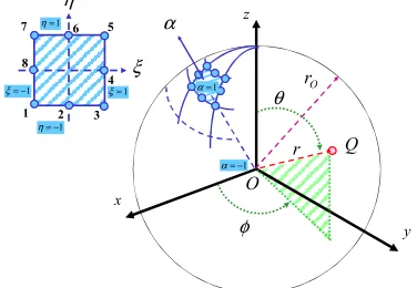
In this section, the derivation of the characteristic equation shown in the reference of Pageau et. al.[4] is simply introduced. In this formulation, the computational region is

defined by spherical configuration whose radius r is r₀, and the spherical coordinate system is introduced (See Fig. 2.). As the final form of the derived equation, the equation on the spherical surface is obtained. Therefore, the surface domain is divided into finite elements, and the computation for the characteristic equation is carried out. In the reference of Pageau et. al.[4], the quadratic isoparametric element is employed as the finite elements.

Figure 2. Computational model and quadratic isoparametric element.

If displacements for each element are expressed by interpolation function shown in Equation (12) and the interpolation function is substituted to equation of the principle of virtual work, a characteristic equation is finally derived as shown in Equation (13).

(

)

0 8

1 , ,

p

r i ri

i

r

u r h u

r θ ϕ

=

 

= 

 

∑

(12)

[ ] [ ] [ ]

(

2

)

{ } { }

p A +p B + C x = 0 (13)

where u_i is expressed by u_i−u_o , and u_i and u_o represent spherical displacements at an arbitrary point in the spherical surface. In addition, h_i indicates the shape function. In the Equation (13), p indicates characteristic

root and vector

{ }

x denotes superposed displacement

vector in entire domain, and matrices

[ ]

A ,

[ ]

B and

[ ]

C represent the coefficient matrices derived by finite element procedure. Detail of this formulation is shown in reference [4]. The characteristic root p is obtained by solving the Equation (13) based on eigen analysis. Relationship between the characteristic root and order of singularity λ is expressed by λ=Re

( )

p −1 . If the parameter λ is

1 λ 0

− < < , it is denoted that stress fields has a stress singularity. On the other hand, if the parameter λis 0<λ, it is denoted that the stress singularity disappears.

4. Numerical Examples

A bonded structure consists of iron and aluminum is employed as the computational model. Scale of computational model is shown in Fig. 3. In this study, the

α

y x

z

O r

Q r 1

=

α

1 − =

α

φ θ

O

1 2 3

4 5 6 7

8

1 = η

1 − = η 1 − =

ξ ξ=1

width “b” of the bonded structure is set 0.25, 0.5, 1.0, 2.0, 4.0, 6.0, 8.0 and 50.0mm, and variation of intensity of stress singularity is investigated. Material properties for each material and total number of evaluation points and cells are shown in Tabs.1 and 2.

Figure 3. Computational model and nodal distribution at vertex on interface

Table 1. Material properties

Material Young’s modulus E

(GPa) Poisson ratio ν

Fe 216.00 0.30

Al 69.69 0.33

Table 2. Total number of evaluation points and cells for each case Width b (mm) Number of evaluation points Number of cells

0.25 _{5,663 4,224}

0.5 5,034 3,618

1.0 6,140 4,506

2.0 5,891 4,280

4.0 _{7,546 5,564}

6.0 _{9,506 7,100}

8.0 11,466 8,636

50.0 8,255 5,976

Computational results by the MFM are shown below. Figs. 4 and 5 show the stress distribution of σ_θθon the interface for the radius direction at ϕ=45deg and θ=90deg and the variation of the stress singularity with respect to model width “b”. Here, the order of singularity λ at vertex is 0.121. In Fig.4, it is seen that stress distribution near vertex decreases with decreasing the width “b”. In addition, it is

found that if the least square approximation for Fig.5 by

1

K_θθ =αbβ , i.e., α and β are fitting coefficients, is carried out, α and β is obtained 7.721 and 0.113, and the value of β is close to the order of stress singularity λ at vertex.

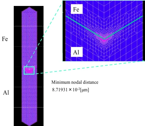
Nextly, the results obtained by the MFM are compared with the results obtained by the boundary element method. The boundary element mesh in case of b=1.0mm is shown in Fig.6. and total number of nodes and elements for each case are shown in Tab.3. The tensile stress same as the case of the MFM is given on the top surface of the bonded structure. Computational results are shown in Figs. 7 and 8. Fig. 7 shows the comparison of stress distribution of σ_θθ in case of the MFM and the BEM. The stress indicates the value on the interface for the radius direction from vertex at ϕ =45deg and θ =90deg. In addition, Fig.8 shows the relationship between the intensity of the stress singularity and the width of the bonded structure obtained by the MFM and the BEM. In Fig.7, it is seen that the stress distribution obtained by the BEM is linearly obtained in semi-logarithmic graph comparing to the results obtained by the MFM. In addition, in Fig.8, it is found that the intensity of the stress singularity obtained by the MFM is close to that obtained by the BEM. However, it is seen that though the gradient of the intensity of the stress singularity with respect to the width of the bonded structure obtained by the MFM is not constant comparing with the result obtained by the BEM. Therefore it appears that some improvements are needed to obtain results with high reliability.

Figure 4. Stress distribution of σ_θθfor radius direction from vertex (φ=45deg θ=90deg)

z

x

y

b[mm]

1.0[mm] 6.0[mm]

Al Fe

σ

z

o 1/8model

Singular point

h[mm]

26

24

22

20

18

16

14

12

S

tr

es

s

σθθ

,M

P

a

3 4 5 6 7 8 9

0.01

2 3

Distance from origin r , mm

Al-Fe interface (θ=90deg, φ=45deg) [mm]

Figure 5. Variation of intensity of stress singularity with respect to model width “b”

Figure 6. Boundary element mesh and magnified figure around vertex (b=1.0mm)

Table 3. Total number of nodes and elements for boundary element model

Width b(mm)

Number of evaluation

point

Number of evaluation

cell

0.5 _{8,930 2,976}

1.0 8,576 2,858

2.0 _{18,554 6,184}

Figure 7. Comparison of stress distribution of σ_θθfor radius direction from vertex in case of MFM and BEM (φ=45deg θ=90deg)

Figure 8. Comparison of intensity of stress singularity with respect to model width “b” in case of MFM and BEM

5. Conclusions

In this paper, we present the intensity of stress singularity based on the stress distribution by the MFM. As the computational model, the bonded structure consists of iron and aluminum is employed. The relationship between width of the structure and the intensity of the stress singularity is investigated by numerical experiments. The width of the bonded structure is varied 0.25, 0.5, 1.0, 2.0, 4.0, 6.0, 8.0, 50.0mm, and linear relationship is consequently obtained between the intensity of the stress singularity and the width of the bonded structure in double-logarithmic graph and if the least square approximation is carried out for the intensity of the stress singularity and the width of interface by

1

K_θθ =αbβ, the value of β is close to the order of stress singularityλ at vertex. In addition, it is found that the results obtained by the MFM are close to the results obtained by the BEM. However, in case that detailed comparison is carried out for the results between the MFM and the BEM, it 7

8 9 10

In

te

n

si

ty

o

f

st

re

ss

s

in

g

u

la

ri

ty

K

1

θθ

,M

P

am

m

0.

12

1

4 6 8

1

2 4 6 8

10

2 4

Width b , mm Al-Fe interface

(θ=90deg, φ=45deg) Curve fiting

Minimum nodal distance 8.71931×10-2[µm]

Al Fe

Al Fe

20

18

16

14

12

S

tr

es

s

σθθ

,M

P

a

3 4 5 6 7 8 9

0.01

2 3

Distance from origin r , mm

Al-Fe interface (θ=90deg) [mm]

MFM_b=2.0 BEM_b=2.0 MFM_b=1.0 BEM_b=1.0 MFM_b=0.5 BEM_b=0.5 Curve fitting

8.0

7.8

7.6

7.4

In

te

n

si

ty

o

f

st

re

ss

s

in

g

u

la

ri

ty

K1

θθ

,M

P

am

m

0.

12

1

5 6 7 8 9

1

2

Width b , mm

is seen that though the gradient of intensity of the stress singularity with respect to the width obtained by the BEM is approximately constant, that obtained by the MFM is not constant. Therefore, it appears that it is necessary to improve the MFM to increase the reliability of the intensity of the stress singularity.

Acknowledgements

This work was supported by Grant-in-Aid for Scientific Research (B) (No. 21360051).

References

[1] T. Belytschko, Y. Y.Lu and L. Gu, “Element-free Galerkin

methods”, Int. J. Numer. Meth. Engrg. 1994; 37(5), pp.229-256.

[2] D. B. Bogy, “Two Edge-Bonded Elastic Wedges on Different Materials and Wedge Angles Under Surface Tractions”, J. Appl. Mech. 1971; 38, pp.377-386.

[3] Y.Yamada, Y.Ezawa and I.Nishiguchi, “Reconsiderations on singularity or crack tip elements”, Int.J.Numer.in Engng.

1979;14: pp.1525-1544.

[4] S.S.Pageau and S.B.Bigger,JR,”Finite element evaluation of free-edge singular stress field in anisotropic materials”, Int.J.Numer.in Engng. 1995;38: pp.2225-2239.

[5] H.Koguchi and T.Taniguchi, “Evaluation of interface strength at the 3D-Corner in Si-resin joint considering residual thermal stresses”, The ASME 2007 InterPACK Conference 2007, 33592.

[6] P.Monchai and H.Koguchi, “Boundary element analysis of the stress field at the singularity lines in three-dimensional bonded joints under thermal loading”, J. Mechanics of Materials and Structures, 2 (1), pp.149-166.

[7] H.Koguchi and M.Nakajima, “Evaluation of the bonding strength at the three-dimensional vertex in silicon-resin joints” The ASME 2009 InterPACK Conference 2009, 89091.

[8] R.D.Borst, M.A.Guierrez, G.N.Wells, J.J.C.Remmers and H.Askes, “Cohesive-zone models, higher-order continuum theories and reliability methods for computational failure analysis”, Int.J.Numer.in Engng. 2004;60: pp.289-315.