An Effective Branch-and-cut algorithm in Order to Solve the Mixed
Integer Bi-level Programming
Arsalan Rahmani a and Majid Yousefikhoshbakht b* aDepartment of Mathematics, University of Kurdistan, Sanandaj, Iran.
bYoung Researchers & Elite Club, Hamedan Branch, Islamic Azad University, Hamedan, Iran. a [email protected]
Abstract: In this paper, a new branch-and-cut algorithm for mixed integer bi-level programming is proposed. For achieving this purpose, a historical perspective of the development of enumeration methods in the field of bi-level linear programming is considered. Then, we present some obstacles for using branch and bound method based on them, and an algorithm is developed to solve for mixed integer bi-level problem. Finally, we use a preference function to determine the choice of branching and specialized cuts in a branch and cut tree. Computational results are reported and compared favorably to those of previous methods and then implications discussed. The results show that not only the proposed algorithm can find high quality solutions for solving a number of the problems, but also it is competitive with other famous published algorithms. Key words: Mixed-integer bi-level programming, Branch and cut method, Fathoming branch.
1. Introduction
An interactive process in which a central unit (leader) coordinates a lower level unit (follower) is called hierarchical organizations. When the follower afforded some level of autonomy, this process becomes more complex to implement, coordinate and optimize. Moreover, in some instances, the objectives of the follower may conflict with those of the leader. In mathematical programming environment, these interactive processes are existed and known as bi-level or multi-level programming. Linear bi-level programming problems (BLPP) generally involve a hierarchy of two optimization problems, in the following form:
1 1 1:maxx 1
P Z =c x d y+
1 1 1
. .
s t A x B y g+ ≤
x X∈
2 2
max
y c x d y+
2 2 2
. .
s t A x B y g+ ≤
y Y∈
1 1 , 2 2 c x d y c x d y+ +
are called upper level and lower level objective function,
1 1 1
A x B y g+ ≤
and
2 2 2
A x B y g+ ≤
are known as upper level and lower level constraints respectively. Upper-level constraints involve variables from both levels. In this paper, a special class of BLPP is considered and its model is supposed to have the following characteristics:
- In the upper level problem, the constraints do not include any variable from the lower level problem.
The most competitive facility location problems lay in this group, in fact decisions about the location of facilities (for the first decision maker (leader)), capacities of facilities, transportations and so on are full free of lower level variables, the lower level variables may take into accounts in upper level’s objective function.
- For any feasible solution of upper-level problem, there is a feasible solution for the lower-level problem.
In the problems, which a level of service is objective, when one company is not able to service a customer, the other company do it. As a result, in this case for any feasible solution of upper-level problem, there is a feasible solution for the lower-level problem.
A special case of this type of problem is discrete competitive facility location problem (Beresnev, 2009). Jeroslow showed that Bi-level programming problems are NP-hard even in the “simplest case”, the linear BLPP (Jeroslow, 1985) while (Hansen et al., 1992) proved that the problem is strong NP-hardness. Regarding to solution approaches, many algorithms were proposed in literature. Gümüş studied global optimization of bi-level programming problems (Gümüş and Floudas, 2005), and proposed a convex relaxation of the inner problem followed by its equivalent representation via necessary and sufficient optimality conditions. The approximated branch and bound global optimal principles presented a branch and bound framework. The first precise global optimization approach for the calculation of the
flexibility test that is bi-level nonlinear optimization model is introduced in (Floudas et al., 1999). Then they demonstrate its applicability to a heat exchanger network problem, a pump and pip problem, a reactor-cooler system and a prototype process flow sheet model. Pistikopoulos introduced methods based on parametric programming to transform the bi-level problem into a family of single level optimization problems which can be solved to global optimality (Pistikopoulos et al., 2007), and presented computational results on several small benchmarks linear-linear, linear-quadratic, quadratic-linear and quadratic-quadratic type problems. Moreover, two new methods for bi-level programming problem are proposed (Gümüş and Floudas, 2005). In the case of bi-level linear programming different algorithms proposed in (Vicente, 2001), (Colson et al., 2005) and (Domínguez and Pistikopoulos, 2010). Dempe considered the case characterized by continuous upper-level variables and integer lower-level variables, and used a cutting-plane approach to approximate the lower-level feasible region (Dempe, 2001). Wen considered the opposite case, where the lower-level problem is a linear program and the upper-level problem is an integer program (Yang, 1990). Linear programming duality employed to derive exact solutions. In The discrete case, Moore developed a basic enumeration scheme to identify feasible solutions (Bard and Moore, 1990). Beside these methods an applicable Lagrangean based algorithm also proposed in (Rahmani A, 2015) and the metaheuristic method using particle swarm optimization method has been used for solving a special class of Bi-level problem (Mirhassani, 2015).
demonstrates a better performance respect to the branch-and bound algorithm (Bard and Moore, 1990; Beresnev and Melnikov, 2014), and branch and cut algorithm (Denegre and Ralphs, 2009). It can be implemented in a straightforward way using existing software. The computational results show the algorithm efficiency in terms of solution quality and running time.
The rest of the paper is as follows. In Section 2, we describe the mathematical models and the challenge of solving the models by generalizing solution methods for single-level mathematical programming problems. In Section 3, we propose a branch-and-cut algorithm for MIBLPs and section 4 illustrates the algorithm via an example and provides some preliminary computational results. Finally, in Section 5, we provide conclusions and directions for future work.
2. Definitions and Notation
Bard and Falk (Bard and Falk, 1982) utilized the following notation and definitions in their work.
BLPP Constraint Region:
( , ) |x y A x B y g A x B y g x X y Y1 1 # 1, 2 2 # 2, ! , !
X=" + + ,
Projection of Ω onto the Leader’s Decision Space:
( )X x X y Y A x B y g A x B y g! |7 ! , 1 1 # 1, 2 2 # 2
X =" + + ,
Follower’s Feasible Region for
x X
∈
Fixed:( )x y Y A x B y g! | 2 2 # 2 X =" + ,
Follower’s Rational Reaction Set for x∈Ω( )X :
( ) { | argmax[ | ( )]}
M x = y Y y! ! y c x d y y2 + 2 !X x
Inducible Region:
( , ) | ( , )x y x y ,y M x( )
R=" !X ! ,
In order to make P1 well posed it is assumed that Ω is non-empty and compact, and for each decision taken by the leader there is some room to move for the follower, or X( )x !Q.
Definition 1: If y M x∈ ( ) then y is said to be optimal with respect to x; such a pair is said to be bi-level feasible.
Definition 2: A point (x*, y*) is said to be an optimal solution to the BLPP if
a) (x*, y*) is bi-level feasible; and,
b) For all feasible pairs (x,y); c1x+d1y≤c1x*+d1y*.
Definition 3: We said (x, y) is valid for a cut (set); if it satisfied in this cut (set).
Definition 4: An inequality defined by (a,b,g) is said valid for set S, if for all pairs( , )x y ∈S; ax+by ≤ g
Bard and Moore postulated several obstacles to the development of algorithms to solve P1 (Bard and Moore, 1990). They established 3 observations for general mixed integer programming problems. Fathoming in normal linear programming scenarios presents problems and follows 3 observations.
Observation1: The solution of the relaxed BLPP does not provide a valid upper bound on the solution of the mixed integer BLPP.
Observation2: Solutions to the relaxed BLPP that are in the inducible region cannot, in general, be fathomed.
Observation3: Not all integer solutions to the relaxed BLPP with some of the follower’s variables restricted can, in general, be fathomed.
In the BLPP, unfortunately, only observation1 can be applied with any degree of confidence.
Observation 2 needs some strong qualification and observation3 must be discarded altogether.
To initialize the cutting plane procedure, first introduce some notations:
With any loss of the generality let all variables are binary, and n the number of binary variables of upper level problem.
k: The order number of a generated node in a branch-and-cut tree:
Jk0 ={j | x
jis a free binary variable, j=1,2,…,n}
Jk+ ={j | x
jis a fixed at 1, j=1,2,…,n}
Jk– ={j | x
3. Branch and Cut Algorithm
One common route with many classes of mathematical programs for achieving global optimality in the branch and bound and branch and cut algorithm, is the development of a bounding strategy. Based on the observations, the bounding, fathoming, and branching procedures employed in traditional LP-based branch-and-bound algorithms is not applicable in a straightforward way. In this section, we use previous works that describe how to overcome these challenges to develop a generalized branch-and-cut algorithm for MIBLP that follows the same basis used in MILP.
3.1. Bounding
Wen in (Yang, 1990) proved the following lemmas:
Lemma 1: Given two linear programming problems:
P2:max Z2=cx P3:max Z3=cx
s.t. Ax ≤ b s.t. Ax ≤ b+θ x ≤ 0 x ≤ 0
Where, θ is a parameter vector. Let Z2* be the optimal objective value of P2 , V2* the dual optimal solution of
P2 , Z3* the optimal objective value of P
3 ; and V3* the dual optimal solution of P3 . Then
Z3* ≤ Z 2* +V2*θ
Proof: see (Yang, 1990)
Lemma 2: The optimal value of the leader’s objective function in the P1 is less than or equal to the optimal objective function value in the following problem P4.
P4:max Z2=c1x+d1y
s.t. A1x+B1y ≤ g1
A2x+B2y ≤ g2
,
x X y Y
∈
∈
Proof: see (Yang, 1990)
Theorem 1: Consider the following problem P5( x ): P5( x ): max Z5=d1y
s.t. A1x+B1y ≤ g1
A2x+B2y ≤ g2
y≥0
Let Z5* be the optimal objective function value for the problem P5 and V5* the optimal dual solution of the problem P5 . Then the following upper bound,Z5U
is established for the leader’s objective function value in problem P1 when x = x is fixed.
0
5 5 ( 5 ) max{( 5 ),0}
k k
U
j j j j
j J j J
Z Z c V a c V a
+
∗ ∗ ∗
∈ ∈
= +
∑
− +∑
−That is Z5U≥d1y*+c1x*
Where aj is the j th column vector of the matrix 1
2
A A
.
Proof: see (Yang, 1990)
Generating Valid Inequalities
There is two more observation, which is related to feasible cuts:
Observation4: If an inequality is valid for set Ω, it is also valid for the main Bi-level problem, i.e. set R
Observation5: Let (x,y) ∈ Ω, but (x,y) is not bi-level feasible (i.e. y∉M(x)), then if one inequality is valid for Ω -{(x,y)}, it is also valid for the main Bi-level problem (R)
Because of the relationship Ω⊆R, Observation4 is derived. So, we can remove fractional solutions which are LP (removal of the lower-level optimality and integrally restrictions) resulting from the R; and based on Observation5 we can separate points from the R that are integer but not bi-level feasible.
the original problem, but we would like to add an inequality to P5 that is valid for P1 and violated by (x, y). The following simple procedure shows how to generate such an inequality.
Let (x,y) be a feasible point in upper and lower levels constraints without integer constraints and S be the set of constraints binding at (x,y) , then following cut is valid for the main Bi-level problem P1.
1
Fx Ey G+ ≤ −
Which i, i, i
i S i S i S
F a E b G g
∈ ∈ ∈
=
∑
=∑
=∑
and ai , bi , gi are the coefficient of x, y and right hand side respectively.
3.2. Branching
The algorithm which delivered by Moore and Bard (Bard and Moore, 1990), is forced to branch after producing an infeasible integer solution but here we are free to employ the well-developed branching strategies used in traditional algorithms for ILP, such as pseudo-cost branching, or the recently introduced reliability branching (Achterberg et al., 2005). A branching technique for bi-level problems is dis-cussed in following paragraph.
Let a solution of P5 be in hand and
0
k
i J∈ i.e. xi be a free variable, From theorem 1, an upper bound is obtainable byZ5U. Now, letZ5U+,Z5U− be the value of
5
U
Z forxi=1or xi=0respectively. The upper bound is Z5U= max {Z5U+ ,Z5U−}. As part of the iterative
pro-cess, the upper bounds have to be checked against the current upper bound on the objective function Z*. If the upper bound on that particular branch is not greater than the current best solution then that branch fathomed. Now we propose the following algorithm to solve the mixed integer bi-level linear program-ming problem.
4. The proposed algorithm
The algorithm depends heavily on the preceding observations, lemmas and theorem. Especially the relaxation of the problem from a two-level problem to a simple MIP, which is easy and quickly solvable compared to solving a complex bi-level linear programming problem. Establishing the relaxed problems is the first priority of the algorithm and is completed in steps 1 and 2. This provides a lower bound for the problem by fixing all leaders’ binary variables to zero, in both the leader’s objective
function and the follower’s objective function. By the way the follower’s objective function does not contain any leader’s binary variables. Therefore, all terms in follower’s objective function related to leader reduce to a constant at the time of optimization and hence will not affect optimum solution. This allows the ignoring of the leader’s variables in the formulation of the follower’s objective function. The algorithm outlined in 7 steps.
Step 1: Initialization
N = 0; k = 0
N is a place-keeper of the current level in the tree, k is the counter for evaluating nodes
0 {1,2,..., }
k
J = n Jk+={}Jk−={}
0, 1,2,...,
j
T = j= n
This indicates that all the leader’s variables are free.
Step 2: Relaxed solution
Let x is the solution related to the kth node. Solve problem P5 with the fixed x and obtains y:P5→( , )x y .
These results inZ5∗, the optimal objective function
value, and V5∗ , the optimal dual solution.
Follower solution: solve follower problem by fixing x and obtain ŷ
If the problem results inZ x y1( , )ˆ ≥Z1∗; then
Z1*=Z1 (x, ŷ ) otherwise Z1∗=Z1∗
Step 3: Branching
Calculate the upper bound of the leader’s objective function from the previous node, (k-1), and xN=0. This denoted asZUN5−. Similarly calculatesZUN5+where
1
N
x = . ZNU5=max"Z ZUN+5, NU5–, and TN=TN+1.
Step 4: Cut generation
Generate the following cuts:
Z1)+f#c x d y1 + 1
1
Which S is the set of constraints binding at( , )x y1 ,
, ,
i i i
i S i S i S
F a E b G g
∈ ∈ ∈
=
∑
=∑
=∑
and ai ,bi ,ci are the
coefficient of x, y and right hand sight respectively.
Step 5: Optimality check
If ZUN5+<Z1∗then set TN=2; go to Step 6.
The next step requires that if the algorithm has arrived at a node at the bottom of the tree (there is no free variable) then it can proceed back up the tree, examining branches and their upper bounds along the way. Each upper bound compared to the current best solution to determine whether the branch fathomed or must be considered further. This described in the next step.
Step 6: Backtracking
If TN=2 then set TN=0, N=N–1.
If N=0 (i.e. we came back to the top of the tree, and all possible nodes are evaluated) go to Step 7. Else, TN=TN+1.
If 1 0
N
x = then the upper boundZUN5+=ZNU5 andx1N=1; ElseZNU5−=ZNU5 andx1N =0; go to Step 4.
Step 7: Termination
Stop algorithm execution and output the solution.
The following simple numerical example illustrates the algorithm. In this example we use the notation P(i,–j), it means that the variable xi is fixed to one, the variable xj is fixed to zero and the other variables are free.
Example 1:
P6: max 15x1+2x2+20x3+10x4+10y1+15y2+20y3+5y4+12y5 max 5y1+3y2 +8y3+4y4+y5
6x1+5x2+10x3+12x4+6y1+3y2+9y3+2y4+2y5≤12 2x1+4x2+13x3+7x4+5y1+y2+3y3+3y4+y5≤19 3x1+8x2+9x3+9x4+10y1+5y2+6y3+4y4+6y5≤15 4x1+3x2+12x3+14x4+4y1+3y2+5y3+y4+6y5≤30 xi, yj ∈ {0,1}
In the initialization phase let x=( , , , )x x x x1 2 3 4 are free and try to solve the following problem where x=0:
7 1 2 3 4 5
1 2 3 4 5
1 2 3 4 5
1 2 3 4 5
1 2 3 4 5 1
2 3 4 5
() : max10 15 20 5 12
6 3 9 2 2 12 (1)
5 3 3 19 (2)
10 5 6 4 6 15 (3)
4 3 5 1 6 30 (4)
0 1, (5)
0 1, (6)
0 1, (7)
0 1, (8)
0 1, (9)
P y y y y y
y y y y y
y y y y y
y y y y y
y y y y y
y y y y y
+ + + +
+ + + + ≤
+ + + + ≤
+ + + + ≤
+ + + + ≤
≤ ≤
≤ ≤
≤ ≤
≤ ≤
≤ ≤
This gives (0,1,0.809,0,0.857) with the objective value 41.487 and dual solution V7*()=(1.143,0,1.619,0,0,3.476,0,0,0) the related optimal solution for the following problem is y=(0,0,1,1,0) with the objective value 25.
The binding constraints of this solution are:
Constraint One:
(6x1+5x2+10x3+12x4+6y1+3y2+9y3+2y4+2y5≤12),
Constraint Three:
(3x1+8x2+9x3+9x4+10y1+5y2+6y3+4y4+6y5≤15) and the constraint Six:
(0≤y2≤1), so, F=(6,5,10,12)+(3,8,9,9), E=(6,3,9,2,2)+(10,5,6,4,6)+(0,1,0,0,0) and G=12+15+1, therefore the binding cut is:
9x1+13x2+19x3+21x4+16y1+9y2+15y3+6y4+8y5≤27 (10)
and the objective cut is:
15x1+2x2+20x3+10x4+10y1+15y2+20y3+5y4+12y5≥26 (11)
The first choice facing the algorithm is processing with x1=0 or x1=1. (Our choice variable is random; one can use an appropriate heuristic to select sequence of variables like greedy algorithms) The choice is made dependent on the relative values of the upper bounds for each branch. In this particular case under examination these values are Z7U−= 41.476
andZ7U+= 44.762. At this point it would be a useful
{}
k
J+= , since all 7
j j
c V a− ∗ ’s are negative excepting
1 7 1 3.286
c V a− ∗ = then
7 = 41.476
U
Z − , and if 1 1 x =
then 0 {2,3,4}
k
J = , Jk+={1} andZ7U+= 44.762.
So, for the first iteration 0 {2,3,4}
k
J = , Jk+={1} and {}
k
J−= is considered.
Using x =(1,0,0,0) the integer linear programming problem Z7, becomes:
7 1 2 3 4 5
1 2 3 4 5
1 2 3 4 5
1 2 3 4 5
1 2 3 4 5
1 2 3 4 5
1 2 3 4 5
(1) : max10 15 20 5 12
6 3 9 2 2 6
5 3 3 17
10 5 6 4 6 12
4 3 5 1 6 26
16 9 15 6 8 17
10 15 20 5 12 11
0 j 1
P y y y y y
y y y y y
y y y y y
y y y y y
y y y y y
y y y y y
y y y y y
y + + + + + + + + ≤ + + + + ≤ + + + + ≤ + + + + ≤ + + + + ≤ − − − − − ≤ − ≤ ≤
This gives (0,1,0.1,1,0) with the objective value 7.8 and dual solutionV7∗(1) (0.8,0,0,0,0,0,0,0.3,0,2.2,0)= ,
the related optimal solution for the follower problem is (0,1,0,1,0) with the objective value 35, so till now
35
Z∗= .
The binding constraints of this solution are one, eights and tenth, so the next cuts are:
6x1+5x2+10x3+12x4+6y1+4y2+9y3+3y4+2y5≤9
15x1+2x2+20x3+10x4+10y1+15y2+20y3+5y4+12y5≥36
Now, if x2=0 then Jk0={3,4} and Jk+={1}, then
5U = 44.762
Z − , and if
2 1
x = then 0 {3,4}
k
J = ,
{1,2}
k
J+= and
7 = 28.09
U
Z + .
So, for the next iteration (k=2) 0 {3,4}
k
J = , Jk+={1}
and Jk−={2} is considered.
Using x =(1,0,0,0) the integer linear programming problem P7(1, 2)− , in the example, now becomes:
7 1 2 3 4 5
1 2 3 4 5
1 2 3 4 5
1 2 3 4 5
1 2 3 4 5
1 2 3 4 5
1 2 3 4 5
(1, 2) : max10 15 20 5 12
6 3 9 2 2 6
5 3 3 17
10 5 6 4 6 12
4 3 5 1 6 26
16 9 15 6 8 3
10 15 20 5 12 21
0 j 1
P y y y y y
y y y y y
y y y y y
y y y y y
y y y y y
y y y y y
y y y y y
y − + + + + + + + + ≤ + + + + ≤ + + + + ≤ + + + + ≤ + + + + ≤ − − − − − ≤ − ≤ ≤
This problem is infeasible and then this branch is fathomated.
The backtracking can now take place. It will examine the node associated with x2=1 and conclude that sinceZ7U+=28.09, is less than the current Z *=35, the
node is fathomated. By examining the other nodes, the following results obtained:
Node k=3:
0 {3,4}
k
J = , Jk+={}, Jk−={1,2}, Z7U+=24.8,
7 41.47
U
Z −= , Z∗=35.
Node k=4:
0 {4}
k
J = , Jk+={}, Jk−={1,2,3}, Z7U+=24.8,
7 41.47
U
Z −= ,
35
Z∗= .
Node k=5:
0 {}
k
J = ,Jk+={},Jk−={1,2,3,4},Z7U−=41.47,
35
Z∗= : the end of branch
Node k=6:
0 {4}
k
J = , Jk+={4}, Jk−={1,2}, Z7U+=23.19,
35
Z∗= : fathoming
Node k=7:
0 {4}
k
J = , Jk+={3}, Jk−={1,2}, Z7U+=17,
7 35.47
U
Z −= ,
35
Z∗= :
7( 1, 2,3)
P − − is infeasible and fathomed.
Therefore, in this example, only 7 of the 30 nodes were considered, and only one of the possible 16 leaves was met. In compared to the branch and bound method [12] that 18 of the 30 nodes were considered, and 4 of the possible 16 leaves were formulated is promising. This measure will be further discussed in the computational results section.
5. Computational Results
variable coefficients were established randomly between –30 and +30. The follower’s objective function variable coefficients were placed between –12 and +12. The constraint matrix coefficients were all between –18 and +18 and the bj , or resource values were restricted to be within the range 0.5 to 0.75 of the sum of the aj for the j th constraint.
The instances were classified based on the number of upper level variables and the number of lower level variables. In Table 2, 10 randomly constructed problems were solved for each problem type and compared with an algorithm proposed in Beresnev (2013). A larger sample size would be deemed statistically more significant. In these tables, constructed problems were randomly solved for each problem type, and a combination of n (the number of upper level binary variables) and m (the number of lower level binary variables) for n=5,10,15 and m=5,10,15 are considered.
Also, the following notations were used in the Table 2.
E.N: The number of evaluated nodes as a percentage of total nodes in the tree
N.I: Number of MIP problems solved as a percentage of leaves in the tree
N.O: The number of nodes where the optimal solution was obtained as a percentage of nodes in the tree
Av.T: The Average CPU Time (sec) for algorithms
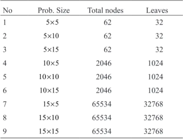
In order to compare the performance of the proposed methods, a set of test problems was generated as described in Table 1. The instances were classified based on the number of potential facilities and the number of customers.
Table 1. Characteristics of randomly generated problems.
No Prob. Size Total nodes Leaves
1 5 5× 62 32
2 5 10× 62 32
3 5 15× 62 32
4 10 5× 2046 1024
5 10 10× 2046 1024 6 10 15× 2046 1024
7 15 5× 65534 32768
8 15 10× 65534 32768 9 15 15× 65534 32768
As shown in Table 2, the number of iterations in Branch and cut based method was less than the number of iterations in Branch and bound algorithm and it was able to solve the problem faster because of using the appropriate cuts. It is well known that in regards to the time solution, the algorithm is superior that solves less MIP cases, and usually enumeration methods are slow, because they encounter too many MIP sub problems, in the above and based on our computational results we fairly reduce the MIP sub problems and it let to achieve optimal solutions in more reasonable time.
6. Conclusions
Through the paper some of the difficulties regarding to the solving mixed integer bi-level linear programming problems were described and a branch-and-cut algorithm proposed. The algorithm is based on two different cuts for mixed integer bi-level linear programming problems. The first one is the binding cut and the second is the objective cut. For the branching and fathoming rule, the extensions of an upper bound theorem of MIP problem are
Table 2. Results of 10 samples for each type problems.
No. Branch and cut based method
Branch and bound based method from (Beresnev, Branch-and-bound algorithm for a competitive facility location problem, 2013)
E.N N.I N.O Av.T E.N N.I N.O Av.T
1 33% 21% 14% 227 55% 39% 27% 513
2 45% 18% 15% 245 75% 73% 34% 678
3 37% 34% 21% 281 64% 44% 21% 691
4 15% 7% 4% 268 15% 7% 4% 839
5 38% 21% 7% 331 51% 41% 11% 880
6 43% 38% 11% 393 43% 38% 22% 818
7 22% 13% 7% 395 37% 27% 13% 1320
8 15% 11% 4% 442 43% 33% 25% 1495
applied. The first advantage of this approach is the ability to exploit the vast solvers for solving mixed integer bi-level linear programming problems. More than it, we believe that the proposed method has the ability of adopts itself with the other algorithm for improvement itself or the other algorithms that are good cases for developing the algorithm. Besides that, one can using upper bound theorems to the general bi-level programming problem to develop the algorithm would seem to be the most logical
course, or even works on primal heuristics, additional classes of valid inequalities, branching rules based on disjunctions involving more than one variable, and so on are good cases in the future works.
Competing interests
The author(s) declare(s) that there is no conflict of interest regarding the publication of this paper.
References
Achterberg, T., Koch, T., Martin, A. (2005). Branching rules revisited. Operations Research Letters, 33(1), 42-54. https://doi.org/10.1016/j. orl.2004.04.002 Colson, B., Marcotte, P., Savard, G. (2005). Bilevel programming: A survey. 4OR, 3(2), 87-107. https://doi. org/10.1007/s10288-005-0071-0
Bard, J.F., Falk, J.E. (1982). An explicit solution to the multi-level programming problem. Computer and Operations Research, 9(1), 77-100. https://doi.org/10.1016/0305-0548(82)90007-7
Bard, J.F., Moore, J.T.A. (1990). A branch and bound algorithm for the bilevel programming problem. SIAM Journal on Scientific and Statistical Computing, 11(2), 281-292. https://doi.org/10.1137/0911017
Beresnev, V.L. (2009). Upper Bounds for Objective Functions of Discrete Competitive Facility Location Problems. Journal of Applied and Industrial Mathematics, 3(4), 419-432. https://doi.org/10.1134/S1990478909040012
Beresnev, V.L. (2013). Branch-and-bound algorithm for a competitive facility location problem. Computers & Operations Research, 40(8), 2062-2070. http://dx.doi.org/10.1016/j.cor.2013.02.023
Beresnev, V.L., Melnikov, A.A. (2014). Branch-and-bound method for the competitive facility location problem with prescribed choice of suppliers, Diskretn. Anal. Issled. Oper., 21(2), 3-23.
Dempe, S. (2001). Discrete bilevel optimization problems. Technical Report D-04109, Institut fur Wirtschaftsinformatik, Universitat Leipzig, Leipzig, Germany.
Denegre, S., Ralphs, T.K. (2009). A Branch-and-Cut Algorithm for Bilevel Integer Programming. In Proceedings of the 11th INFORMS Computing Society Meeting, 65-78.
Domínguez, L.F., Pistikopoulos, E.N. (2010). Multiparametric programming based algorithms for pure integer and mixed-integer bilevel programming problems. Computers and Chemical Engineering, 34(12), 2097-2106. https://doi.org/10.1016/j. compchemeng.2010.07.032
Floudas, C.A., Pardalos, P.M., Adjiman, C., Esposito, W.R., Gümüş, Z.H., Harding, S.T., Klepeis, J.L., Meyer, C.A., Schweiger, C. A. (2013).
Handbook of test problems in local and global optimization (Vol. 33). Springer Science & Business Media.
Gümüş, Z.H., Floudas, F. (2005). Global optimization of mixed-integer bilevel programming problem. Computational Management Science, 2(3), 181-212. https://doi.org/10.1007/s10287-005-0025-1
Hansen, P., Jaumard, B., Savard, G. (1992). New branch-and-bound rules for linear bilevel programming. SIAM Journal on Scientific and Statistical Computing, 13(5), 1194-1217. https://doi.org/10.1137/0913069
Jeroslow, R.G. (1985). The polynomial hierarchy and a simple model for competitive analysis. Mathematical Programming, 32(2), 146-164. https://doi.org/10.1007/BF01586088
Mirhassani, S.A., Raeisi, S., Rahmani, A. (2015). Quantum binary particle swarm optimization-based algorithm for solving a class of bi-level competitive facility location problems. Optimization Methods and Software, 30(4), 756-768. https://doi.org/10.1080/10556788.201 4.973875
Pistikopoulos, E.N, Georgiadis, M.C, Dua, V. (2007). Multi-Parametric Programming: Theory, Algorithms, and Applications, Volume 1, Weinheim: Wiley-VCH, 1. https://doi.org/10.1002/9783527631216
Rahmani, A., Mirhassani, S. A. (2015). Lagrangean relaxation-based algorithm for bi-level problems. Optimization Methods and Software, 30(1), 1-14. https://doi.org/10.1080/10556788.2014.885519
Shi, C., Lu, J., Zhang, G., Zhou, H. (2006). An Extended Branch and Bound Algorithm for Linear Bilevel Programming. Applied Mathematics and Computation, 180(2), 529-537. https://doi.org/10.1016/j.amc.2005.12.039
Vicente, J., Savard, L., Judice, G. (1996). Discrete Linear Bilevel Programming Problem. Journal of Optimization Theory and Applications, 89(3) 597-614. https://doi.org/10.1007/BF02275351