Using Discrete System Simulation to Model and Illustrate Lean Production Concepts

(1)

Engineering Management Field Project

Using Discrete System Simulation to Model and

Illustrate Lean Production Concepts

By

Phillip B. Coleman

Spring Semester, 2012

An EMGT Field Project report submitted to the Engineering Management Program and the Faculty of the Graduate School of the University of Kansas in partial fulfillment of

the requirements for the degree of Master’s of Science

_____________________________ Tom Bowlin Committee Chairperson _____________________________ John Conard Committee Member ____________________________ Sara Hausback Committee Member Date Accepted: ____________________________

(2)

Acknowledgements

I would first like to thank the faculty and lecturers of the Engineering Management program at the University of Kansas. I have been consistently awed, not only by their ability to instruct, but also by their talent for relating the concepts presented to the current state of the world and industry. I found myself regularly applying new lessons learned to my professional labors. Secondly, I would like to thank my field project committee for their guidance and suggestions regarding the content and presentation of my research. Lastly, and mostly, I would like to thank my wife for her support and encouragement in furthering my education, for her willingness to adjust her own schedule so that I could attend classes and complete assignments, and for her discernment when I needed an editor or sounding board.

(3)

Executive Summary

Lean production systems are certainly not a new concept in the manufacturing industry. However, there are still a great number of production associates that do not yet have a true understanding of lean because the lean concepts have never been adequately demonstrated to them. Instead, lean training is often reserved for production

management, and the results are merely forced upon production operators during lean implementation events. Lack of proper training causes a lack of understanding, which prevents the associate from buying in to the implementation. Without associate buy-in, a worthy project can easily fall short of its potential.

Organizations must find a balance somewhere between sending every production associate to a full lean training course, which would be cost prohibitive, and the opposite extreme of imposing lean processes without providing any explanation whatsoever. A solution must be found that can convey the key tenets of lean quickly and effectively. Written or oral training will not always get the complete message across, or if it is fully expounding, then it is not typically concise. For this reason, the prospect of developing a set of animated simulations that would demonstrate lean concepts both quantitatively and visually was investigated.

The purpose of this research project, and for that matter this paper, is not to serve in itself as a comprehensive introduction to lean manufacturing concepts, but rather to provide a means to better illustrate some of the waste elimination principles of lean to

(4)

production associates to encourage understanding and buy-in. For the purposes of this paper, it will be assumed that the reader has already had an introduction to lean

(5)

List of Figures

Figure 1: Batch vs. One-Piece Flow ... 53

Figure 2: Batch vs. One-Piece Flow with Rework ... 54

Figure 3: Final Acceptance Testing ... 55

Figure 4: In-Process Verification ... 56

Figure 5: "Push" Production System ... 57

Figure 6: "Pull" Production System ... 58

Figure 7: Mixed Model ... 59

(7)

Introduction

In the effort to maximize operating margins, many manufacturing organizations are adopting lean production strategies to reduce their production costs. One of the focal themes behind most lean implementations is the elimination of “wastes.” These wastes are represented by the unnecessary costs associated with, among other things, overproduction, reworking or scrapping defective product, waiting on resources to become available, or surplus inventories in raw materials, work in process (WIP), or finished goods. By minimizing these wastes, the organization frees up the capital and resources that would have otherwise been allocated, and makes them available for investment in other areas that have the potential to produce greater return.

When first tasked with reviewing their existing production systems, most organizations will fail to recognize many of the wastes built in to their processes. Or an organization may acknowledge a waste, but qualify it as unavoidable or the costs as negligible. Some production processes have been in place for so long that it becomes difficult for the process owners to recognize the inefficiencies or the alternatives. Many companies’ production policies evolve continuously over a number of years by focusing on issues that are critical at any given time. Such an approach focuses on particular critical operations, and usually does not take into account the need for global analysis of problems within a manufacturing system (Shetwan, 2011).

(8)

When developing a lean system, it is recommended that each process step be viewed from the eyes of the customer. The “customer” may be represented by the end user, or simply a downstream production operation. In either case, the central question is “What value is being added from the customer’s perspective?” The only thing that adds value in any type of process – be it manufacturing, marketing, or a development process – is the physical or information transformation of that product, service, or activity into something the customer wants (Liker, 2004). In other words, “Is the customer willing to pay for it?” If the answer is “no,” then the activity is non-value added and should be targeted for elimination if possible, and if not, the costs associated with the activity should be minimized.

Current Challenges

Since lean manufacturing was first introduced to the industry, a number of techniques have been developed over the years that are each intended to eliminate or minimize wastes and non-value added production steps. Many of these techniques have been well publicized and are familiar to most professionals that have studied modern manufacturing strategies.

However, in some cases the benefits associated with a lean concept are not immediately apparent when introduced to a new audience. For instance, a production line operator, whose view is limited to the operation for which they are directly responsible, may not understand how a continuous flow or mixed model production system avoids waste. To them, batch processing similar models minimizes set up and

(9)

changeover times, and maximizes the volume of product that they are able to produce by the end of their shift. It may be difficult for them to visualize the costs savings that continuous flow can produce downstream in the production system, even if it means their workstation is slightly under-utilized. If an operator doesn’t understand a concept, they are unlikely to buy-in to the implementation of the concept. A lack of associate buy-in can prevent a worthy project from being successful.

Other lean principles are easier to conceptualize and intuition alone can explain how the principles have an advantage over more traditional production techniques. For example, it may be easy to understand how a Pull system can be more effective at avoiding overproduction costs than a Push system by tailoring the production schedule to more closely match customer demand. However, the scale of the advantage is not clear through intuition alone. This can present a challenge in justifying a lean implementation if a significant initial investment is required.

Project Objectives

The purpose of this research project will be to develop a set of tools that can be used to educate production associates (supervisors, engineers, and operators) on the benefits that can be achieved through some lean production concepts, and to help them better understand the reasoning behind the concepts. To accomplish this, a series of models will be developed to illustrate the effects of implementing lean concepts in an electronics production environment. The results will be illustrated not only by observing the quantitative effects that the lean implementation can have on key performance

(10)

indicators, but also by generating animated examples of a production system before and after implementing these lean concepts. These animations are meant to help the audience visualize the concepts at work in a continuous flow, rather than only in snapshots. For this research, the models will be developed using a discrete system simulation software package.

Lean manufacturing primarily evolved out of the Toyota Production System (TPS). Dr. Jeffrey Liker describes the principles of Toyota’s system by grouping them into four categories: Philosophy, Process, People and Partners, and Problem Solving (Liker, 2004). Some of the important benefits associated with applying lean manufacturing principles do not lend themselves to computer modeling. For example, benefits associated with employee empowerment, continuous improvement (kaizen), organizational learning,

and revised management structure, roles, and information systems are difficult to quantify or predict using simulation (Detty, 2000). However, other principles can be more easily illustrated, and their benefits quantified, through modeling. For the purpose of this research, the focus will center on what Dr. Liker described as the Process, or the waste elimination principles of lean. Specifically, the following lean concepts will be explored:

 One-piece flow

 Quality at the source (Jidoka)

 Production stops when a problem is found  Pull system to avoid overproduction

(11)

 Level production scheduling (Heijunka)  Mix model

For each of these concepts, simulation models will be generated to demonstrate, through animation, the concept at work and evaluate it against more traditional manufacturing techniques. Additionally, the quantitative effects on the following key performance indicators, defined by Detty and Yingling, will be evaluated (Detty, 2000):

 System Flow Time – Average time an assembly spends in the system from initial assembly step to departure to Finished Goods (FG). (Cycle Time)

 Order Lead Time – Time between order receipt and the arrival of corresponding finished goods at distribution for shipment.

 Time Between Completions to FG – Average time between assemblies being completed to FG. (Takt)

 Counters for Absolute Quantities – Counts of assemblies in queues, assemblies completed, assemblies rework, etc.

(12)

Literature Review

Lean and the Toyota Production System

Many of the fundamental concepts that together make up a lean production system were first explored and employed by the Toyota Motor Company. Toyota didn’t discover and implement these strategies all at once, but rather gradually recognized the opportunities for improvement, and developed these solutions as the company grew. For example, one of the key concepts of TPS, just-in-time production, was developed by the company’s founder, Kiichiro Toyoda, and another concept, jidoka or “automation

with a human touch”, was introduced by his father, Sakichi Toyoda, while developing his automated power loom (Liker, 2004).

As previously mentioned, many of these lean strategies focus on the idea of reducing and eliminating non-value added activities. The traditional approach had been to focus on the value added activities, and implement improvements in an effort to make these activities as efficient as possible. However, in most processes there are relatively few value added steps, so improving those value added steps will not amount to much gain (Liker, 2004). Toyota recognized this and observed that there were greater opportunities for improvement in focusing on the non-value added operations.

The concept of minimizing non-value added costs may appear straightforward, but many of these non-value adding steps are so entrenched into a traditional production process, that they are easily overlooked by the process owners. When developing TPS,

(13)

Toyota indentified seven wastes that they saw repeated again and again in multiple organizations. These wastes appeared in manufacturing processes, as well as in other business processes such as product development, order taking, and administration (Liker, 2004).

 Overproduction – Producing items for which there are no orders. This is a waste of both machine and labor resources, as well as a waste of raw materials and storage costs.

 Waiting – Material or labor waiting on other resources to become available in order to continue processing, which adds to overall cycle-time.

 Unnecessary Transportation or Conveyance – Moving work-in-process long distances between operations, sacrificing labor and cycle-time.

 Over Processing or Incorrect Processing – Committing more resources than necessary to process a part, either due to rework or by producing higher quality parts than needed.

 Excess Inventory – Excess raw material, WIP, or finished goods tying up resources, adding to storage costs, and risking obsolescence.

 Unnecessary Movement – Any avoidable motion an operator must make in order to complete an operation.

 Defects – Producing defective product that must be reprocessed or scrapped. The idea that these types of waste should be minimized seems intuitive enough at first glance. However, these concepts can lead to counter-intuitive truths in the real world.

(14)

For instance, it is hard for many organizations to accept that in some cases, the best solution is to idle a machine and stop producing parts. Or that it may not be a top priority to keep workers busy making parts as fast as possible. This avoids overproduction, which is the fundamental waste since it leads to so many of the other wastes. Furthermore, it may be best to build up an inventory in finished goods in order to level out the production schedule, and minimize day-to-day variation, rather than produce according to the actual fluctuating demand of customer orders (Liker, 2004). These scenarios where lean principles and intuition seem to conflict are where lean implementations tend to break down if not fully understood.

Below are some of the key tenets of lean manufacturing as described by Detty and Yingling (Detty, 2000):

 Process Stability – Establish processes that combine labor, machine, and materials to produce 100% quality products when they are needed to satisfy customer demand.

 Standardized Work – Define best practices in performing each job. It is a benchmark for improvement but never used as an individual performance-rating tool.

 Level Production – Attain capacity balance in a manner that precisely and dynamically matches customer demand. May use strategies such as multi-machine manning, and mixed model sequenced production scheduling.

(15)

 Just-In-Time – Each operation supplies parts or products to successor operations at the precise time they are demanded.

 Quality-at-the-Source – Build rather than inspect quality into the product. Achieved through systems that identify and resolve quality problems at their source.

 Visual Control – Display the operational status of the production system. Use of inventory displays.

 Production Stop Policy – Stop the production process when quality or production problems occur.

Each of these concepts was developed with the notion of minimizing the wastes that Toyota had identified.

Shortcomings of Value Stream Mapping

The Value Stream Map (VSM) is a key tool used in many lean implementation projects to identify non-value added processes and explore alternatives. The VSM is a graphic representation of a value chain that is meant to illustrate each of the process steps that must be completed in order to deliver a product or service. It captures processes, material flows, and information flows of a given product family and helps to identify waste in the system (Liker, 2004). Typically, at least two VSMs are generated. The first represents the current state of the system and is primarily used to assist the lean implementation team in understanding the entire system from beginning to end, while identifying opportunities for cost savings. The second represents the ideal future state

(16)

of the system with the non-value added steps eliminated, and waste reducing improvements implemented.

While VSM has proven to be a useful tool for visualizing the current state of a process and identifying non-value adding steps, it is not without its limitations. Creating the maps tends to be a manual, “paper and pencil” based technique used primarily to document value streams. This will limit both the level of detail and the number of different versions that can be handled (Lian, 2002). Additionally, in real-world situations, many companies are of a high variety, low volume type, which may result in composing many VSMs (Lian, 2002). Drawing these maps by hand, displaying them, and making changes to them are cumbersome processes that take a lot of time (Gurumurthy, 2011). Sometimes, the potential benefit portrayed by the maps is unrealistic. The future state map which is drawn is based on the assumption that all the issues in the problematic areas will be completely resolved (Gurumurthy, 2011). Lastly, VSM tends to better serve simple, linear, systems. Combined serial and parallel queue disciplines are difficult, if not impossible, to be treated by analytical methods (Carlson, 2008).

Because VSM is such a fundamental tool in lean planning, it is often used as a training device to illustrate the benefits of lean, or the basis behind lean concepts. However, it is static in nature, and can only capture a snapshot view of the shop floor on any particular day (Gurumurthy, 2011). This can limit the audience’s comprehension of the concepts that are being described. So as revealing as a VSM can be, many people fail to “see”

(17)

how it translates into reality. The VSM risks ending up as a nice poster, without much further use (Lian, 2002).

Merits of Simulation

One alternative to the basic VSM is the simulation model. In the simulation model, each operation contained in the VSM is represented by a module. The crucial performance details associated with the operation can be represented in the model, such as the time requirements to complete the operation, variability in time, resource requirements, maximum queue lengths, interdependencies between operations, etc. Once the model is built, the system can be simulated over a period of time to visualize how material and/or information flow during start-up, steady state, and shut-down. The system can be monitored to identify problem areas that may cause bottlenecks or starvations. Simulation through automation can provide a visual and dynamic illustration of how the system would work (Detty, 2000). Additionally, statistics on key performance indicators can be collected in order to quantify costs and savings associated with any changes that are made to the system. Simulation can offer genuine excitement by pre-testing ideas and introducing realistic “what-if” changes in the parameters (Carlson, 2008).

A simulation model can be built using a general purpose programming language (such as C++, Visual Basic, or Java), or can be built using custom software that was designed for the purpose of developing simulation models (such as Arena, Simul8, or ExtendSim). In the latter case, many times the software allows the model to be built using a graphical interface in such a way that the end product looks very much like a VSM. This allows an

(18)

audience that is unfamiliar with simulation modeling, but has had previous experience with VSM, to quickly recognize the system being modeled.

New concepts can be hard to introduce and simulation has proven to be a powerful eye-opener. Combining simulation with the visual map of VSM promotes faster adoption and less resistance to change from the workforce (Lian, 2002). As previously mentioned, VSMs can be limited in their ability to model complex systems. However, simulation is the most robust and realistic way of evaluating the performance of a system of multiple queues. Its primary use is to test changes in a system before they are implemented (Carlson, 2008). Researchers have suggested the use of simulation models in conjunction with VSM as it is an effective tool to simulate both the current state and future state of the case organization (Gurumurthy, 2011).

By collecting data on key performance indicators during the simulation of a production system, an organization can create an image of the potential quantitative effects of implementing new strategies. Without simulation, it is difficult for organizations to predict the magnitude of the benefits to be achieved by implementing lean principles. The decision to adopt lean manufacturing techniques often must be based on faith, reported experiences, and general rules of thumb. Many times, such faith-based justification is insufficient (Detty, 2000). Alternatively, simulation can help managers see the effects before a big implementation (layout change, resource reallocation, etc.) without huge investment (Lian, 2002). While the benefits associated with lean concepts cannot all be modeled, simulation can quantify the expected performance

(19)

improvements from applying continuous flow, just-in-time inventory management, quality at the source, and level production scheduling (Detty, 2000). Once the decision has been made to implement a new production approach, and the strategy has been deployed to the production floor, the results of the simulation model still provide value during the “Check” step in a Deming Plan-Do-Check-Act cycle. By comparing actual plant performance during the implementation of lean procedures to the simulation results, it provides a benchmark to judge the organization’s implementation effectiveness and the need for remedial action (Detty, 2000).

Schroer shows how simulation can be used to model the concepts of lean by simulating before and after implementations, as well as to provide the quantitative results of varying key parameters (maximum WIP, Kanban capacity, addition of resources {operators and/or machines}, process variability, etc.) (Schroer, 2004).

(20)

Project Methods

This research project began with a study of lean production strategies and the use of discrete system simulation. Through this investigation, a set of lean concepts to be simulated was selected based on how well the concepts could be illustrated using the animation and quantitative analysis tools provided by simulation. Once the concepts were identified, a set of models designed to represent each concept was developed using the steps described by Jerry Banks et al.

Model Purpose

The primary purpose of the models generated for this research was to demonstrate, rather than to simulate, lean principles in action. The production systems modeled do not represent any production systems that exist today, at least not intentionally, but rather realistic production systems that serve to highlight the concepts being presented. Nearly any real-world production system will include unique dependencies and interactions between processes that may be irrelevant to the discussion points of this research. In order to best convey the intended concepts, the modeled production systems were simplified to promote comprehension.

Data Collection

While the production systems being modeled are hypothetical and designed to better convey the desired concepts, it was preferred that they be fairly realistic so that an audience is more inclined to trust the results rather than discount the model as a

(21)

“perfect world” example that could never be realized in practice. For this reason, the models are loosely based on actual production processes at an electronics manufacturing facility. Production processes at the facility were observed and provide the template for model parameters such as the material flow, operation times, operation yields, and so on. These parameters were then adjusted as needed to emphasize the effects of the lean implementations, and to better serve as education tools. For example, defect production rates were exaggerated to better illustrate the effects of inefficient rework policies that would otherwise require long simulation runs, or multiple replications, to illustrate.

Model Formulation

For the purpose of this research, the simulation software selected to build the simulation models was ExtendSim 8. This package was preferable for the following reasons: First, the author already had experience using ExtendSim, and therefore the learning curve to develop the models was minimized. Second, ExtendSim provides a graphical interface to build the models which means the end result looks very similar to a VSM, which promotes comprehension for those unfamiliar with simulation software. And finally, Imagine That, the makers of ExtendSim provide a free downloadable demo version of the software that can run most models developed using one of the paid versions. This allowed the simulation models to be created using a paid version of the software and then run on any PC that has had the demo version installed, providing the flexibility necessary to use the models for training purposes.

(22)

Multiple models were generated, and the specific traits of each will be discussed in the Results section of this paper. However, all of the models shared the following components:

1) Clock – Each simulation run represents a single twenty-four hour day (1,440 minutes) and the primary time unit used is minutes. To increase comprehension, the simulations schedules were simplified and did not include scheduled breaks, lunch, or shift change-over.

2) Logic Structure – The logic structure varies based on the model and will be described in more detail in the Results section. However, each model was built using a graphical interface such that the process model resembles the VSM, promoting understanding for those already familiar with VSM.

3) Controlled Variables – The controlled variables also vary based on the individual model and include production parameters such as batch size, demand rate, operation time, operation yield, and so on.

4) Initial Conditions – In some models, the simulation begins with an empty, or “dry”, production line. Other models include in-process queues that are initialized with some quantity of in-process product, or a “wet” line. All equipment is assumed to be up and running at the beginning of each simulation run.

5) Termination Criteria – All models terminate at the end of the production day (i.e. after 1,440 minutes of simulation time).

(23)

6) Randomization Generator – Because these models are intended to be used to educate, the amount of random behavior had to be minimized in many cases. It would be unfortunate if a combination of randomly generated parameters caused a simulation run to produce inconclusive, or contradicting, results. Given enough replications, the results would eventually support the appropriate conclusions, but multiple replications are not practical in a training environment. Therefore, many of the parameters used in these models were defined by constants. In the cases where randomness is desired, the simulation software used, ExtendSim, includes embedded randomization generators.

7) Probabilistic Generators – As above, the use of probabilistic generators was limited due to the nature of the models, and the embedded probabilistic generators in ExtendSim were used where appropriate.

8) System Performance Data Collection – ExtendSim provides the ability to display information on key performance indicators on the model display itself so that the current information can be observed as the model is running. ExtendSim also provides the ability to log this same information to a workbook. Both of these features were utilized. The key performance indicators that are monitored are those that were discussed in the Introduction (cycle time, order lead time,

takt, and absolute counters).

9) System Performance Data Analysis – The key performance indicator information logged above was compared and contrasted before and after the lean implementation to quantify the results.

(24)

Model Validation

Because the models developed for this research are intentionally altered versions of the observed processes, there was no historical data to compare the model results to for validation. However, the graphical nature of the simulation software allows the model to be viewed as a VSM. Therefore, the model was verified and validated through careful trace studies, detailed animation to verify proper system behavior, and a review of model behavior with system experts (Detty, 2000).

Model Execution

In most of the models, random behavior was intentionally removed or minimized so that each model need only be run through a single replication to illustrate the associated concept. Additionally, the models were formulated such that a single replication of a full production day can be run at a simulation speed that, first, is slow enough to allow the audience to observe and comprehend the process in motion, and second, is fast enough that the replication completes in less than four minutes. The models will also provide the operator the ability to pause the simulation at various times as needed to point out intricacies of the process.

(25)

Results

Following is a discussion of the results of running each of the sets of completed simulation models, observing the animations, and analyzing the quantitative effect on the key performance indicators.

One-Piece Flow

The first set of simulation models was developed with the purpose of illustrating the lean concept of one-piece flow. One-piece flow challenges the popular notion that work can be performed more efficiently if multiple items are processed through a specific operation as a group or batch. Typically, the argument used to justify batch processing is that it distributes any setup or changeover costs associated with completing an operation on a certain model of product over the batch size. In other words, if items are processed in batches of ten, then the setup or changeover costs per item are ten times less than what they would be it the items were processed one at a time. Toyota recognized that setup and changeover are non-value added steps, and should therefore be eliminated, or at least minimized. If these costs can be eliminated, or made insignificant, then the benefits associated with batch processing become insignificant as well.

Production associates sometimes claim that performing an operation on a batch of items in series allows the operator to get into a “flow” or “rhythm” and therefore work faster. However, a production increase is rarely realized in practice. Additionally, an

(26)

operator’s mind may wander when they’re in a rhythm and they’re more likely to create a defect or miss an inspection step. One-piece flow can keep the operator focused on the task at hand.

Once the benefits (actual or imagined) of batch processing are removed from the decision making process, production management can focus on the benefits of one-piece flow. The most obvious benefit is that one-one-piece flow keeps product moving through the factory at all times. Products don’t sit idle in queues, waiting for additional material to arrive to satisfy a predetermined minimum lot size or a certain operation start time. Instead, the signal that work is ready to be performed is generated as soon as the first item arrives in the queue, and the item is processed as soon as the equipment and labor necessary for the next operation become available. Additionally, big buffers (inventory between processes) lead to other suboptimal behavior, like reducing motivation to continuously improve operations (Liker, 2004). The queues between processes reduce the interdependence among the workstations, which means that as long as the upstream queues are never full, and the downstream queues are never empty, there is no immediate incentive to improve the process.

The first simulation model was designed to illustrate these concepts. The model represents a production system that is comprised of four sequential workstations. The customer demand rate is such that the system will need to produce one item every 15 minutes. The total value added time required to produce a single item is 25 minutes,

(27)

but each of the workstations can perform the operation assigned to it in less than ten minutes. Initially, the workstations will be instructed to only begin work when there are a minimum of ten items in the upstream queue. Once the workstation has begun work, it will continue to work until the queue is empty at which time the station will shut down and again wait for ten more items to arrive in the queue. The minimum lot size can be adjusted during the simulation run, or between simulation runs, down to a minimum lot size of one (one-piece flow). During the simulation, information will be collected on the cycle time of the items through the production system, the number of items in the system at any given time, and the time between product deliveries to finished goods inventory (takt time). Additionally, the cycle time through the first

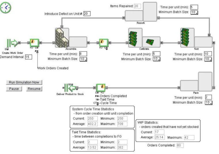
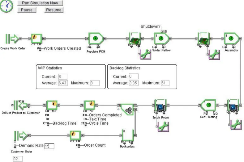
operation will also be monitored to demonstrate the time between a build order arriving on the floor, and when work actually starts. As the simulation is running, the animation will show the movement of product through the system, the size of the queues at each workstation, and real-time statistics on the performance indicators mentioned above. The graphic representation of the model is included in Figure 1.

Model Results

When the model is simulated with the minimum lot size set to ten, a few items of note become apparent right away. First, even though the first work order is delivered to the first operation immediately, work doesn’t begin until nine more orders arrive. The first operation requires eight minutes of value-added time to complete, but the first order to arrive waits 135 minutes before being processed. The tenth order to arrive must wait for the orders ahead of it in the queue to complete before being processed, so it sits in

(28)

the queue for 72 minutes. In the end, the orders require an average of just over 110 minutes to complete the first operation, representing eight minutes of value added labor. Second, by the time the first item is delivered to finished goods inventory, there are 25 items in the production system. Most of these are sitting in one of the four operation queues. There is always product sitting in at least two of the queues, and at some points in the simulation, all four queues contain product. Once the system reaches steady state, there is an average of over 19 items in the system at any time.

As mentioned above, the value added labor required to complete a single item through all four workstations is 25 minutes. However, the first item isn’t delivered to stock until 367 minutes, over six hours, after the order was delivered to the floor. The minimum cycle time for an item is 250 minutes and product requires an average of 309 minutes to arrive at finished goods after being delivered to the floor.

The final operation in the system is the pack operation, and only requires two minutes to complete. As would be anticipated, the minimum time between completions to finished goods is two minutes because once the pack operation begins working on a batch of items, it produces a delivery to finished goods every two minutes. However, once the pack operation has emptied its queue and shut down, over two hours go by before the queue has filled again and signaled the pack workstation to start up again.

A production associate that is unfamiliar with the notion of one-piece flow may be tempted to allow a few pieces to collect in a work queue before initiating action because it seems to be a more efficient use of labor, especially if there are other routine

(29)

tasks that could be done as an alternative. However, the animated model illustrates the fault in this logic. If the same reasoning is used at every step in the production system, then the wait times quickly begin to accumulate to an unacceptable level. While production management may not be concerned about an item that sits in a queue for an hour at one station, they may be more concerned once they realize that that same item sat in queues for a total of nearly six hours to complete a production system that only represented twenty-five minutes of value added time.

When the model is simulated with the minimum lot size set to one, or using one-piece flow, the results are dramatic. First, the queues become redundant because orders are pulled into the workstations for processing as soon as they arrive. Since the orders don’t spend any non-value added time waiting in queues, the cycle times through each operation, and cumulative time through the whole system, is exactly equal to the value added labor requirements. This represents a cycle time reduction of 92%. Also, since there is no WIP sitting in queues, the maximum number of orders in the production system at any time is reduced to two, nearly a 92% reduction of WIP inventory costs. Finally, the time between completions to finished goods becomes a constant that is exactly equal to the demand rate of one item every 15 minutes.

Another benefit of single piece flow is that if an undetected change in the process (equipment breakage, unacceptable material, operator error, etc.) causes an early production operation to begin to consistently produce defective material, batch processing can delay the detection of the issue, causing more defective products to be

(30)

produced before the root cause can be identified and corrected. A variation of the first model has been developed to demonstrate this concept. In this variation, an unintentional process change will cause the first workstation to begin to produce defective product after the twentieth item is complete. The workstation will continue to produce defective products until the first defect is discovered at the downstream test workstation. Once the first defect is discovered, the root cause is identified and corrected such that the first operation will begin to produce acceptable product once again. All defective products will require rework, and will then be returned to the first workstation for reprocessing. This variation of the model is shown in Figure 2.

The first replication of the model is run with the minimum lot size for each operation set to ten. Since all of the other parameters of the model are the same as the first variation, the results are exactly the same until the first defect is produced. To help the audience track the defective products through the production system, the simulation model is designed such that the defective products are represented by lightning bolt icons. This is meant to convey that these parts have been made defective by some means, possibly by electro-static discharge. The idea is that while an observer watching the simulation run can see exactly when the first defect is produced, the operators in the simulation are unaware of the defects until they’ve reached the test operation. After the first defective item is produced, it must wait in two downstream queues before arriving at the test workstation where the defect is detected, 130 minutes later. Because of this delay, 19 more defective products are produced by the first workstation

(31)

total of twenty items must be reworked and returned to the first operation. The peak cycle time for the system increases to 709 minutes, or nearly twelve hours. The peak WIP inventory level increases to 42 items, and even though the first defect occurs approximately one quarter of the way through the simulation run, the WIP levels don’t recover to their steady state level until the very end of the run. While the defective products are being repaired, 382 minutes, over six hours, elapse between consecutive deliveries to finished goods.

Again, by reducing the minimum lot size required to commence working at a workstation, the effects of one-piece flow can be observed to be significant. The first defect is detected fifteen minutes after being produced and in that short time, only one additional defect is made requiring repair. The peak cycle time is only increased by 33 minutes and the overall average cycle time increases by less than one minute. The WIP inventory level peaks at four, and recovers to steady state an hour and a half after the first defect is produced. The maximum time between completions to finished goods is 43 minutes.

The models developed here to demonstrate the advantages of one-piece flow do not specifically address the case that there may also be cost savings due to reduced setup and changeover times associated with batch processing. However, by better understanding the costs introduced by batch processing, these setup and changeover savings may be viewed in a different light. The magic of making huge gains in productivity and quality and big reductions in inventory, space, and lead time through

(32)

one-piece flow has been demonstrated over and over in companies throughout the world. This is why the one-piece flow cell is the ultimate in lean production. It has eliminated most of Toyota’s seven kinds of waste (Liker, 2004).

Quality at the Source

The next set of models was designed to demonstrate the concept of quality-at-the-source. This concept is part of a larger production principle that Toyota referred to as

Jidoka. Essentially, jidoka means building in quality as you produce the material or

“mistake proofing” (Liker, 2004). This principle traces back to Sakichi Toyoda and his inventions that revolutionized the automatic loom including a device that detected when a thread broke and would immediately stop the loom (Liker, 2004). This set of models will focus on the advantages provided by in-process verification, or in-station quality, when compared to systems that rely on final acceptance testing after all assembly operations have been completed.

Like before, these models represent a system made up of four sequential operations. The times required to complete each operation have changed slightly, and since the previous section demonstrated the advantages of one-piece flow, minimum lot sizes will not be used. In this system, every workstation is assumed to have a 10% chance of producing a defect. These defects will be generated randomly using ExtendSim’s randomization generators. As in the last model, during the animated simulation run the icon for a defective product will be changed to a lightning bolt as soon as the defect is

(33)

introduced to allow the audience to track the defects as they progress through the system. However, like before, the defect is not detected by the operators in the simulation until the appropriate test step.

Model Results

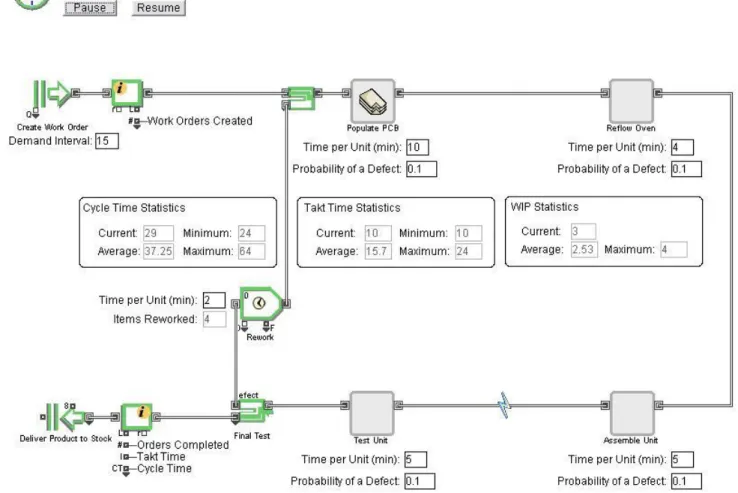
In the first model, a defect generated at any of the workstations will not be detected until the item completes the final test operation. If a defect is detected, the item is reworked and returned to the first operation for reprocessing through the system. The model can be seen in Figure 3. When watching the animation run, the audience quickly notices how much time is wasted, especially when a defect is introduced early in the production system. An item that is made to be defective at the first workstation must travel through three additional workstations before the defect is detected. At each of these workstations, additional labor is applied to the item, but this labor is wasted because the item will ultimately need to be processed through the workstation at least one more time after repairs are made. Additionally, a repaired item progressing through the production process a second time is exposed to the same probability of a defect being introduced again. As a result, an item may need to be repaired and re-processed more than once.

Since this model includes a random element, in that each operation introduces a 10% likelihood of creating a defect, the quantitative results are expected to vary slightly from run to run. Therefore, multiple replications of the simulation were run before analyzing the variable results. The production system represents 24 minutes of value added work.

(34)

Since this system was designed to use one-piece flow, as was found in the previous model, the minimum cycle time for an item requiring no rework was exactly equal to the value added time in each replication. However, the maximum cycle time was much higher, peaking at nearly 700 minutes (twelve hours) and averaging nearly 420 minutes (seven hours) across all replications. These high cycle times are due to two things. First, a large number of items must be processed through the system more than once, which will at least double the cycle time. And second, after getting repaired, units are delivered back to the first operation and may arrive while the workstation is busy processing another piece. When this happens, the new item must wait in the workstation’s queue. Additional items to arrive are also added to the queue until the workstation can process the backlog. As was observed in the previous model set, this non-value added time spent in the queue quickly impacts the average cycle time.

The first operation takes ten minutes to complete, and requires the most time of all the operations in the critical path of the system. As a result, it is also the operation that sets the fastest takt time for the system. Therefore, the minimum time between deliveries

to stock is ten minutes. If defects are introduced in consecutive items, the time between deliveries quickly increases and can peak around 60 minutes. Consecutive defects requiring reprocessing also mean that the amount of material in the system is increasing. Across multiple replications, WIP can peak as high as 18 pieces and averages around six.

(35)

Finally, an item repaired once is reprocessed and therefore exposed to the same chance of being made defective again. The ultimate first-pass yield for the system, the percentage of units that travel through the system without requiring any repair, can be as low as 30% and rarely gets above 50%.

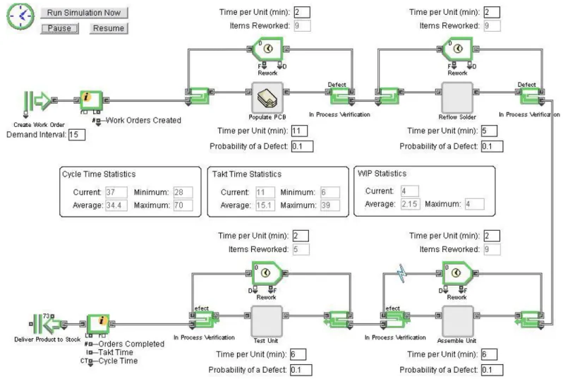
The next system model uses the exact same operations, with the same probability of generating a defect. However, this time each operation will include an inspection step with the intent of confirming that the operation that was just completed was done correctly, and no new defects were introduced. To account for the additional time required to perform the inspection step, the required labor for each operation will be incremented by one minute. If a defect is identified, then the item will be repaired, reprocessed through the current operation, and then inspected again until the item is confirmed to be acceptable. In this way, only defect free product is sent on to the subsequent workstation. This model is shown in Figure 4.

The additional four minutes of inspection time performed on all units, defective or not, mean that the minimum cycle time for all items is increased to 28 minutes. However, the average cycle time is only 34 minutes across replications and peaks at just over 100 minutes. This is a dramatic improvement when compared to the final acceptance testing example, primarily because defective products are identified immediately and no time is wasted by sending the defects on to the next workstation when they will ultimately need to be re-processed. Also, in the previous example a defect generated at any point in the system meant that the item would eventually be returned to the first

(36)

workstation, increasing the probability of a backlog. While it is still possible that backlogs can be created in this new example, they occur less often and are cleared more quickly. This means that less non-value added time is spent with items sitting in queues.

Because of the architecture of the new system, it is no longer as dependant on the labor requirements of the first operation when it comes to the minimum takt time. Instead,

the labor requirements of the final operation set the minimum takt. Also, defects

introduced in consecutive items result in less of an increase in total cycle time for the units, so the maximum time between deliveries to stock peaks at less than 50 minutes. Shorter cycle times also mean that items spend less time in the system, and as a result, there are typically fewer items in the system at any given time. The peak amount of WIP in the new system is only five items, and the average WIP level is less than two.

Finally, since an item that is found to be defective at one of the later workstations does not need to be reprocessed by an earlier workstation, it does not get re-exposed to the opportunity for a defect to be introduced. This means that the system’s average first-pass yield is increased to about 57% and rarely dips below 50%.

Pull Production System

The next lean concept explored is the “Pull” production system. Pull refers to the way in which signals to produce are delivered to the production system. In a traditional “Push” system, the anticipated customer demand is predicted and work orders are delivered to the production system at a rate that matches the estimated demand. After an order completes the first production operation, it is delivered to the next operation for further

(37)

processing. Each operation continues to produce product as long as there are orders being delivered from the upstream process. The workstations have no visibility of what is going on elsewhere in the system, and will continue to produce even if a backlog has developed downstream. Since customer demand is variable, it must be routinely reevaluated, and the production rate must be adjusted accordingly. If customer demand changes abruptly, the result can be a stock out or surplus inventory in finished goods. Many organizations will allow for large volumes in finished goods, permitting large safety stock levels, that safeguard against stock outs, and capable of handling surplus inventories.

The Pull system was inspired by American supermarkets (Liker, 2004). In most supermarkets, product is presented to the customer on the market floor. The consumption of product off the shelves acts as a signal to the clerk to restock the shelves from the storeroom. Dipping inventory levels in the storeroom act as a signal to purchase more inventory. In this way, customer demand initiates the action of the system and product is pulled through each step. In a Pull system, each workstation receives the signal to work from a downstream operation, rather than responding to an order delivered from upstream. Toyota described this as, “the preceding process must always do what the subsequent process says.” The American quality guru W. Edwards Deming said, “the next process is the customer” (Liker, 2004).

(38)

To observe the differences between Push and Pull production systems, models were creating again representing a four step production process. If customer demand were constant and predictable, then scheduling production on the factory floor would be easy, and whether a Push or Pull system were used would be inconsequential. To better illustrate the differences, the customer demand was scheduled such that it would vary over time. The customer demand rate will begin at a rate equal to the predicted demand. Then, approximately one third of the way through the simulation, the customer demand will increase by 50%, perhaps in response to a promotion or a shortage of a competitor’s product. As is often the case, a spike in demand can mean that customers’ short term needs are satisfied and therefore the spike is immediately followed by a temporary dip. Furthermore, in order to observe other effects on Push versus Pull systems, the second workstation in the system will break down for a short period of time shortly after the simulation has begun. The workstation will be shut down for two and a half hours while repairs are made.

Since the steady state performance of the system is of more interest than the startup performance, the modeled production system will be “wet,” meaning that each workstation will be initialized with a single item in its work queue, at the beginning of the simulation.

Model Results

(39)

arrives in the queue and then delivers the product to the next workstation when complete. The system will again utilize one-piece flow, and yield will not be considered since we’ve already explored the concept of quality at the source. The model can be seen in Figure 5.

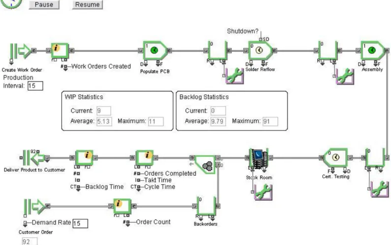
When the simulation is started, products are delivered to finished goods at the same rate as orders arrive. Finished goods inventories stay steady, and no backorders are created. Everything runs smoothly up until the point that the second workstation breaks down. Workstations downstream from the breakdown continue to produce until their supply chain has dried up, at which point finished goods inventory is consumed and backorders begin to collect. Meanwhile, the first workstation continues to produce without interruption and generates a backlog of work in the queue ahead of the workstation under repair. While the first workstation continues to produce, no product is being delivered to finished goods, so the amount of WIP steadily increases. Once the repairs are completed, the second workstation begins to work through the backlog, and the downstream operations are completed as soon as products start to flow again. The volume of backorders starts getting filled, and the backlog in front of the second workstation slowly dwindles. Ultimately, the WIP level peaks at more than double the normal operating level.

Not long after the system has recovered from the breakage, the customer demand increases by 50%. Since the push system is driven to produce at a steady rate equal to the expected customer requirements, the system doesn’t keep pace with the increased

(40)

demand. Finished goods inventory is eventually exhausted, and backorders start accumulating again. The backorders continue to accumulate until the demand falls back below the normal rate. Since the system is now producing at a rate faster than demand, the backorders are slowly filled until they’re gone, at which time finished goods inventory start to fill up to the point where there is a surplus. Inventories will continue to climb until the customer demand changes again, or the production rate is manually adjusted. This illustrates the importance of understanding customer demand well when planning a Push production system.

In the Pull system, the model is the same with the exception that the queue for each workstation will only accept a single item and then the upstream operation must wait for the queue to empty before producing more. Each operation will continuously produce while the downstream queue is empty. In this way, each workstation will only respond to signals coming from the downstream operation, rather than the upstream one. This model is shown in Figure 6.

Again, at the beginning of the simulation, everything runs well, and products are delivered to finished goods at the same rate as customer demand. Each time an item is consumed from finished goods, another item is pulled from the upstream workstation to take its place. This triggers the upstream workstation to begin working on the next item, which in turn pulls from the next workstation upstream. The pull signal propagates upstream to the first operation such that product moves through the system each time an item is consumed by a customer.

(41)

When the breakdown at the second workstation occurs, the downstream workstations continue to respond to downstream pull signals until their supply chains dry up and backorders start to accumulate as before. However, since the second workstation is no longer pulling items from the first operation, the first workstation stops producing as well. This is one of the key traits of a Pull system. If any workstation falls behind, their limited input buffer would restrict or block the upstream workstations, creating a bottleneck. If its output buffer becomes depleted, it starves the downstream operations. The blocking and starving creates interdependence among the workstations (Carlson, 2008). The stopping of production when a problem is found is also another trait of the Toyota principle of Jidoka. Since product is being pulled from the system,

but no more work is being done on new items, the WIP level actually drops to a point equal to the amount of product in the system upstream from the second workstation when the breakdown occurred. When the repairs are completed, and the second workstation begins to produce again, the downstream operations are completed as soon as items arrive since the backorders create constant signals to produce until they’re filled. Ultimately, the number of backorders and length of time they’re made to wait are about the same between the Push and Pull systems. However, the dramatic difference is in the peak WIP level. Because of the way the signals are generated in the Push system, the WIP level more than doubles while the equipment is being repaired. However, the simulation of the Pull system shows that this increase in WIP is unnecessary since it fills the backorders in the same amount of time while avoiding the additional WIP.

(42)

Shortly after the system has recovered from the workstation shutdown, the customer demand increases in the same way that it did in the first model. However, since the Pull system receives production signals that originate from the customer demand, the production rate automatically adjusts itself to exactly match that of the customer demand. Because of this, no backorders are created by the increase in customer demand, and likewise, no inventory surplus is generated when the customer demand drops.

Leveled Work Load

The final lean concept that will be explored is the notion of the leveled workload, or

Heijunka. Many times, the same logic used to justify the production of items in batches

is used to justify producing similar flavors of products in sequence. For instance, if a particular production line is capable of producing three different models of products, the production schedule may be sequenced to produce a day’s worth of the first model, then a day’s worth of the second model, and then build the third model. This may be done to reduce changeover times, or because operators prefer to work on one model type at a time, or simply because it makes the scheduling easy. Whatever the reasons, there are sometimes unanticipated disadvantages that are introduced by this type of scheduling as well. Often, different model types require different amounts of time to process through certain operations. If this is the case, then the production system will slow down when the models with the higher labor requirements are being produced, and will speed up as the less demanding models are made. This will ultimately cause

(43)

orders come in for models that are not currently in inventory, and are not scheduled to be built until later in the day, then backorders will be created. Again, many organizations will rely on safety stocks to avoid these backorders, which increase inventory costs.

Another consequence of this unleveled scheduling is that workstations that only perform operations on some, but not all, models of product will not be utilized efficiently if only one model type is built for a significant amount of time. This can be problematic if the production sequence is set based on a limited view of the system. Take, for example, the scenario where a workstation that performs an early production operation is given the authority to determine the production sequence, as long as certain production objectives are completed by the end of the shift. The operators at this workstation will produce items in an order that is most efficient to them, perhaps by grouping like models to avoid changeover. This results in a small increase in efficiency for the current workstation and a small cost savings. However, if different models require different operations to be performed further downstream in the system, then the cost savings gained through unleveled production at the early workstation may be overshadowed by additional costs downstream.

For these simulations, the models will represent a two step production process to ease comprehension. The first step is an assembly step. All orders will be processed by the same assembly workstation, but the processing time will be dependent on the product

(44)

flavor. The second step is a certification testing step that must be performed at one of three different test workstations depending on the flavor of product requiring test. Three different flavors will be produced by the system, and they be represented by green, red, and blue balls. The green products represent a low-volume, high-cost line and will require more processing time at each workstation, but will also have lower, but steady, customer demand. The blue products represent a high-volume, low-cost flavor that will require lower than average processing time at each workstation, but will have the highest customer demand. Additionally, the simulation models were constructed such that the customer demand for the blue line can be simulated either as a steady demand, or a seasonal demand. Finally, the red line will represent a mid-range line for both cost and demand. Ultimately, the build ratio will always be half blue units, thirty percent red units, and twenty percent green units.

Model Results

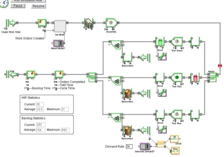
To begin to illustrate the advantages of a leveled production system, a simulation model was first developed such that the system is a Push system and the build sequence is pre-arranged. The build sequence can be easily toggled between a leveled or unleveled sequence. When the model is set to an unleveled sequence, all of the production orders for the green products for the day will be delivered to the production system first. These will be followed by all of the orders for the red products, and then finally all of the blue orders. When the system is set to a leveled schedule, orders for the different flavors will be delivered in a recurring pattern that represents the ratio of unit flavors specified above. After each unit is assembled, the items will be routed to the

(45)

appropriate certification testing workstation based on the product flavor. After the item has completed the test operation it will be delivered to the store room where it will wait for a customer order for that particular flavor to arrive. Initially, customer orders will arrive at a steady rate for each flavor such that by the end of the day an equal number of production orders and customer orders will have been processed by the system. This production system model is seen in Figure 7.

Soon after starting the simulation of an unleveled production system, a few of the disadvantages associated with this type of system become apparent. First, since the green products require more than the average amount of labor to assemble, the first workstation quickly begins to accumulate a backlog of production orders that continues to grow until the less demanding orders begin to get delivered to the system. Ultimately, the backlog peaks at eighteen orders. Second, since only the green products are being produced by the first workstation, the workstation responsible for testing the green products is quickly overwhelmed, while the red and blue test stations sit idle. And finally, even though production orders are arriving sorted by the product flavor, the customer orders are arriving at steady rate for all three flavors. The green product line is a low demand line, so not long after the production system starts up, it has produced more green items than customers have consumed, resulting in a surplus, and there are backorders for the red and blue products.

After all of the green items have been produced for the day, the system switches over to building red items. The green test station is still working to complete the backlog of

(46)

items in its work queue, and it doesn’t take long for the red test station to accumulate a backlog of its own while the blue test station continues to sit idle. New customer orders for the green items are filled from the surplus in the store room, and the volume of backorders for the red items starts to be reduced while the backorders for the blue items continue to grow. Finally the daily build for the red items is completed and the blue items begin production. By the time the blue test station finally begins to receive product to test, so much of the day has been lost that the workstation can’t complete enough orders to satisfy the customer backorders by the end of the run.

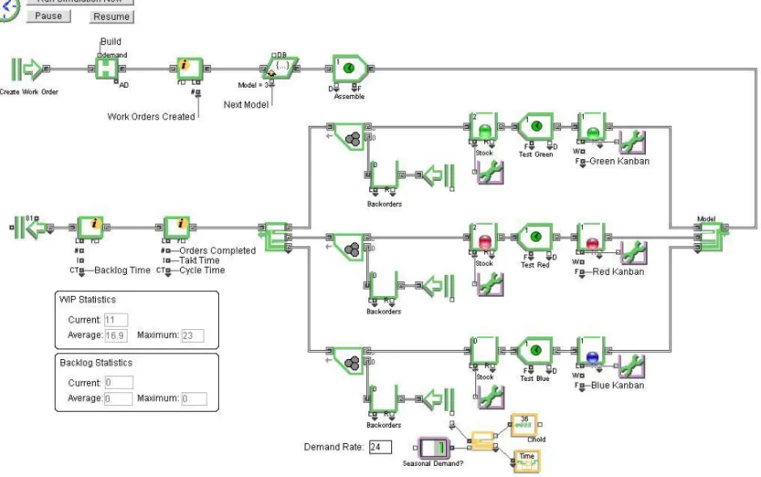
When the simulation is set to the leveled sequence, the production orders are mixed as they arrive to the system. Orders with a high labor requirement for assembly are followed by orders with low labor requirements which allows the assembly workstation to avoid long backlogs. The largest backlog is only two orders, and the station quickly recovers and reduces this backlog back to zero. Also, since the orders are mixed, product is delivered to all three test workstations regularly so that they are all well utilized while avoiding their own backlogs. In order to best utilize tools, and still keep cycle times reasonable, scheduling becomes a very important issue (Bullock, 2003). Finally, the production sequence more closely resembles the customer order rate, so there are no backorders.

Sometimes organizations have a difficult time reconciling the idea of a Pull production system with a leveled production system. This may be due to the misconception that a leveled production system requires the system to produce based on a predetermined