i
am
your
optimisation
heating, ventilation
and air conditioning
systems
The Office of Environment and Heritage (OEH) has compiled this document in good faith, exercising all due care and attention. No representation is made about the accuracy, completeness or suitability of the information in this publication for any particular purpose. OEH shall not be liable for any damage which may occur to any person or organisation taking action or not on the basis of this publication. Readers should seek appropriate advice when applying the information to their specific needs.
Published by:
Office of Environment and Heritage 59 Goulburn Street, Sydney NSW 2000 PO Box A290, Sydney South NSW 1232 Phone: (02) 9995 5000 (switchboard)
Phone: 131 555 (environment information and publications requests)
Phone: 1300 361 967 (national parks, general environmental enquiries, and publications requests) Fax: (02) 9995 5999
TTY users: phone 133 677, then ask for 131 555
Speak and listen users: phone 1300 555 727, then ask for 131 555 Email: [email protected]
Website: www.environment.nsw.gov.au Report pollution and environmental incidents
Environment Line: 131 555 (NSW only) or [email protected] See also www.environment.nsw.gov.au
Photos: OEH, AIRAH, ThinkStock & iStock ISBN 978 1 74359 990 1
OEH 2015/0317 July 2015
Foreword
This publication has been developed through an industry–government partnership between the NSW Office of Environment and Heritage’s (OEH) Energy Efficient Business (EEB) team and the Australian Institute of Refrigeration, Airconditioning and Heating (AIRAH).
It aims to support the adoption of energy-efficiency initiatives in NSW businesses and brings together expertise from both organisations and across industry.
OEH’s EEB team provides assistance to NSW businesses to reduce their energy consumption and costs, while enhancing productivity. The team has developed a suite of technology guides like this publication. These guides, which include resources on lighting, industrial refrigeration and cogeneration, are available free to download from the OEH website: www.environment.nsw.gov.au/ business.
AIRAH is an independent, specialist, not-for-profit technical organisation providing leadership in the heating, ventilation, air conditioning and refrigeration (HVAC&R) sector through collaboration, engagement and professional development. AIRAH’s mission is to lead, promote, represent and support the HVAC and related services industry and membership. AIRAH produces a variety of publications, communications and training programs aimed at championing the highest of industry standards. AIRAH encourages world’s best practice within the industry and has forged a reputation for developing the competency and skills of industry practitioners at all levels.
This publication would not have been possible without input from the following contributors – Vince Aherne (AIRAH), Mark Henderson (SEiD), Jon Clarke (Norman, Disney and Young), John Penny (Viscon Systems), Paul Bannister (Energy Action/Exergy), Lasath Lecamwasam (Engineered Solutions for Building Sustainability), PC Thomas (Team Catalyst), Andrew Smith (A.G. Coombs Advisory), Alex Koncar (Greenkon Engineering), Steve Hennessy (WT Sustainability) and Patrick Riakos (OEH).
Disclaimer
HVAC systems are complex and the extent of actual or potential energy savings will vary greatly from one HVAC system to another.
The examples and energy-savings potential discussed in this guide are not intended as
specifications for implementation, nor should they be considered to provide instruction on how to complete measurement and verification calculations for the NSW Energy Savings Scheme. It is advisable to employ specialist engineering support when developing a business case for any of the energy-efficiency opportunities outlined in this guide. OEH has a panel of specialists who will be able to assist with any optimisation project.
Foreword i
List of acronyms iv
Section 1 – Introduction 1
How to use this guide 2
Your key optimisation opportunities 3
The role of HVAC controls in reducing energy use 6
Where is energy wasted? 7
How to approach optimisation 8
Implementation 10
Potential savings 11
Simple payback period 11
Section 2 – System supervisory control optimisations 12
Opportunity 1 — Optimum start/stop programming 13 Opportunity 2 — Space temperature set points and control bands 18 Opportunity 3 — Master air handling unit supply air temperature signal 24 Opportunity 4 — Staging of chillers and compressors 29
Section 3 – Plant control parameter optimisations 34
Opportunity 5 — Duct static pressure reset 35
Opportunity 6 — Temperature reset – resetting heating hot water delivery temperature 40 Opportunity 7 — Temperature reset – resetting chilled water delivery temperature 40 Opportunity 8 — Temperature reset – resetting condenser water delivery temperature 40 Opportunity 9 — Retrofit of electronic expansion valves 45
Section 4 – Ventilation and air flow optimisations 48
Opportunity 10 — Economy cycle 49
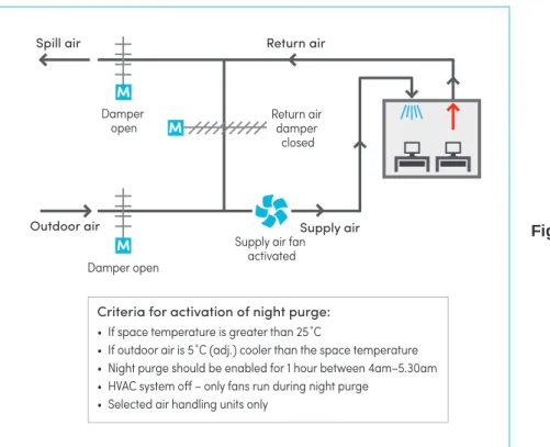
Opportunity 11 — Night purge 54
Opportunity 12 — DCV – based on controlling CO2 for occupied spaces 59 Opportunity 13 — DCV – based on controlling CO for carparks and loading docks 59
Section 5 – Variable speed based optimisations 66
Opportunity 14 — Optimised secondary chilled water pumping
(differential pressure reset) 67
Opportunity 15 — Variable head pressure control (air-cooled condensers) 71 Opportunity 16 — Variable head pressure control (water-cooled condensers) 74
Other variable speed applications for HVAC 77
Integrating multiple HVAC variable speed drive controllers 79
Section 6 – Best practice HVAC operation and maintenance 80
Opportunity 17 — Energy management planning 81
Opportunity 18 — Energy management training and awareness 86 Opportunity 19 — Energy efficiency maintenance 88 Opportunity 20 — Management of system control software 93
Section 7 – Other HVAC optimisation opportunities 95
Optimising existing fan/pump distribution systems 96
Rebalancing distribution systems 97
Duct leakage 99
Optimising boilers 99
Demand response 100
Occupancy control 100
Free cooling 100
Section 8 – Maintaining your HVAC optimisation 101
Maintaining the benefits of your optimisation 102
Appendix A: Main areas of energy waste 104
Appendix B: Documents and resources 105
Appendix C: HVAC optimisation and the NSW Energy Savings Scheme 107 Appendix D: Explaining the fan (and pump) affinity laws 109
List of acronyms
The abbreviations and acronyms used in this guide have the following meaning: AC – air conditioning
ACP − accredited certificate provider AHU – air handling unit
AIRAH – Australian Institute of Refrigeration, Airconditioning and Heating BMS – building management system
CAV – constant air volume CHW – chilled water CO – carbon monoxide CO2 – carbon dioxide CW – condenser water
DCV − demand control ventilation DDC – direct digital control
DSPR − duct static pressure reset DX – direct expansion
EC − electronically commutated EDH – electric duct heater
EEV – electronic expansion valve ESC – Energy Savings Certificate ESS – Energy Savings Scheme FCU – fan coil units
FTS − fixed time schedule GHG – greenhouse gas HHW – heating hot water HLI − high level interface
HVAC – heating, ventilation and air conditioning
HVAC&R – heating, ventilation, air conditioning and refrigeration HW – hot water
IAQ – indoor air quality
KPI – key performance indicator M&V – measurement and verification MBM − Metered Baseline Methods
NABERS − National Australian Built Environment Rating System NCC – National Construction Code
NGA – National Greenhouse Accounts NOX − nitrogen oxide
O/A – outdoor air
OEH – Office of Environment and Heritage (NSW) O&M – operations and maintenance
OSS – optimum start/stop P – proportional control
PI – proportional integral control
PID – proportional integral derivative control
PIAM&V – Project Impact Assessment with Measurement & Verification R/A – return air
RESA – Recognised Energy Savings Activities RH – relative humidity
S/A – supply air
SCHW– secondary chilled water
SMART − specific, measurable, attainable, realistic and timely TXV – thermostatic expansion valve
VAV – variable air volume VFD – variable frequency drive VSD – variable speed drive WB − wet bulb
Introduction
Heating, ventilation and air conditioning (HVAC) contributes significantly to business energy use and operating costs, typically consuming the largest proportion of energy in commercial buildings. In a commercial building, HVAC electricity consumption can typically account for around 40 per cent of total building consumption and around 70 per cent of base building electricity consumption (DCCEE Guide to Best Practice Maintenance & Operation of HVAC Systems for Energy Efficiency). Unlike other more costly energy-efficiency strategies such as plant upgrades, improving the performance of HVAC via control systems (i.e. optimisation or building tuning) can provide
immediate reductions in energy use and energy costs. The returns on investment are often able to be measured in months, not years and additional benefits can include:
• enhanced occupant comfort • improved reliability of systems • reduced ongoing maintenance costs
• improved building performance, as recognised in rating schemes such as National Australian Built Environment Rating System (NABERS) and Green Star.
Optimisation of controls is a cost-effective way to improve the efficiency and performance of HVAC systems, both in older and modern buildings. This guide has been compiled to assist those involved in facilities management, building operation and systems maintenance.
Unlike other more costly energy-efficiency strategies such as plant upgrades, improving the performance of HVAC via control systems can provide immediate reductions in your energy use and energy costs.
HVAC optimisation is sometimes as simple as changing control algorithms, altering control schedules and set points, and carrying out minor mechanical repairs and alterations to existing equipment and systems.
To achieve the benefits of optimised controls, it is essential for building owners and facility managers to see optimisation as an investment rather than a cost, while directing building
operators and service providers to include controls optimisation within their responsibilities and key performance indicators (KPIs).
Energy savings unlocked by HVAC optimisation activities can potentially generate revenue using the NSW Energy Savings Scheme. By undertaking measurement and verification, savings can be demonstrated and Energy Saving Certificates (ESCs) can be generated and sold to offset the costs of the optimisation or to facilitate future energy-efficiency interventions.
How to use this guide
The guide discusses technical concepts involved in optimising HVAC systems. It is intended to assist all those involved in the running of these systems to plan and manage energy-saving opportunities.
Energy Management Consultants Technical Service Providers
• Improve your understanding of energy-efficiency opportunities for various types of HVAC systems. • Improve value of service delivery to clients and cost-effectiveness of energy-efficiency recommendations. Building Owners
Building Managers
• Improve your understanding of potentially cost-effective energy-efficiency opportunities for your building’s HVAC system.
• Inform improvements to your HVAC maintenance scope of work to ensure ongoing energy efficiency.
Facility Managers Sustainability Managers Building Operators
• Use as a toolkit for improved operation of HVAC systems.
• Inform improvements to your HVAC maintenance scope of work to ensure ongoing energy efficiency. • Make a stronger case to building owners for investment in HVAC energy efficiency.
This guide outlines 20 HVAC optimisation strategies and how they can be applied. These strategies can save up to 50 per cent of total HVAC energy use, or up to 80 per cent of energy
Table 1 on the following page lists the 20 HVAC optimisation strategies that represent energy-saving opportunities. Guidelines are provided for optimising the control parameters within each strategy. The information provided on each strategy includes:
• a summary of the optimisation strategy
• an outline of the principle and equipment involved
• a description of current practices that may suit a particular opportunity for optimisation • an indication of the energy-saving potential and other benefits, costs and risks
• notes on the application and implementation of the optimisation.
While the guide refers to the optimisation of existing HVAC systems, the underlying control and management logic also applies to new or replacement systems. For a list of documents referenced and additional resources relevant to HVAC optimisation, refer to Appendix B.
Your key optimisation opportunities
Table 1 summarises the key optimisation strategies and provides guidance for their application for different types of HVAC systems. The energy-savings potential is specific to each strategy and non-cumulative; however, the identified energy-savings potential will naturally be greater with the adoption of two or more of these strategies.
T ab le 1 : S u mm ar y o f o pp o rt u n it ies a n d g u id e li nes a n d t he ir a pp li c a ti o n s g e O p ti m is at io n st ra te g y En e rg y -s a v in g p o tent ia l (I nd iv idu al , n o n -c um u la tiv e ) Ce nt ra l wa te r-co ol ed CH W sy ste m w /A HU s Ce nt ra l wa te r-co ol ed CH W sy ste m w/ FC Us Ce nt ra l air -co ol ed CH W sy ste m (A HU ) Ce nt ra l dir ec t ex pa nsi on (DX ) pl an ts – AH Us D uc te d dir ec t ex pa nsi on (DX ) sy ste m s Sm al l dir ec t ex pa nsi on (DX ) sy ste m s (s pl it a nd pac kage d) O pe ratio n 24 /7 Re gu la te d re lati ve hum idi ty (m us eu ms , ga lleri es et c.) Var iab le oc cu pa nc y sp ac es En close d sp ac es w ith co m bus tio n en gin es 1. O pt im um st ar t/ st op Up t o 1 0% o f t ot al e ne rg y co ns um ed b y H VA C se rvi ce s Y Y Y Y Y N N N Y N/ A 2. Sp ac e t em per at ur e set p oi nt s a nd c on tro l ban ds Up t o 2 0% o f t ot al e ne rg y co ns um ed b y H VA C se rvi ce s Y Y Y Y Y Y Y Y (Limi te d) Y Y 3. M as te r a ir h an dl in g un it ( AHU ) s up pl y ai r (S /A ) t em per at ur e sig na l Up t o 1 5% o f t ot al e ne rg y co ns um ed b y H VA C se rvi ce s Y N Y Y Y N Y Y Y Y 4. S ta gi ng o f com pr es sor s a nd chill er s Up t o 1 0% o f e ne rg y co ns um ed b y c hi lle rs Y Y Y Y N N Y Y Y Y 5. D uc t s ta tic pr es su re r es et ( D SP R) Up t o 3 0% o f e ne rg y co ns um ed b y f an s se rvi ng AH Us Y N Y N N N Y Y Y N/ A 6. T em per at ur e re set : h ot w at er ( HW ) tem per at ur e r es et Up t o 5 % o f e ne rg y co ns um ed b y H W h ea te rs Y Y Y Y 1 Y 1 N Y Y Y N/ A 7. T em pe ra tu re r es et : ch ille d w at er ( CH W ) tem per at ur e r es et Up t o 1 5% o f e ne rg y co ns um ed b y c hi lle rs Y Y Y N N N Y y (Limi te d) Y N/ A 8. T em pe ra tu re r es et : cond ens er w at er (C W ) t em per at ur e re set Up t o 1 5% o f e ne rg y co ns um ed b y c hi lle rs Y Y N Y 2 Y 2 N Y Y Y N/ A 9. R et rofi t o f el ec tron ic e xp ansi on va lve s ( EE V) Up t o 1 5% o f e ne rg y co ns um ed b y r et rofi tte d A C co mpr es so rs Y Y Y Y Y N Y Y Y N/ A 10 . E con om y c yc le Up t o 2 0% o f e ne rg y co ns um ed b y A C co mpr es so rs Y N Y Y 1 Y 1 N Y Y (Limi te d) Y N/ A
g e O p ti m is at io n st ra te g y En e rg y -s a v in g p o tent ia l (I nd iv idu al , n o n -c um u la tiv e ) Ce nt ra l wa te r-co ol ed CH W sy ste m w /A HU s Ce nt ra l wa te r-co ol ed CH W sy ste m w/ FC Us Ce nt ra l air -co ol ed CH W sy ste m (A HU ) Ce nt ra l dir ec t ex pa nsi on (DX ) pl an ts – AH Us D uc te d dir ec t ex pa nsi on (DX ) sy ste m s Sm al l dir ec t ex pa nsi on (DX ) sy ste m s (s pl it a nd pac kage d) O pe ratio n 24 /7 Re gu la te d re lati ve hum idi ty (m us eu ms , ga lleri es et c.) Var iab le oc cu pa nc y sp ac es En close d sp ac es w ith co m bus tio n en gin es 11. N ig ht p ur ge Up t o 2 0% o f e ne rg y co ns um ed b y A C com pr es sor s, du ring st ar t-up ti m e Y N Y Y Y N N N Y N /A 12 . D em an d c on tro l ve nt ila tio n ( D CV ): ca rb on d io xi de (CO 2 ) 3 Up t o 2 0% o f s pa ce c oo lin g an d h ea tin g e ne rg y re qu ire d f or p re -t re at in g o f ou td oo r a ir (O/ A) Y Y Y Y 2 Y 2 N Y Y Y N /A 13 . D CV : c ar bo n m on ox id e ( CO ) Up t o 8 0% o f e ne rg y co ns um ed b y c ar par k ve nt ila tio n f an s N /A N /A N /A N /A N /A N /A Y N /A Y N /A 14 . O pt im ise d se co nd ar y c hi lle d wa te r (S CH W ) pum pi ng Up t o 3 0% o f e ne rg y co ns um ed b y S CH W p um ps Y Y Y N N N Y Y Y N /A 15 . V ar ia bl e h ea d pre ss ure c on tro l ( ai r-co ol ed c ond ens er s) Up t o 3 0% o f e ne rg y cons um ed b y c ond ens er fa ns N N Y Y 4 Y 4 N Y Y Y N /A 16. V ar iab le h ea d pre ss ure c on tro l (w at er -c oo le d cond ens er s) Up t o 3 0% o f e ne rg y co ns um ed b y C W p um ps Y Y Y Y 2 Y 2 N Y Y Y N /A 17 . E ne rg y ma nage m en t pl ann in g Up t o 5 0% o f t ot al e ne rg y cons um ed , d ep end ing on dep th a nd c om m itmen t Y Y Y Y Y Y Y Y Y Y 18 . E ne rg y m an ag em en t t ra in in g an d a w ar en es s Up t o 1 0% o f t ot al e ne rg y co ns um ed Y Y Y Y Y Y Y Y Y Y 19 . E ner gy -e ffic ien cy m ai nt en an ce Up t o 2 0% o f t ot al e ne rg y co ns um ed b y H VA C se rvi ce s Y Y Y Y Y Y Y Y Y Y 20 . M an ag emen t of s ys te m c on tro l so ft w ar e Up t o 1 0% o f e ne rg y co ns um ed b y H VA C se rvi ce s Y Y Y Y Y Y Y Y Y Y N ot es : 1 H ot w at er s pa ce a ir h ea tin g; 2 W at er -c oo le d; 3 N ot a pp lic ab le f or 1 00 p er c en t O /A s up pl y a pp lic at io ns ( op er at in g t he at re s, p et s ho ps , m or gu es , l ab or at or ie s w ith a ni m al s, b at te ry r oo m s, e tc ); 4 A ir-co ol ed
The role of HVAC controls in reducing energy use
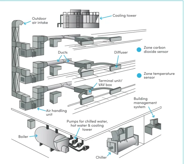
The main components of a typical HVAC commercial system are outlined in Figure 1. Central to many of the optimisation strategies outlined in this guide are the controls.
HVAC controls regulate the heating and/or air conditioning of designated areas, usually through a sensing device that compares the actual state of the space – for example, its temperature – with a target state. The control system then draws a conclusion as to what action needs to be taken – for example, start the heating element.
These control systems range from built-in proprietary controllers, to independent direct digital controls (DDC) or building-wide building management system (BMS) controls.
A BMS consists of a number of DDC that communicate via a network infrastructure and report to a computer, referred to as a head-end, supervisor or operator workstation. This central computer sends operational parameters such as set points and time schedules throughout the system and to individual plant controllers. The controllers can send back operational information such as temperature, alarms and system performance.
BMSs are also referred to as building management and control systems, building automation systems or building automation and control Systems. For consistency, the term BMS is used throughout this guide.
Figure 1: Main components of a typical commercial HVAC system Outdoor air intake Cooling tower Air handling unit Ducts Diffuser Terminal unit/ VAV box
Pumps for chilled water, hot water & cooling
tower Building management system Chiller Boiler Zone carbon dioxide sensor Zone temperature sensor
A building management system (BMS) is an
extremely valuable tool in the HVAC optimisation process
Did you know?
BMSs have steadily reduced in price over the past 30 years. They have also become more user-friendly and reliable, providing they are specified correctly, installed and commissioned by
competent personnel and their operators are trained on their functionality. Any BMS installed
within the last five to 10 years is likely to be capable of employing optimisation strategies.
The BMS is an extremely valuable tool in the HVAC optimisation process. As well as providing control logic and supervision functions, many BMSs can perform diagnostics, indicate trends and measure performance. BMSs can vary in the way they manage plant controls, the way they represent the control system and the quality and quantity of the data produced. Updating or upgrading a BMS system is often the first step in an energy-efficiency project.
It is important to ensure that optimisation capabilities of existing BMS and DDCs are taken advantage of and are not disabled. Facility operation staff need to understand the value of the optimisation and schedules need to be checked periodically to ensure they remain aligned with building use.
Refer to the Australian Institute of Refrigeration, Airconditioning and Heating’s (AIRAH) Application Manual DA – 28 Building Management and Control Systems for further information on specifying
and installing a BMS.
Modern BMSs have functions that allow KPIs to be defined and monitored, with exception reports and alarms generated for various levels of faults. In the case of HVAC system optimisation, key items should be highlighted that will initiate an alarm signal if specified operating range or limits are exceeded.
Where is energy wasted?
The structure of buildings influence energy consumption of HVAC equipment and components. The thermal performance of a building’s facade, air leakage and internal electrical loads within a building will affect the operation and performance of HVAC systems.
Energy wastage can be built into the design and construction phase of buildings. Minor alterations during operation, made to provide a quick fix for compliance or equipment problems, can
accumulate to contribute to energy waste.
This wastage is often masked by the HVAC system itself, which continues to provide adequate comfort to occupants, but at a higher energy cost.
Along with a reduction in energy use, a correctly implemented HVAC optimisation strategy can also improve tenant comfort and satisfaction
How to approach optimisation
HVAC optimisation typically involves changing control algorithms, altering control schedules and set points, and carrying out minor mechanical repairs and alterations to existing equipment and systems. The process of optimisation involves a systematic collection of information from the BMS and facilities staff, together with historic utility data and energy data collected from key items of
equipment. The analysis of energy data often uncovers inconsistencies between what is expected and what is actually happening.
An effective HVAC optimisation process relies on an engaged and informed operating and
maintenance (O&M) team, DDC or BMS control of HVAC systems and accessible, accurate HVAC documentation.
A new or upgraded BMS (achieved by programming new energy-efficiency algorithms into an existing system) can provide significant opportunities for HVAC optimisation and strategies such as optimum start/stop (OSS), economy cycles, pressure control set point reset and demand control ventilation (DCV) systems can be easy to incorporate, correct or retune.
The key to saving energy through HVAC systems is to focus on identifying and prioritising the most cost-effective opportunities and implementing them in a structured manner. It is
important to uncover and remedy the base causes of energy inefficiency in the system, rather
than just address the symptoms.
Considering that HVAC systems vary from one building to another, optimisation opportunities should be studied and analysed thoroughly, including costs of implementation, reduction of operational costs, other benefits and payback periods.
Projected benefits need to be followed up and the changes resulting from system optimisation need to be monitored. Energy-efficiency interventions should be measured and validated and this information fed back into management and maintenance decisions.
Planning should provide a logical decision-making approach to evaluate, prioritise and implement optimisations that are economically feasible. A small team of technical specialists is ideal, with direction provided by the building owner.
Identifying your opportunities
The first step towards getting the most out of your HVAC system is to identify and prioritise the key energy-savings opportunities available to your system.
Control strategies for existing systems should be reviewed by technical personnel to identify improper control sequences such as pressure and flow rate parameters, and inappropriate set points for temperature and humidity – both of which can lead to energy wastage.
There is a basic conflict between optimising the efficiency of distribution systems and optimising the efficiency of source equipment. For example, in distribution systems, raising the hot water (HW) temperature and lowering the chilled water (CHW) temperature can generate a greater temperature differential across the system, reducing required water flows and the energy used for fluid
distribution. For sources of heating and cooling, however, it is more efficient for the central plant to produce cooler HW and warmer CHW. Resolving these conflicts will result in more energy-efficient systems.
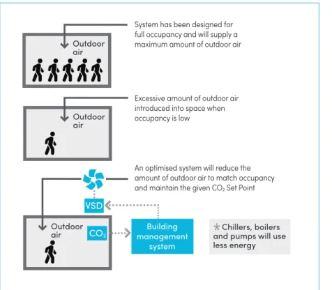
Adjusting building temperatures up or down during unoccupied periods is not a new strategy; however, it requires regular review. Using indicators of occupancy such as occupancy sensors or CO2 sensors to automatically adjust outdoor air (O/A) flows and temperature set points, or turning off equipment during periods of low occupancy, can create significant energy savings.
Did you know?
HVAC system loads primarily come from five sources:
Source Conditioning required
Building envelope Heating and cooling
Lighting Cooling
Occupancy Cooling
Equipment and appliances Cooling
Outdoor air Heating and cooling
Loads are either sensible or latent and the proportion of latent load needs to be known so that
it is appropriately managed.
Key considerations in HVAC optimisation
HVAC optimisation does not typically require much capital to implement as it focuses on the optimisation of existing systems rather than large-scale equipment upgrades and asset replacements. In addition to this, measurement and verification (M&V) of energy savings from optimisation strategies can be used to create and sell Energy Saving Certificates (ESCs) under the NSW Energy Savings Scheme (ESS), as described in Appendix C.
While estimated energy, greenhouse gas (GHG) and money savings are typically the criteria used when presenting a business case for HVAC optimisation, other factors can also influence the proposition:
• Tenant satisfaction: Will optimisation improve service quality?
• Asset value of facility: Will optimisation provide a basis for higher rent or better tenants, thereby achieving a higher asset value?
• Reliability: Will the optimised system be more reliable?
HVAC optimisation does not typically require much capital to implement as it focuses on the optimisation of existing systems rather than
large-scale equipment upgrades and asset replacements.
• Liability: Could a failure cause litigation, an insurance claim, or damage products or furnishings? • Compliance: Is the system causing non-compliance with the National Construction Code or other
mandatory requirement? Will the modification cause non-compliance or improved compliance? Funding requests for optimisation activities should be supported by robust business cases that include a cost-benefit analysis, an assessment of the return on investment and consideration of the above factors. For a comprehensive guide on building the business case, see OEH’s Energy Efficiency and Renewables Finance Guide. Each proposed optimisation measure should be carefully evaluated in terms of cost payback and indirect benefits such as improved comfort and productivity.
The HVAC optimisation process can involve significant labour costs. If the HVAC optimisation is delivered or managed using in-house staff, the implementation cost can be significantly reduced. HVAC optimisation strategies can substantially reduce energy use; however, they can also lead to unexpected results if not implemented correctly. When selecting a strategy, the complete HVAC system chain must be considered. Systems controls need to be integrated from the delivery (terminal unit) side back to the supply (central plant) side so that there is no conflict between set points and control logic.
For example, in a typical HVAC cooling system, the system chain incorporates the cooling tower, chiller, AHUs and terminal devices such as a variable air volume (VAV) box. The air flow demand of the VAV box can be influenced by the supply air (S/A) temperature, which in turn is related to the CHW temperature. This system could include a CHW temperature and an S/A temperature reset strategy. Potentially, these two control strategies, operating in conflict, could introduce instability into the cooling system.
The selection of optimisation strategies such as temperature resets should be biased towards the equipment or condition that provides the greatest energy-saving impact. The operation of multiple control strategies should be cascaded and coordinated to prevent the possibility of the benefits from one strategy being cancelled out by another.
Implementation
A range of technical service providers can assist facility managers and building owners to plan and implement individual energy-saving projects, including:
• energy management consultants
• energy efficiency maintenance providers • BMS/controls contractors
• HVAC design consultants
• HVAC contractors and maintenance providers.
The following generic steps should be followed when implementing any of the HVAC optimisation measures outlined in this guide:
Step Action
1 Prepare a technical specification for the optimisation containing performance and quality control requirements.
2 Obtain quotations from appropriate contractors (BMS, maintenance, HVAC) to do the work.
3 The selected contractor implements the optimisation(s) and demonstrates that the initiative was properly implemented and commissioned.
4 The contractor updates the system’s ‘functional description’ so that it fully reflects the new control strategies and new control parameters.
5 The maintenance contractor and facility manager are trained to understand the new control strategies and parameters, and the impacts of any variations on the operation of the HVAC system.
6 The new controls and features are added to the energy efficiency maintenance checklist so that their operation can be regularly monitored and checked as part of the routine maintenance program.
7 The system is monitored to validate the predicted energy and cost savings and the additional benefits from the optimisation.
Where multiple initiatives are being implemented simultaneously, the steps for each strategy are combined into a single implementation plan.
Potential savings
Typical scenarios of HVAC optimisation accompany a number of the opportunities outlined in this guide. These scenarios are provided for illustration only. The energy saving and simple payback period calculation examples included with these scenarios are indicative estimates of the potential savings that could result from implementation of the given optimisation scenario.
For each individual building and system, the opportunities need to be investigated in detail and a detailed business case developed. Due to the complexity and variety of possible systems and estimating the resulting savings, scenarios are not provided for all of the optimisation strategies covered in this guide.
Simple payback period
Calculating a simple payback period is the most basic of economic analysis tools and the simplest to apply. It is applicable in situations where a reduction in operating costs relative to business as usual (or some other alternative) will be achieved. Simple payback roughly calculates the number of years before capital is recovered but does not include savings beyond that time and therefore does not calculate return on investment.
Simple payback period can be calculated using the following equation: payback period (Years) = total investment ($)
savings per year ($)
If non-energy impacts and benefits are to be included in the analysis, then payback period = optimisation cost +/- non-energy impacts
annual energy savings +/- non-energy benefits
The advantages of this simple payback analysis is that it is intuitive and easily understood, does not rely on discounting and does not require a stipulated optimisation strategy life span to be defined. Other methods that will provide a more accurate estimate include net present value, internal rate of
System supervisory control
optimisations
This section provides an overview of HVAC optimisation strategies that are primarily
implemented through the supervisory control systems. This section identifies four
optimisation opportunities:
Opportunity 1
– Optimum start/stop programming
Opportunity 2
– Space temperature set points and control bands
Opportunity 3
– Master air handling unit supply air temperature signal
Opportunity 4
– Staging of chillers and compressors.
Opportunity 1 — Optimum start/stop programming
UP
TO
10
%
HVAC ENERGY
REDUCTION
Strategy summary
This strategy involves the optimisation of the HVAC system’s start and stop times. Automated starting and stopping of HVAC equipment reduces system operating hours, maintenance costs, energy costs and greenhouse gas (GHG) emissions while maintaining occupant comfort levels. An optimum start/stop (OSS) energy-saving control strategy/function uses the BMS or HVAC controller to determine:
1. the shortest period of time required to bring each zone from current temperature when systems are off, to the set point temperature.
2. how early heating and cooling can be shut off for each zone so that the indoor temperature remains within specified margins (albeit drifting).
An optimum start/stop program provides a reduction in operating hours of HVAC plant by
delaying start-up time and stopping the system sooner than the currently scheduled fixed stopping time, while still maintaining acceptable comfort conditions. Most modern building
management systems include proprietary optimum start functions. Optimum stop is typically custom-programmed.
Principle and equipment
OSS is programmed into the control system using an algorithm that needs to be linked directly to normal building time schedules and integrated with after-hours building control arrangements as well as any warm-up or cool-down programming.
Optimum start calculates the latest time to start HVAC plant and air conditioning (AC) equipment,
based on current indoor and O/A temperature conditions and historical thermal response times for the building to achieve set point, so that comfort space temperature requirements are met when occupants arrive at the scheduled occupancy time. Optimum start controls must be linked to any warm-up or cool-down control strategies.
Optimum stop calculates the earliest time to stop HVAC plant while still providing the required
comfort conditions and ventilation requirements for a building’s occupants before the scheduled end of occupancy.
The algorithm is self-adaptive as it monitors and memorises heating and cooling thermal response times of the building at various combinations of outdoor and indoor air temperatures and uses them when calculating the starting and stopping times of HVAC system.
Morning warm-up and cool-down – On days of extreme temperature, the greatest daily demand for heating or cooling may occur in the morning as the building is prepared for occupancy because a significant and rapid change in temperature is needed. The goal for an optimum start procedure is to provide as much cooling as possible to cool down the building (or heating as possible to warm up the building) for the least amount of energy possible, while avoiding demand spikes and set point overshoot.
Minimum required information
The minimum information required for an OSS program includes: • 365 day time schedule
• O/A temperature
• space or zone temperatures and set points
• OSS temperature set point (which is typically 1–2°C less than space temperature set point) • OSS enabling time (earliest time limit)
• log of recent (up to one week ago) historical data.
Minimum required equipment
The minimum equipment required for an OSS program includes: • field sensors/controllers (air temperatures, switching)
• controllers and data processors • OSS software
• trend-logging capabilities.
OSS control is generally limited to larger systems that include BMS/DDC controls, with the OSS program typically being included in the BMS software. Smaller self-contained controllers, however, can often be specified to incorporate optimum start – a cost-effective method.
Recommendation
When selecting an OSS program, several factors should be checked, the most important of
which is a full understanding of how the program calculates the starting and stopping time. It is also important to provide awareness training to HVAC system operators. The OSS function of the BMS could be disabled if HVAC operators do not know how to use it or have negative
experience with a previously unsuccessful attempt to use it.
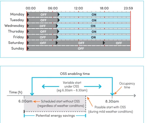
Current practice
Many existing HVAC systems are started prior to occupancy by a fixed time schedule, regardless of season, space temperature and O/A temperature (see Figure 2). For systems that do not have optimum start, HVAC plant is typically scheduled to start two to three hours before the scheduled occupancy time, all year round. For example, a HVAC system is started at 6am for scheduled occupancy starting at 8.30 or 9am, which can be extremely wasteful in energy and plant wear and tear.
During peak winter or summer conditions, early start-up of HVAC plant is required; however, starting times can be delayed during milder weather conditions. For example, if the O/A
temperature is 30°C during a hot summer morning, the plant may need to start two hours before the occupancy time. If O/A temperature in the morning is around 20°C, however, the plant’s starting time can be a lot closer to the scheduled occupancy time.
Figure 2 illustrates a very inefficient fixed time schedule that has been programmed on a BMS with HVAC starting at 6am and ending at 12pm, five days a week, every week.
Opportunity for optimisation
Introduction of a new OSS program
By using an OSS control function via the BMS, the HVAC plant automatically starts and stops on a variable time schedule. This minimises operating hours, energy consumption, energy and maintenance costs and GHG emissions. The program adjusts start/stop times by taking into account O/A temperature, space or zone temperatures and the thermal response time of the building, using adaptive learning techniques.
Optimisation of an existing OSS program
BMS programmers must ensure that:
• occupancy time is set correctly and that it matches the occupants’ needs. This should be checked and possibly re-adjusted when tenancies change
• OSS enabling time is sufficient for the seasonal air temperature requirements
• the OSS program runs together with early morning warm-up and cool-down programs to maximise the energy efficiency of the HVAC system
• the most recent (e.g. three to five days) trend-logging data is part of the calculation algorithm • space temperature limits are set correctly (e.g. no greater deviation from the temperature set
point than 2°C)
• adaptive characteristics of the OSS program minimise the time difference between occupancy starting time and the time when the OSS program achieves the required comfort space
temperature.
Figure 3 compares variable start time (6.30–8.30am) of HVAC equipment under an OSS schedule and a fixed-scheduled start time (6am) without an OSS schedule. This shows the opportunity to implement the OSS strategy and the potential energy savings. System start is selected for the latest possible time rather than a fixed time.
OSS enabling time
6.00am 8.30am
Occupancy time Scheduled start without OSS
(regardless of weather conditions)
Time (h)
Variable start under OSS (eg 6.30am – 8.30am)
Possible start with OSS (during mild weather conditions)
Potential energy savings
Monday 00:00 06:00 12:00 18:00 23:59 Wednesday Thursday Friday Saturday Sunday Tuesday OFF OFF OFF OFF
OFF OFF OFF
OFF ON ON ON ON ON OFF
Figure 2: Fixed time schedule for HVAC system on a
building management system
Figure 3: Potential energy savings of optimum start
Energy-saving potential, costs, benefits and risks
Optimising the starting and stopping of HVAC equipment requires minimal investment and is typically a very cost-effective HVAC energy-efficiency improvement. It immediately reduces the energy consumption of HVAC systems and can typically save up to 10 per cent of total energy consumed by HVAC services. Greater energy savings are expected during mild weather conditions, when plant can be started later and stopped earlier, than during extreme summer or winter weather conditions.
The full energy-saving potential will only be achieved if heating and cooling plant control is also optimised for warm-up and cool-down during OSS control.
As well as reducing the energy use of AC equipment, the OSS strategy reduces system operating hours which can also reduce maintenance costs and extend system working life.
To reduce adverse impacts on indoor air quality (IAQ) in compliance with AS 1668.2, it is important to ensure that sufficient outdoor ventilation air is supplied while the building is occupied. This can be achieved efficiently through the adoption of demand control ventilation (DCV) using carbon dioxide (CO2) sensors (refer to Optimisation Opportunity 12).
The optimum start algorithm relies on a tight building envelope which has little air infiltration and may not work well with very leaky buildings.
Application notes
The OSS HVAC optimisation strategy can be applied to any HVAC system, from the smallest room air conditioners and air-cooled split or packaged systems found in typical residential and light commercial HVAC applications, to large centralised plants with multiple chillers, air handling units (AHUs), fan coil units (FCUs) and variable air volume (VAV) boxes, found in typical commercial buildings.
Getting started
The system should be configured to achieve the outer limits of thermal comfort, typically 1 to 2°C less than the space temperature set point, rather than the exact space temperature set point. O/A intake should be minimised where possible during building warm-up/cool-down when there are no occupants and warm-up/cool-down program operation should be locked out during occupied hours. Supply air (S/A) temperature limits, of around 32–35°C (dependant on S/A diffuser type and room heights), should also be set to prevent stratification of overheated air. Building warm-up/cool-down programs can also be locked out on outdoor temperature sensing to prevent operation during mild weather.
O/A intake can be maximised in cool-down optimum start if economy mode conditions permit (see Optimisation Opportunity 11).
Minimum ventilation rates in accordance with AS 1668.2 must continue to be provided when the building is occupied. For optimum stop, chillers, boilers and valves can be turned off; however, ventilation and IAQ need to be maintained while the building remains occupied. If the heating or cooling system has a weather-compensated flow temperature program for energy efficiency, this feature should be disabled during the optimum start period, to reduce the duration of the warm-up and cool-down time.
For buildings that have gas-fired heating systems, auxiliary electric resistance heat should be locked out during the warm-up cycle.
Optimisation scenario
An office building in Sydney uses 2500 megawatt hours (MWh) of electricity and 2100 gigajoules (GJ) of natural gas per annum (pa) for its base building (house) services. The building occupancy hours are from 8.30am to 5.30pm Monday to Friday.
The BMS starts the HVAC system via a time schedule at 6am to ensure that space conditions are achieved before occupants arrive and stops it at 5.30pm.
After introduction of the OSS program and its monitoring over a year, it was found that, on average, the HVAC system would start at 7.45am and would stop at 5.15pm.
This reduction in operating hours of 120 minutes or two hours per day represented a reduction in operation of the HVAC system of 17.4 per cent. The energy savings of the HVAC system was measured as 12 per cent.
In this building, the HVAC system consumes 70 percent of the total base building electrical supply and 100 percent of the natural gas supply. The benefits of this optimisation scenario are calculated below:
Electricity saving calculation
2,500 MWh x 0.7 x 0.12 = 210 MWh pa
Assuming an average electricity cost of 15 c/kWh, or $150/MWh, the electricity cost saving is $31,500 pa
Using the National Greenhouse Accounts (NGA) factor for electricity for NSW of 1.06 tonnes (t) of CO2/MWh,
Emissions reductions = 210 x 1.06 = 223 t CO2 pa
Therefore this optimisation strategy results in an emission reduction from electricity of 223 tonnes CO2 equivalent pa.
Gas saving calculation
2100 GJ x 0.12 = 252 GJ pa
Assuming an average cost of gas of $15/GJ, the natural gas cost saving is $3,780 pa Using the NGA factor for gas for NSW of 65.4 kilograms (kg) CO2/GJ,
Emission reductions = 252 x 65.4 = 16,480 kg CO2 pa
Therefore, this optimisation strategy results in an emission reduction from gas of approximately 17 t CO2 equivalent pa.
Overall savings
Cost savings $35,280 pa
GHG emission reductions 240 t CO2 pa
Typical cost of implementation ~$5000 pa for ongoing optimisation Simple payback period 0.2 years (less than 3 months)
Additional benefits Significant water savings from reduced load on cooling towers Energy monitoring can be used as an enhancement for OSS – starting the system earlier but at a lower capacity can use less energy than starting later at high capacity, to achieve the same outcome.
Did you know?
Typically, changing the space temperature set point by 1°C can affect the energy consumption of associated cooling or heating equipment by around 10 per cent. There are actually two effects at play in such a scenario: (1) a change to the set point (or the centre point of the control
range) and (2) a change to the dead band (or the width of the control range), increasing the temperature gap between heating and cooling.
Opportunity 2 — Space temperature set points
and control bands
UP
TO
20
%
HVAC ENERGY
REDUCTION
Strategy summary
For this strategy, the space or zone temperature set points are reset and optimised to reduce the energy consumption of the associated HVAC systems, without overly compromising the comfort of building occupants.
Principle and equipment
The impact of space temperature set points and temperature control bands on the energy consumption of HVAC systems is often overlooked, even though it is one of the most simple and cost-effective ways of improving the energy efficiency of systems and buildings.
The following HVAC control parameters must be considered when optimising space temperature control for energy efficiency:
• Temperature set point – the desired temperature to be maintained.
• Dead band – the temperature band between heating and cooling, within which heating or
cooling equipment is not operated.
• Proportional band (heating or cooling) – the temperature band within which heating or cooling
equipment operates by modulating its output between 0–100 per cent. Also known as throttling range.
• Deviation – the difference between the actual (measured value) and set point. Also known as
offset.
• Differential – the difference between the switching on and switching off operating points in an
on/off type controller (a thermostat or pressure stat).
• Overshoot – the amount of excess where the actual value exceeds the target value or set point.
Energy saving is achieved by increasing the cooling-mode temperature limit to the highest acceptable space temperature and reducing the heating-mode temperature limit to the lowest acceptable space temperature, while avoiding unacceptable levels of occupant discomfort. These limits are defined by the system set points, dead band and proportional band. Widening the dead band extends the time that the system neither cools nor heats, while widening the proportional band reduces the time the system operates at full capacity.
The main limitation in setting space temperature set points and control bands is determined by occupant thermal comfort. It is the temperatures at the edges of the control band that need to be considered as well as the set point. Guidelines from Comcare, the Australian Government’s health and safety scheme for federal workers, suggest 20°C to 26°C as an acceptable temperature range
Some reference documents to assist with space temperature set points and temperature
control bands are:
• Safe Work Australia, Managing the work environment and facilities – Code of Practice
• ComCare Australia, Air-conditioning and thermal comfort in Australian public service
offices: an information booklet for health and safety representatives
• ANSI/ASHRAE Standard 55Thermal Environmental Conditions for Human Occupancy Links to these documents are found in Appendix B.
The acceptable limits for winter and summer internal temperature is dependent on numerous factors including:
• the extent of insulation on external walls • the characteristics and extent of glazing • whether window blinds are used
• the proximity of work spaces to external walls or facades • space humidity
• the type and adjustment of supply air diffusers (draughts and/or the ‘dumping’ of cold air on occupants will lead to complaints even when space temperature is acceptable)
• occupant culture: if staff can be encouraged to dress appropriately for the season, energy savings of 10-15 per cent can be typically achieved.
It is important for facility managers to discuss these issues with staff and to decide on temperature set points that are acceptable to the majority of occupants while delivering positive
energy-efficiency outcomes.
Occupants adapt to lower space temperatures in winter and higher temperatures in summer, and this effect of ‘adaptive comfort’ can be used to maximise energy efficiency by having seasonal temperature set points.
In some cases, the contractual requirements of existing leasing agreements may limit the extent of possible changes and these should be checked before any optimisations are implemented.
Recommended HVAC settings for maintaining acceptable comfort conditions with reasonable energy efficiency are:
• Winter: 20-22°C • Summer 24-26°C.
A pragmatic summer setting for an office environment is 23°C set point with 2°C dead band and 1°C proportional bands. It is also possible to have control dead bands of up to 3°C and proportional bands up to 2°C without compromising comfort conditions. The larger the dead band the larger the energy savings, but also the larger the potential for temperature variations within the occupied spaces.
It is important to note that any changes to indoor temperature ranges should be applied
gradually, for example by 0.3°C at a time, until a balance has been struck between achieving
system energy savings and maintaining an acceptable standard of thermal comfort for building
Recommendation
Preference should always be given to HVAC controllers/temperature sensors that have adjustable temperature bands and adjustable temperature step increments of 0.1°C, so
that the energy-saving potential of HVAC systems in relation to space temperature set points can be maximised.
Did you know?
Controllers use three basic behaviour types or modes: P – proportional, I – integral and D – derivative. While P and I modes are used as single control modes, a D mode is not used on its
own. The difference lies in the action of the controllers:
P – provides reliable control for stable systems
PI – helps in reducing steady state error (reduces offset)
PD – helps in achieving steady state conditions quickly (reduces overshoot)
PID – helps in reducing steady state error and also attaining steady state conditions quickly. Often, savings in energy can be gained by changing PI or PID control of temperature to P-only
control, where permissible.
PI control typically works very well in application-specific controllers supplied by manufacturers, where significant loop tuning and development has been carried out to
optimise the operation of the equipment.
A pragmatic summer setting for an office environment is 23°C set point with 2°C dead band and 1°C proportional bands.
Minimum required equipment
The level of cooling and heating provided by different air conditioning services depends on their control capabilities, control strategies and control parameters. Typically, a temperature sensor and controller regulates this duty. Temperature controllers are found in DDC-type controls and BMS, and these consist of temperature sensors and separate switching (or modulation) mechanisms with the ability to program various control algorithms that can be used for energy efficiency.
Control of space temperature is achieved by either switching heating or cooling devices on or off, or by modulating the output from HVAC equipment, based on the deviation of the space temperature from the space temperature set point, as registered by the sensor or controller.
It should be noted that different types of HVAC controllers and sensors have different capabilities and different accuracies. Some simpler thermostats cannot regulate temperature bands and have fixed differentials, fixed dead bands and adjustable temperature increment steps of 1°C only. Such thermostats are very limited in terms of implementing energy management control strategies. On the other hand, modern HVAC DDC and BMS control systems are intelligent and flexible enough to accommodate various energy-saving control strategies, including setting optimal temperature set points and control bands.
Current practice
Typical space or zone temperature set points for many commercial office buildings, shopping centres and public facilities is 22–22.5°C all year round, typically with narrow control bands. Such tight control wastes energy due of a lack of the allowable variance in temperature that is tolerated by most occupants, especially with adaptation to winter and summer conditions.
Opportunity for optimisation
Offices and similar environments
For office environments, a typical energy saving HVAC setting would be a space temperature set point of 22°C with a 2°C dead band and a 1°C proportional band for heating and a 2°C
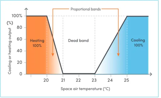
proportional band for cooling (see Figure 4). Stretch targets for energy savings are 3°C for the dead band and 2°C for the proportional band. An optimised (for energy efficiency) setting using these stretch targets would be a space temperature set point of 23°C with a 3°C dead band and a 2°C proportional band.
Figure 4 illustrates one example of an energy-efficient setting for cooling, heating and dead band temperature ranges for an office environment. Note that there is no cooling or heating between 21–23°C (dead band). Cooling modulates from 0º–100 per cent between 23–25°C, based on the deviation of space temperature from the space temperature set point (ie a 2°C cooling proportional band). When space temperature exceeds 25°C, 100 per cent cooling is engaged. Heating
modulates from 0–100 per cent between 20–21°C, based on the deviation of space temperature from the space temperature set point (i.e. a 1°C heating proportional band). When space
temperature drops below 20°C, 100 per cent heating is engaged.
Transient spaces
For transient spaces such as shopping centres, food courts, malls and foyers, space temperature set points can be more lax when compared to the comfort required for an office environment. Typical acceptable bands of control are 16–18°C (heating) and 26–27°C (cooling). This means space heating is used to maintain temperatures no higher than 16–18°C; and space cooling is used maintain space temperatures no lower than 26–27°C.
Energy-saving potential, costs, benefits and risks
Optimisation of space temperature set points and control bands is one of the most cost-effective HVAC energy-efficiency improvements. It requires minimal investment and can reduce both cooling and heating energy use (see Figure 4). For VAV systems, fan energy savings are also significant.
0 20 40 60 80 100% 20 21 22 23 24 25 Heating
100% Dead band Cooling100%
Proportional bands
Space air temperature (°C)
Cooling or
heating output
(%)
Figure 4: Typical energy
efficiency temperature set
In some cases, this strategy can immediately improve energy efficiency of the cooling/heating systems by up to 20 per cent of total energy consumed by HVAC services.
The selection of appropriate control temperatures and dead bands will also reduce the potential for heating and cooling in separate systems to operate in conflict. This can occur when spaces are served by more than one HVAC system, such as base building systems and tenants’ supplementary AC systems.
Changing the action of zone control from P+I to P-only will typically provide significant energy-efficiency gains and control stability, without compromising comfort, provided control parameters (such as set points, dead bands and proportional bands) are set properly and the system design parameters (such as air and water flow rates) are being maintained.
Comfort is king
The main risk associated with space temperature set point and control bands is an increase in temperature-related comfort complaints from building occupants. This risk can be mitigated by consulting building occupants and discussing the proposed new temperature ranges, as well as the benefits, prior to implementation. Discussions should include topics such as system controls, energy savings and seasonal clothing.
It is important that any changes to indoor temperature ranges are applied gradually to reduce the perceived impact of the change for occupants.
Application notes
Optimisation of space temperature set point and control bands can be applied to any HVAC system, from small room air conditioners and air-cooled split or packaged systems found in typical residential and light commercial HVAC applications, to large, centralised, multiple-chiller cooling plants, AHUs, FCUs and VAV boxes, found in typical commercial HVAC applications.
The wider the dead band can be adjusted to, the higher the energy savings that will be realised. This is especially applicable to open-plan-type offices served by a number of VAV boxes having re-heat capability, with the potential for conflict between adjacent boxes – one box is in cooling mode with the adjacent box in re-heating mode. Considering that the best accuracy available for space temperature sensors is likely to be ±0.3°C and their calibration tends to drift slightly after a certain time, it is recommended that a minimum dead band of 1°C is maintained with a standard target of 2°C and a stretch target of 3°C.
Similarly, a proportional band of at least 0.5–1°C is recommended with a stretch target of 2°C. The associated benefits include more stable control and higher energy efficiency; the accompanying risk is an increase of occupant complaints, which depends on the type of building and the occupancy, including the type of activities and the culture. By making small incremental adjustments and monitoring feedback, changes are likely to be more successful when occupants are given time to adapt.
Getting started
The control strategy described above is typically implemented either via the BMS or a stand-alone HVAC temperature controller, which has capabilities for altering proportional and dead bands. Once the acceptable temperature set points have been determined, a BMS or HVAC control technician should be engaged to carry out the implementation and demonstrate the success of the measure via trend-logging of the space temperature. Feedback from building occupants must also be monitored as it may be necessary to fine-tune some of the settings. Control loops must be set and tuned to provide stable and reliable control with no hunting or short-cycling of controlled equipment.
Optimisation scenario
An office building with 20,000 m² Nett Lettable Area in Sydney uses 3000 MWh of electricity and 2600 GJ of natural gas pa for its base building (house) services. The NABERS Rating is 3 stars.
Global space temperature set point for AHUs is 22°C, with the space cooling band of 22–23°C and the space heating band of 21–22°C. The air distribution system is via VAV.
By modifying the space temperature set point to 22.5°C with a 3°C dead band and 0.5°C proportional band, i.e. space cooling band to 24–24.5°C and the space heating band to 20.5–21 °C, the energy consumed by the HVAC cooling equipment (chiller electricity) is reduced by approximately 20 per cent, while the energy consumed by the boilers (natural gas) is reduced by approximately 10 per cent.
In this building, where the HVAC system accounts for 70 per cent of the total base building electricity consumption and the chillers consume 25 per cent of HVAC energy, the following benefits would be obtained:
Electricity saving calculation
Reduced electricity input for chillers: 3000 MWh x 0.7 x 0.25 x 0.20 = 105 MWh pa
Assuming an average cost of electricity cost of 15 c/kWh, or $150/MWh, the electricity cost saving is 105 x 150 = $15,750 pa
Using the NGA factor for electricity for NSW of 1.06 t CO2/MWh, Emissions reduction = 105 MWh x 1.06 t CO2/MWh = 111 t CO2 pa
As such, this optimisation strategy results in an emission reduction from electricity of 93 tonnes CO2 equivalent per annum.
Gas saving calculation
Reduced natural gas input for boilers: 2600 x 0.1 = 260 GJ pa
Assuming average cost of gas at $15/GJ, the natural gas cost saving is 260 x 15 = $3900 pa Using the NGA factor for natural gas for NSW of 65.4 kg CO2/GJ
Emission reductions = 260 x 65.4/1000 = 17 t CO2 pa
Therefore, this optimisation strategy results in an emission reduction from gas of approximately 17 t CO2 equivalent pa.
Overall savings
Cost savings $19,650 pa
GHG emission reductions 128 t CO2 pa
Typical cost of implementation ~$500 pa for ongoing optimisation
Simple payback period Less than 1 month
Opportunity 3 — Master air handling unit supply air
temperature signal
UP
TO
15
%
HVAC ENERGY
REDUCTION
Strategy summary
The aim of this optimisation strategy is to minimise the potential for simultaneous heating and cooling and reduce the amounts of cooling and heating delivered by air handling units (AHUs) and variable air volume (VAV) boxes. This strategy creates an optimised master AHU supply air (S/A) temperature signal to control the S/A temperature, minimising the mechanical cooling and heating equipment load to AHUs and VAV boxes. To achieve this, control strategies for the operation of VAV boxes and AHUs need to be well coordinated in both cooling and heating modes.
Optimised master AHU S/A temperature signals will provide a reduction in operating hours and
load of HVAC plant due to reduced needs for cooling and heating of AHUs and VAV boxes.
Principle and equipment
This strategy is applied where a central AHU delivers conditioned air to numerous VAV boxes employed to serve one or more air conditioned zones. Each VAV box serves a sub-zone, with a temperature sensor located in each zone. Multiple spaces served by one VAV box are expected to have a similar heat load and similar space temperatures, and would therefore be served by one temperature sensor located in a representative location or by multiple sensors that are averaged. Under this strategy, the BMS receives space temperature signals from each VAV zone and the VAV terminal load for each zone is determined by the deviation (or error) between the zone temperature and its associated set point. This will result in the generation of a master AHU S/A temperature signal which determines the S/A temperature. This strategy allows for differences in zone set points.
This master AHU S/A temperature signal should be based on a weighted selection of the
terminal loads. A weighted signal is used to prevent faulty VAV boxes affecting the master AHU S/A temperature signal. The weighting can be based on a simple technique such as using the
third-highest demand or a particular percentile demand. The strategy should also include the capability to ignore or blacklist known problem zones.
This master AHU S/A temperature signal determines how much cooling or heating is provided to the associated AHU and, in most cases, is controlled through the modulation of HW or CHW valves. Depending on how the master AHU S/A temperature signal is generated, the operation of re-heaters (electric duct heater [EDHs] or heating hot water [HHW] coils) can be greater or lesser. The process of optimisation must take a holistic view across VAV boxes including re-heaters, AHU fan power and chiller efficiency. The lower the AHU S/A temperature, the lower the fan energy but the higher the chiller energy consumption and the potential energy required for re-heating.