Sharif University of Technology
Scientia IranicaTransactions E: Industrial Engineering www.scientiairanica.com
A class of multi-objective mathematical programming
problems in a rough environment
A. Hamzehee
a,c;, M.A. Yaghoobi
aand M. Mashinchi
ba. Department of Mathematics, Faculty of Mathematics and Computer, Shahid Bahonar University of Kerman, Kerman, Iran. b. Department of Statistics, Faculty of Mathematics and Computer, Shahid Bahonar University of Kerman, Kerman, Iran. c. Department of Mathematics, Faculty of Basic Science, Kerman Branch, Islamic Azad University, Kerman, Iran. Received 13 August 2013; received in revised form 9 July 2014; accepted 17 January 2015
KEYWORDS Rough set; Multi-objective programming; Rough programming; Complete-optimal solutions;
Ecient solutions.
Abstract.This paper presents a set of multi-objective programming problems in a rough environment. These problems are classied into ve classes according to the location of the roughness in the objective functions or the feasible set. We study the class in which all of the objective functions are crisp and the feasible region is a rough set and, in particular, discuss the properties of the complete and ecient (Pareto optimal) solutions of rough multi-objective programming problems. In order to obtain these solutions, we need certain theorems, which we derive. Finally, we illustrate our results by examples.
© 2016 Sharif University of Technology. All rights reserved.
1. Introduction
Multiple Objective Programming (MOP) is a research eld that has been developed very much in the last three decades. It contains many real-world problems in which several objective functions have to be si-multaneously optimized [1]. Since most of the real-world problems are not crisp, the methods of classical mathematics are not usually suitable for dealing with them. Almost all concepts which we use in natural language are vague or uncertain. Some of these uncertainties are expressed by interval data, fuzziness, randomness, roughness or their hybrids.
The newest theory for the joint management of vagueness and uncertainty is that of Rough Sets Theory (RST) proposed by Pawlack [2] in 1982. It is an eective theoretical framework for discussion about knowledge that has the ability to classify objects. An object in a crisp and ordinary set is completely determined, while in a rough set, it is approximately determined based on partial knowledge. In RST, any
*. Corresponding author. Tel.: +98 3431321313
E-mail address: Hamzehee [email protected] (A. Hamzehee)
vague concept is replaced by a pair of precise concepts called the lower and the upper approximations of the vague concept. For a vague concept X, a lower approx-imation is contained in all objects which surely belong to the concept X and an upper approximation contains all objects which possibly belong to the concept X.
In recent decades, RST has been used as the fundamental tool in many applications including op-timization problems [3,4]. For the mathematical pro-gramming problems in the crisp environment, the aim is to maximize (minimize) an objective function over a certain set of feasible solutions. However, in many problems, the Decision-Maker (DM) may not be able to specify the objective and/or the feasible set, exactly. One of the ways by which DM can specify them is using RST. In [5], we proposed a type of linear pro-gramming problem with rough interval coecients, and introduced two optimal ranges (surely optimal range and possibly optimal range) and two optimal solutions concepts (completely satisfactory solution and rather satisfactory solution).
Youness [6] proposed a new type of mathematical programming problem in which the decision set was a rough set and called it rough programming problem.
He also dened two concepts for optimal solutions, namely, \surely optimal" and \possibly optimal". In his discussions, he assumed that the lower and upper approximation sets of rough sets were continuous. Osman et al. [7] classied rough programming prob-lems into three classes according to the place of the roughness. They also dened the concepts of \rough feasibility" and \rough optimality" and studied the class of rough programming problems with a crisp objective function and a rough feasible set. This paper focuses on extending this class of problems to the case when we have multi-objective functions.
There have been numerous books, monographs, articles, and chapters in books dealing with MOP problems (see [1,8] and references therein). MOP is one of the most popular methods used in Multiple-Criteria Decision-Making (MCDM). An MOP problem aims to maximize (minimize) several objective functions over a set of feasible solutions. Numerous studies of MCDM in a rough environment have been reported (for instance, see [9]). However, in this paper, we discuss MOP problems in rough environment.
In recent years, some scholars have proposed and studied dierent problems of operational research and decision-making, especially multi-objective program-ming problems, in rough environment. The newest research in this eld has been developed by Xu and his coauthors. For example, Xu and Zhao [10,11] studied a class of multi-objective decision-making problems with fuzzy rough coecients and its application in inventory problems. Xu and Yao [12,13] proposed a class of multi-objective programming problems with random rough coecients. Furthermore, Xu et al. [14] developed a Data Envelopment Analysis (DEA) model with rough parameters. Their model can be used to evaluate the performance of supply chain networks. It should be noted that in all the research, the rough coecients or parameters of problems are \rough vari-ables". The concept of rough variable, proposed by Liu [3], is dened via similarity relation in a rough space. While we discuss rough MOP problems using rough sets proposed by Pawlack [2] that are dened via indiscernibility relation as an equivalence relation in an approximation space. In other words, in the stated literature and most of the recent research, to solve rough programming problems, the scholars use the ranking methods such as the Expected value, -Optimistic value, and -Pessimistic value of rough variables to transform rough programming problems into deterministic programming ones. But we will state a methodology which transforms rough program-ming problems into classical programprogram-ming problems by changing the feasible set into its lower or upper approximations.
Recently, Tao and Xu [15] proposed a new type of rough MOP problems. They investigated the
proper-ties of feasible and ecient solutions and used \rough membership functions" to obtain a solution. They also obtained compromise solutions by using the interactive fuzzy satisfying method.
Li et al. [16] proposed a rough programming model based on the synthesis eect by distinguishing direct eect and indirect eect. They considered the role of equivalence classes in decision-making, which provides a useful tool for processing the roughness with dierent ideas. Li et al. [17] discussed the necessity and feasibility of developing a rough programming model. Their model is developed on the basis of the greatest compatible classes and synthesis eect.
In comparison with the successful application of rough set theory in real world, the research on rough programming is at the starting point. Furthermore, most of the recent achievements in rough programming have been stated based on rough variables, rough membership functions, or the eect of equivalence classes. In this paper, we further consider and analyze solutions to rough MOP problems based on upper and lower approximations of rough sets without use of rough membership functions.
The rest of the paper is organized as follows. In Section 2, some basic preliminaries about RST, MOP problems, and weighted sum method are presented. In Section 3, rstly, Single-Objective Programming (SOP) problems in rough environment are reviewed. Then, rough multi-objective programming problems are clas-sied into ve classes; and new solution concepts are dened and discussed. Finally, concluding remarks are given in Section 4.
2. Preliminaries
In this section, we recall some basic concepts, deni-tions, and theorems of RST and MOP (for more details, see [1,2]).
2.1. Rough sets
The main idea of RST is based on the indiscernibility relation that every object is associated with a certain amount of information and the object can only be expressed by means of some obtained information. Therefore, objects with the same or similar information can be indiscernible with respect to the available information. A fundamental concept in RST is the approximation space. It involves the construction of a system of denable sets.
Suppose U be a nite nonempty set of objects, and E U U be an equivalence relation on U. Then, the ordered pair A = (U; E) is called an approximation space generated by E on U. The equivalence relation E forms a partition on U like U=E = fE1; E2; :::; Erg
where for all i = 1; 2; :::; r, Ei U, Ei 6= ;,
is called an equivalence class of the approximation space A. In RST, every subset M U is described by the equivalence classes of A. Generally, two sets characterize the set M called the lower and the upper approximations of M, which are dened by the relation E, respectively, as follows:
E(M) =
[
fEi U=E j Ei Mg;
E(M) =[fE
i U=E j Ei\ M 6= ;g:
Clearly, the lower approximation E(M) is the greatest
denable set contained in M, and the upper approxi-mation E(M) is the least denable set containing M.
Also, the dierence between the upper and the lower approximations is called the boundary of M and is denoted by MBN = E(M) E(M). If MBN 6= ;,
then the set M is rough (inexact), otherwise the set M is crisp (exact).
2.2. Multi-objective programming
Any problem which optimizes multiple mathematical objective functions simultaneously under a given set of solutions is called a Multiple Objective Programming (MOP) problem and can be formulated as follows:
max f(x) = (f1(x); f2(x); : : : ; fp(x))
s:t: x 2 X; (1)
where x = (x1; x2; : : : ; xn)tis an n-dimensional vector
of decision variables, fi(x) for i = 1; :::; p is given
real-valued objective functions, and X is a feasible set of solutions.
If we directly apply the notion of optimality for SOP problem to MOP Problem (1), we obtain the following notion of a completely optimal solution. Denition 2.1 [1]. x 2 X is called a completely
optimal solution of Problem (1) if fi(x) fi(x) 8 i =
1; :::; p; 8 x 2 X.
However, when the objective functions conict with each other, a completely optimal solution does not always exist. Hence, new solution concepts, called ecient and weak ecient solutions, are introduced in MOP problems.
Denition 2.2 [1]. x2 X is called ecient (Pareto
optimal) solution of Problem (1) if there is no other x 2 X such that fi(x) fi(x) for i = 1; : : : ; p, and
fk(x) > fk(x) for at least one k 2 f1; :::; pg.
Denition 2.3 [1]. x 2 X is called weak ecient
solution of Problem (1) (weak Pareto optimal) if there is no x 2 X such that fi(x) > fi(x) for i = 1; :::; p.
2.3. The weighted sum method
One of the traditional approaches for solving an MOP problem to nd ecient and weak ecient solutions is scalarization. A simple possible way for scalarization is the weighted sum method. This method solves the following SOP problem:
max
p
X
j=1
wjfj(x)
s:t: x 2 X; (2)
where w = (w1; :::; wp) 0 is a vector of weighting
coecients assigned to the objective functions by the DM.
The relationships between an optimal solution of Problem (2) with ecient and weak ecient solutions of Problem (1) are given by the following theorems. Theorem 2.1 [1]. Let x2 X be an optimal solution
of Problem (2). The following statements hold.
If w > 0, then x is an ecient solution of Problem
(1);
If w 0, then x is a weak ecient solution of
Problem (1);
If w 0 and x is a unique optimal solution
of Problem (2), then x is an ecient solution of
Problem (1).
Theorem 2.2 [8]. In Problem (1), assume that f1; :::; fp are concave functions and X is a convex set.
If x 2 X is a weak ecient solution of Problem (1),
then x is an optimal solution of Problem (2) for some
w 0.
3. Single and multi-objective programming problems in rough environment
In this section, initially, we review some denitions and theorems of rough SOP problems. Then, rough multi-objective programming problems are discussed. 3.1. Rough single-objective programming A new type of programming problems in rough environ-ment was introduced by Osman et al. [7]. They classi-ed rough programming into three classes according to the place of roughness. In the rst class, the objective function is crisp while the feasible set is a rough set [7]. Suppose that A = (U; E) is an approximation space generated by an equivalence relation E on the set U and U=E = fE1; E2; :::; Erg is the partition
generated by E on U. Then, a rough SOP problem of the rst class is as follows:
max f(x) s:t: x 2 M
E(M) M E(M); (3)
where M U is a \rough set" in the approximation space A = (U; E) as the feasible region of the problem. The sets M= E(M) and M
= E(M) are the upper
and the lower approximations of M with respect to equivalence relation E, respectively. The function f : M! R is a crisp real valued objective function which
is continuous on M. Also, let MBN = M M be
boundary of M.
In Problem (3), the optimal value is a rough number and the optimal solutions set is a roughly-dened set (for more details about denition of rough number and rough function, see [18]).
Denition 3.1 [7]. In Problem (3), the optimal value of the objective function is a rough number denoted by f, whose lower and upper bounds are denoted by f and f, respectively.
To solve rough programming problems, the con-cepts like rough feasibility and rough optimality were dened. We quote some denitions and a theorem from [7] for Problem (3).
The solutions of Problem (3) are divided to dierent rough feasibility groups as follows [7]:
A solution x is surely-feasible if it belongs to the lower approximation of the feasible set, i.e. x 2 M;
A solution x is possibly-feasible if it belongs to the upper approximation of the feasible set, i.e. x 2 M;
A solution x is surely-infeasible if it does not belong to the upper approximation of the feasible set, i.e. x =2 M.
Other categories of the solutions are based on rough optimality, as follows [7]:
A solution x is surely-optimal if f(x) = f;
A solution x is possibly-optimal if f(x) f;
A solution x is surely-not optimal if f(x) < f.
In order to compute the lower and upper bounds for the optimal value of objective function f, we recall the following theorem from [7].
Theorem 3.1 [7]. In Problem (3), the lower and upper bounds of the optimal objective value f are given by:
f= supfa; bg and f= supfa; cg;
where (assuming the existence of the solution to the following crisp problems):
a = max
x2M f(x);
c = max
x2MBN f(x);
b = sup
Ei2U=E
EiMBN
min
x2Eif(x) :
Denition 3.2 [7]. In Problem (3), there are four optimal sets covering all possible degrees of feasibility and optimality, as follows:
F Oss = fx 2 M j f(x) = fg is the set of all
surely-feasible and surely-optimal solutions;
F Osp = fx 2 M j f(x) fg is the set of all
surely-feasible and possibly-optimal solutions;
F Ops = fx 2 M j f(x) = fg is the set of all
possibly-feasible and surely-optimal solutions;
F Opp = fx 2 M j f(x) fg is the set of all
possibly-feasible and possibly-optimal solutions. 3.2. Rough multi-objective programming
In this section, the MOP problems in rough environ-ment are investigated. We call them Rough Multiple Objective Programming (RMOP) problems, where the roughness may appear in dierent ways. In other words, the feasible set and/or the objective functions may be rough or crisp. Thus, RMOP problems can be classied as follows:
(a) MOP problems with rough feasible set and crisp objective functions;
(b) MOP problems with crisp feasible set and rough objective functions;
(c) MOP problems with rough feasible set and rough objective functions;
(d) MOP problems with crisp feasible set and both crisp and rough objective functions;
(e) MOP problems with rough feasible set and both crisp and rough objective functions.
To solve RMOP problems, we use the concepts of rough feasibility and rough optimality based on the results of Osman et al. [7] for rough SOP problems. However, we only consider an ROMP problem of the rst class (a), where the objective functions are crisp and feasible set is rough.
Similar to rough SOP problems, let A = (U; E) and U=E = fE1; E2; :::; Erg be the approximation
space and the partition generated by equivalence re-lation E on the set U, respectively. Then, the problem can be formulated as follows:
max f(x) = (f1(x); f2(x); : : : ; fp(x))
s:t: x 2 M
E(M) M E(M); (4)
where M U is a Rough set as the feasible region of Problem (4). The sets M = E(M), M = E(M),
and MBNhave the same denitions as those in Problem
(3) of Section 3.1. For all j = 1; 2; :::; p, the functions fj : M! R are crisp real valued objective functions,
which are continuous on M.
Firstly, the following example (taken from [6] with small modications) is presented as a real problem to show an instance in Problem (4).
Example 3.1. Assume the drugs D1 and D2 were developed to treat liver cancer. Let f and g be the eects of the drugs D1 and D2, respectively. In other words, if U is the set of all cells of the liver then f and g are two functions of U on the real numbers set R. Moreover, the values f(x) and g(x) mean the eects of D1 and D2 on the cell x of U, respectively. Suppose:
1. Using drugs for a year implies to kill 30% of cancer cells;
2. Using drugs for 2 years implies to kill 50% of cancer cells and 1% of normal cells;
3. Using drugs for 3 years implies to kill 70% of cancer cells and 2% of normal cells;
4. Using drugs for 4 years implies to kill 99% of cancer cells and 3% of normal cells.
Equivalence relation E on U is dened as follows:
(u; v) 2 E , 8 > > > < > > > :
u and v are killed in the same year or
u and v are not killed in the end of treatment.
Now, let M U be the set of all cancer cells. The dened equivalence relation E makes a partition to U as:
E1= fu 2 Mju was killed in the rst yearg;
E2= fu 2 M; v 2 U r Mju and v were killed in
the second yearg;
E3= fu 2 M; v 2 U r Mju and v were killed in
the third yearg;
E4= fu 2 M; v 2 U r Mju and v were killed in
the fourth yearg;
E5= fv 2 U r Mjv were not killed in
the end of treatmentg:
Then, set M is a rough set with respect to equivalence
relation E, such that the lower and upper approxima-tions of M are E(M) = E1 and E(M) = E1[ E2[
E3[ E4, respectively.
The problem of nding the maximum eect of each drug D1 and D2, is a rough bi-objective program-ming and is formulated as follows:
max ft(x)
max gt(x)
s:t: x 2 M
E(M) M E(M);
where ft; gt : M ! R are the eects of the drugs on
cell x 2 M in a certain year t 2 f1; 2; 3; 4g.
With regard to the rough SOP, we present the next denition.
Denition 3.3. In Problem (4), the optimal value of the objective function is a rough number denoted by f = ( f1; f2; :::; fp), whose lower and upper bounds
are denoted by f = ( f1; f2; : : : ; fp) and f =
( f1; f2; : : : ; fp), respectively.
Remark 3.1. If f = f, i.e. fj = fj, for all j =
1; 2; : : : ; p, the optimal value is exact, otherwise it is rough.
In order to deal with Problem (4), we need to nd the optimal values and solutions for each rough SOP Problem (5), for all j = 1; 2; :::; p:
max fj(x)
s:t: x 2 M (5)
E(M) M E(M):
With regard to Section 3.1, the lower and upper bounds of each optimal objective value fj for Problem (5) are
given by:
fj = supfaj; bjg and fj= supfaj; cjg;
where (assuming the existence of the solution to the following crisp problems):
aj= maxx2M
fj(x);
cj = maxx2M
BNfj(x) and
bj = sup Ei2U=E
EiMBN
min
x2Eifj(x)
:
and surely-optimal", \surely-feasible and possibly-optimal", \possibly-feasible and surely-possibly-optimal", and \possibly-feasible and possibly-optimal" solutions of Problem (5) by F Oj
ss; F Ojsp; F Ojps, and F Ojpp,
respec-tively.
In what follows, we extend the notions of feasi-bility and optimality of rough SOP problems to the multiple case.
Denition 3.4. For Problem (4):
^x is a surely-complete optimal solution if fj(^x) =
fj, for all j = 1; :::; p;
^x is a possibly-complete optimal solution if fj(^x)
fj, for all j = 1; :::; p.
Similar to Denition 3.2, we can dene four optimal sets covering all possible degrees of feasibility and complete optimality as follows:
F Os(sc)= fx 2 Mj fj(x) = fj; j = 1; :::; pg is the
set of all surely-feasible and surely-complete optimal solutions;
F Os(pc) = fx 2 M j fj(x) fj; j = 1; :::; pg is
the set of all surely-feasible and possibly-complete optimal solutions;
F Op(sc) = fx 2 M j fj(x) = fj; j = 1; :::; pg is
the set of all possibly-feasible and surely-complete optimal solutions;
F Op(pc) = fx 2 M j fj(x) fj; j = 1; :::; pg is
the set of all possibly-feasible and possibly-complete optimal solutions.
Proposition 3.1. For Problem (4), the following statements hold:
(i) F Os(sc)=Tpj=1F Ojss;
(ii) F Os(pc)=Tpj=1F Ojsp;
(iii) F Op(sc)=Tpj=1F Ojps;
(iv) F Op(pc)=Tpj=1F Ojpp:
Proof. The proof is straight forward.
Often, the sets F Os(sc); F Os(pc) and F Op(sc) are
empty. In other words, surely- and possibly-complete optimal solutions do not always exist. Therefore, we introduce another concepts instead of complete optimal solutions for RMOP problems. These solution concepts are based on eciency (Pareto optimality). To nd surely- and possibly-ecient solutions, we use the union of the sets F Ojss; F Ojsp; F Ojps, and F Ojpp. Hence, for Problem (4), the following notations are used:
P =
p
[
j=1
F Oj
ss; Q = p
[
j=1
F Oj sp;
S =
p
[
j=1
F Oj
ps; and T = p
[
j=1
F Oj pp:
Denition 3.5. For Problem (4):
^x 2 M is called a surely-ecient solution if:
^x 2 M and there is no other x 2 M such that
fi(x) fi(^x) for i = 1; : : : ; p, and fk(x) > fk(^x) for
at least one k 2 f1; : : : ; pg;
^x 2 M is called a possibly-ecient solution if: ^x 2 M and there is no other x 2 M such that
fi(x) fi(^x) for i = 1; : : : ; p, and fk(x) > fk(^x) for
at least one k 2 f1; : : : ; pg.
We show that if the sets P; Q; S; and T are nonempty, then the surely and possibly-ecient solu-tions belong to these sets. Therefore, the sets M and
M in Denition 3.5 can be restricted to P (or Q) and
S(or T ), respectively.
Proposition 3.2. For Problem (4), the following statements hold:
- If P 6= ;, then each member of Mr P cannot be a
surely-ecient solution;
- If Q 6= ;, then each member of Mr Q cannot be a
possibly-ecient solution;
- If S 6= ;, then each member of Mr S cannot be a
surely-ecient solution;
- If T 6= ;, then each member of Mr T cannot be a
possibly-ecient solution.
Proof. We prove only the rst item. The other items can be proved similarly. It should be proved that for every x 2 MrP , there exists ^x 2 P such that fi(^x)
fi(x) for i = 1; :::; p, and fk(^x) > fk(x) for at least one
k 2 f1; :::; pg, or equivalently:
(fi(^x) fi(x) for i = 1; : : : ; p) and
(f1(^x); :::; fp(^x)) 6= (f1(x); :::; fp(x)) :
To this end, on the contrary suppose that there is x 2 Mr P such that for all x 2 P :
(9j 2 f1; :::; pg : fj(x) < fj(x)) or
(f1(x); :::; fp(x)) = (f1(x); :::; fp(x)) :
Firstly, if fj(x) < fj(x) for x 2 P; then fj(x) = fj=
supfaj; cjg < fj(x). The following two cases can be
considered:
(i) If aj cj, then fj = aj = max
x2Mfj(x) < fj(x),
(ii) If aj < cj, then maxx2M
fj(x) = aj < cj = fj
<
fj(x), which is a contradiction since x 2 M.
Secondly, if (f1(x); : : : ; fp(x)) = (f1(x); :::; fp(x))
then fj(x) = fj for j = 1; :::; p, since x 2 P and
fj(x) = fj for j = 1; :::; p. Thus, x 2 F Ojss for j =
1; :::; p. So, x 2Tpj=1F Oj
ss Spj=1F Ojss = P , which
is a contradiction since x 2 Mr P . This completes
the proof.
According to Proposition 3.2, if the sets P; Q; S; and T are nonempty, then the rough ecient solutions of RMOP problems are restricted to these sets. Hence, we can modify Denition 3.5 as Denition 3.6 to cover all possible degrees of feasibility. It should be noted that usually among the sets P; Q; S and T , only the set P is empty.
Denition 3.6. For Problem (4):
x is called a surely-feasible and surely-ecient solu-tion if:
x 2 P and there is no other x 2 P such that fi(x) fi(x) for i = 1; :::; p, and fk(x) > fk(x)
for at least one k 2 f1; :::; pg;
x is called a surely-feasible and possibly-ecient solution if:
x 2 Q and there is no other x 2 Q such that fi(x) fi(x) for i = 1; :::; p, and fk(x) > fk(x)
for at least one k 2 f1; :::; pg;
x is called a possibly-feasible and surely-ecient solution if:
x 2 S and there is no other x 2 S such that fi(x) fi(x) for i = 1; :::; p, and fk(x) > fk(x)
for at least one k 2 f1; :::; pg;
x is called a possibly-feasible and possibly-ecient solution if:
x 2 T and there is no other x 2 T such that fi(x)
fi(x) for i = 1; :::; p, and fk(x) > fk(x) for at least
one k 2 f1; :::; pg.
Remark 3.2. If the relations of all items in the Denition 3.6 are replaced by >, then the expression \ecient" should be replaced with \weak ecient". For instance:
x is called a surely-feasible and possibly-weak e-cient solution of (4) if:
x 2 Q and there is no other x 2 Q such that fi(x) > fi(x) for i = 1; :::; p.
Notation. We denote the ecient sets in terms of four optimal sets covering all possible degrees of feasibility and optimality of the solutions as:
F Os(se): The set of all feasible and
surely-ecient solutions;
F Os(pe): The set of all surely-feasible and
possibly-ecient solutions;
F Op(se): The set of all possibly-feasible and
surely-ecient solutions;
F Op(pe): The set of all possibly-feasible and
possibly-ecient solutions.
Proposition 3.3. For Problem (4), the following statements hold:
(i) F Os(sc) F Os(se);
(ii) F Os(pc) F Os(pe);
(iii) F Op(sc) F Op(se);
(iv) F Op(pc) F Op(pe):
Proof. The proof is straight forward.
As mentioned before, the traditional approach to solve an MOP problem is scalarization and one of the most popular scalarization methods is the weighted sum method. The following theorems are stated for nding surely and possibly-ecient solutions of the RMOP problems.
Theorem 3.2. Let x be an optimal solution of the
crisp Problem (6). If wj > 0 for j = 1; : : : ; p, then
x is a surely-feasible and surely-ecient solution of
Problem (4). max
p
X
j=1
wjfj(x)
s:t: x 2 M
fr(x) = fr; (6)
where r 2 f1; : : : ; pg.
Proof. Since xis an optimal solution of Problem (6),
then it is feasible. Thus, x 2 M
and fr(x) = fr.
So, x 2 P = Sp
j=1F Ojss. Now, on the contrary
suppose that there is x 2 P such that fi(x) fi(x)
for i = 1; :::; p, and fk(x) > fk(x) for at least one
k 2 f1; :::; pg. If r = k, then fr(x) > fr(x) = fr.
Therefore, fr(x) > fr= supfar; crg and x 2 P M,
which is a contradiction. If r 6= k, then fr(x)
fr(x) = fr. Since x 2 P , then x 2 M and fr(x) =
fr. Therefore, x is a feasible solution to Problem (6).
On the other hand, wifi(x) wifi(x) for i = 1; :::; p
and wkfk(x) > wkfk(x). Thus, Ppj=1wjfj(x) >
Pp
j=1wjfj(x) which is a contradiction.
Theorem 3.3. Let x be an optimal solution of the
x is a surely-feasible and possibly-ecient solution to
Problem (4). max
p
X
j=1
wjfj(x)
s:t: x 2 M
fr(x) fr; (7)
where r 2 f1; :::; pg.
Proof. Since x is an optimal solution to Problem
(7), it is feasible. Thus, x 2 M and fr(x) fr.
So, x 2 Q = Sp
j=1F Ojsp. Now, on the contrary
suppose that there is x 2 Q such that fi(x) fi(x)
for i = 1; : : : ; p, and fk(x) > fk(x) for at least one
k 2 f1; :::; pg. Firstly, since x is feasible for Problem
(7), if r 6= k, then fr(x) fr(x) fr. If r = k, then
fr(x) > fr(x) fr and x 2 Q M. Thus, x is a
feasible solution to Problem (7). Secondly, wifi(x)
wifi(x) for i = 1; : : : ; p and wkfk(x) > wkfk(x).
Therefore, Ppj=1wjfj(x) > Ppj=1wjfj(x). This is a
contradiction to the fact that xis the optimal solution
to Problem (7).
Theorem 3.4. Let x be an optimal solution of the
crisp Problem (8). If wj > 0 for j = 1; : : : ; p, then
x is a possibly-feasible and surely-ecient solution to
Problem (4). max
p
X
j=1
wjfj(x)
s:t: x 2 M
fr(x) = fr; (8)
where r 2 f1; :::; pg.
Proof. The proof is similar to that of Theorem 3.2. Theorem 3.5. Let x be an optimal solution of the
crisp Problem (9). If wj > 0 for j = 1; :::; p, then x
is a possibly-feasible and possibly-ecient solution to Problem (4).
max
p
X
j=1
wjfj(x)
s:t: x 2 M
fr(x) fr; (9)
where r 2 f1; :::; pg.
Proof. The proof is similar to that of Theorem 3.3. It should be noted that in Theorems 3.2-3.5 if the solution xis a unique optimal solution to the weighted
crisp Problems (6)-(9), then wj can be nonnegative
(wj 0) for j = 1; :::; p.
Moreover, if the uniqueness is not guaranteed and wj 0 for j = 1; :::; p, then the optimal solution
of the weighted crisp Problems (6)-(9) is a \weak ecient" solution to Problem (4) with dierent degrees of feasibility. For instance:
Theorem 3.6. Let x be an optimal solution to the
crisp Problem (7). If wj 0 for j = 1; : : : ; p, then x
is a surely-feasible and possibly weak-ecient solution to Problem (4).
Proof. The proof is similar to that of Theorem 3.3. Also, in order to nd surely- and possibly com-plete optimal solutions of the RMOP Problem (4), we can solve some crisp problems similar to Problems (6)-(9).
Theorem 3.7. Let x be an optimal solution to the
crisp Problem (10). If wj > 0 for j = 1; :::; p, then
x 2 F O
s(pc), i.e. x is a surely-feasible and
possibly-complete optimal solution to Problem (4). max
p
X
j=1
wjfj(x)
s:t: x 2 M
fr(x) fr r = 1; 2; :::; p: (10)
Proof. Since x is an optimal solution to Problem
(10), it is feasible. Thus, x 2 M and fr(x)
fr 8 r = 1; 2; :::; p. Subsequently, x 2Tpj=1F Ojsp=
F Os(pc).
Finally, we study the converse of Theorems 3.2-3.6. As an instance, we state only the converse of Theorem 3.6. To do so, we need the following theorem which is taken from [1].
Theorem 3.8 [1]. Let M be a convex set and fj :
M ! R be concave function for j = 1; :::; p. Then, if the system fj> 0, j = 1; : : : ; p has no solution x 2 M,
there exist w = (w1; :::; wp) 0; Ppj=1wj = 1 such
that 8 x 2 M; Ppj=1wjfj(x) 0:
Theorem 3.9. Suppose M be a convex set and fj :
M ! R be concave function for j = 1; 2; :::; p. If
Q 6= ; and ^x is a surely-feasible and possibly-weak ecient solution to Problem (4), then there exist w = (w1; : : : ; wp) 0 such that ^x is an optimal solution to
Proof. Since ^x is a surely-feasible and possibly-weak ecient solution to Problem (4), then ^x 2 Q M
and subsequently there exists r 2 f1; :::; pg such that fr(^x) fr. Thus, ^x is a feasible solution for Problem
(7). Moreover, there is no other x 2 Q such that fj(x) > fj(^x) for j = 1; :::; p. This means that the
system fj(x) fj(^x) > 0; j = 1; 2; :::; p has no solution
x 2 Q M. Therefore, by Theorem 3.7, there exist
w = (w1; :::; wp) 0; Ppj=1wj = 1 such that for all
x 2 M, we havePpj=1wj(fj(x) fj(^x)) 0. Thus,
Pp
j=1wjfj(x) Ppj=1wjfj(^x) for all x 2 M. Hence,
^x is an optimal solution to Problem (7).
In the sequel, some numerical examples are given to illustrate some of the theoretical results.
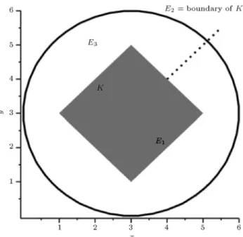
Example 3.2. Let U = fx = (x1; x2) 2 R2 j (x1
3)2+(x2 3)2 9g, and let K be a polytope generated
by the following closed half-spaces: g1(x) = x1+ x2 8 0;
g2(x) = x1 x2 2 0;
g3(x) = x1+ x2 4 0;
g4(x) = x1 x2+ 2 0:
Suppose that E is an equivalence relation on U such that U=E = fE1; E2; E3g where:
E1= fx 2 U : x is an interior point of polytope Kg;
E2= fx 2 U : x is a boundary point of polytope Kg;
E3= fx 2 U : x is an exterior point of polytope Kg:
Now, assume that M is a rough feasible region in the approximation space A = (U; E) such that M =
E1 [ E2 and M = E1 [ E2 [ E3 are lower and
upper approximations of M, respectively. Also, the boundary of M is given by MBN = E3 (see Figure 1).
The structure of M is taken from [7,6]. Consider the following RMOP problem:
max f1(x) = (x1 4)2+ (x2 2)2 2
max f2(x) = x21+ x22 5x1x2
max f3(x) = 5 (x1 1)2 (x2 3)2
s:t: x 2 M
M M M: (11)
In order to nd some ecient solutions to Problem (11), we solve some crisp SOP problems by Theorems 3.1-3.5.
Figure 1. The set K and equivalence classes of E on U. First step: Finding the rough optimal value f = ( f1; f2; f3):
f1= a1= f1(1; 3) = f1(3; 5) = 8;
f1= c1= f1(0:8787; 5:1213) = 17:4853;
f2= a2= f2(1; 3) = f2(3; 1) = 5;
f2= c2= f2(4:0209; 0:1791) = 12:6;
f3= f3= a3= f3(1; 3) = 5 c3= f3(1 ; 3 )
= 5 < a3:
Second step: Finding the rough optimal sets for any objective function:
F O1
ss = fx 2 Mj f1(x) = f1= 17:4853g = ;;
F O1
sp= fx 2 Mj f1(x) f1= 8g = f(1; 3); (3; 5)g;
F O1
ps= fx 2 Mj f1(x) = f1= 17:4853g
= f(0:8787; 5:1213)g; F O1
pp = fx 2 Mj f1(x) f1= 8g
= f(x1; x2) 2 U : (x1 4)2+ (x2 2)2 10g;
F O2
ss = fx 2 Mj f2(x) = f2= 12:6g = ;;
F O2
F O2ps= fx 2 Mj f
2(x) = f2 = 12:6g
= f(4:0209; 0:1791)g; F O2pp= fx 2 Mj f
2(x) f2= 5g
= f(x1; x2) 2 U : x21+ x22 5x1x2 5g:
Finally, since c3 < a3, F O3ss = F O3sp = F O3ps =
F O3
pp = f(1; 3)g.
Third step: Finding the rough completely optimal sets:
F Os(sc)= 3
\
j=1
F Ojss = ;;
F Os(pc) = 3
\
j=1
F Ojsp= f(1; 3)g;
F Op(sc) = 3
\
j=1
F Oj ps= ;;
F Op(pc)= 3
\
j=1
F Oj
pp= f(1; 3)g:
Therefore, Problem (11) has no surely-complete opti-mal solution. But, the point x = (1; 3) is a
possibly-complete optimal solution.
Fourth step: Finding the rough ecient solutions sets, rstly, the sets P; Q; S, and T are as follows:
P = [3
j=1
F Oj
ss= f(1; 3)g;
Q =[3
j=1
F Oj
sp= f(1; 3); (3; 5); (3; 1)g;
S =
3
[
j=1
F Ojps=f(0:8787; 5:1213);(4:0209; 0:1791);(1; 3)g;
T =
3
[
j=1
F Ojpp=x 2 U : f(x1 4)2+(x2 2)2 10g
[ fx2
1+ x22 5x1x2 5g :
Secondly, according to Theorems 3.2-3.5, we solve the SOP problems P 1; P 2; P 3; and P 4 as follows:
P 1 :
max w1 (x1 4)2+ (x2 2)2 2
+ w2 x21+ x22 5x1x2
+ w3 5 (x1 1)2 (x2 3)2
s:t: x1+ x2 8 0
x1 x2 2 0
x1+ x2 4 0
x1 x2+ 2 0
fr(x) = fr;
where r 2 f1; 2; 3g. P 2 :
max w1 (x1 4)2+ (x2 2)2 2
+ w2 x21+ x22 5x1x2+
w3 5 (x1 1)2 (x2 3)2
s:t: x1+ x2 8 0
x1 x2 2 0
x1+ x2 4 0
x1 x2+ 2 0
fr(x) fr;
where r 2 f1; 2; 3g. P 3 :
max w1 (x1 4)2+ (x2 2)2 2
+ w2 x21+ x22 5x1x2+
w3 5 (x1 1)2 (x2 3)2
s:t: (x1 3)2+ (x2 3)2 9
fr(x) = fr;
where r 2 f1; 2; 3g. P 4 :
max w1 (x1 4)2+ (x2 2)2 2
+ w2 x21+ x22 5x1x2+
w3 5 (x1 1)2 (x2 3)2
s:t: (x1 3)2+ (x2 3)2 9
where r 2 f1; 2; 3g.
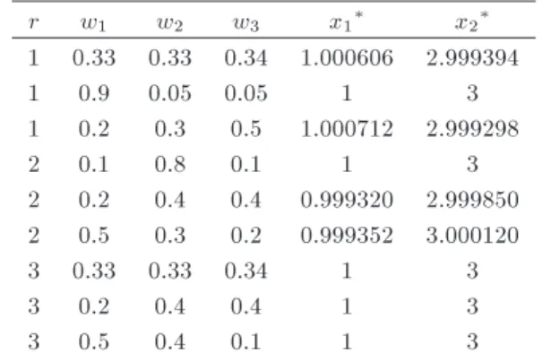
By changing the weights, we can get dierent ecient solutions, which are handled by the DM (see Tables 1-4).
In Table 1, since there is no ^x 2 M such that
Table 1. Surely-feasible, and surely-ecient solutions with dierent weights to Problem P 1.
r w1 w2 w3 x1 x2
3 0.33 0.33 0.34 1.000606 2.999394 3 0.1 0.1 0.8 1.000577 2.999423 3 0.5 0.4 0.1 1.000580 2.99910 Table 2. Surely-feasible and possibly-ecient solutions with dierent weights to Problem P 2.
r w1 w2 w3 x1 x2
1 0.33 0.33 0.34 1.000606 2.999394
1 0.9 0.05 0.05 1 3
1 0.2 0.3 0.5 1.000712 2.999298
2 0.1 0.8 0.1 1 3
2 0.2 0.4 0.4 0.999320 2.999850 2 0.5 0.3 0.2 0.999352 3.000120
3 0.33 0.33 0.34 1 3
3 0.2 0.4 0.4 1 3
3 0.5 0.4 0.1 1 3
Table 3. Possibly-feasible and surely-ecient solutions with dierent weights to Problem P 3.
r w1 w2 w3 x1 x2
1 0.33 0.33 0.34 0.8786796 5.121320 1 0.8 0.1 0.1 0.8691861 5.111786 1 0.4 0.5 0.1 0.8614629 5.103963 2 0.4 0.5 0.1 4.019090 0.1783941 2 0.7 0.2 0.1 4.019602 0.1785793 2 0.1 0.3 0.6 4.019006 0.1783636 3 0.33 0.33 0.34 0.9995549 2.999893 3 0.2 0.4 0.4 0.9990667 3.000117 3 0.5 0.4 0.1 0.9992445 2.999690 Table 4. Possibly-feasible and possibly-ecient solutions with dierent weights to Problem P 4.
r w1 w2 w3 x1 x2
1 0.33 0.33 0.34 0.1724377 4.002443 1 0.2 0.4 0.4 0.1534008 3.947034 1 0.5 0.4 0.1 0.2214822 4.131300 2 0.33 0.33 0.34 0.1724377 4.002443 2 0.2 0.4 0.4 0.1534008 3.947034 2 0.1 0.3 0.6 0.1119307 3.811823 3 0.33 0.33 0.34 0.9996620 3.000140 3 0.2 0.4 0.4 0.9995774 2.999938 3 0.5 0.4 0.1 0.9996227 2.999917
fr(^x) = fr for r = 1; 2, the results are provided only
for r = 3.
Table 2, for all r = 1; 2; 3, gives the point x =
(1; 3) as a surely-feasible and possibly-ecient solution. Table 3 presents dierent points of the set S which are possibly-feasible and surely-ecient solutions. Finally, in Table 4, all of the obtained solutions are possibly-feasible and possibly-ecient, which belong to the set T .
Example 3.3. Consider Example 3.2 where the third objective function is changed as follows:
max f3(x) = 2x31x2 2x1x32:
Then, f3 = a3 = f3(5; 3) = 480, f3 = c3 =
f3(5:99; 3:2445) = 985:4736; and the rough optimal sets
for the function f3are:
F O3
ss = fx 2 Mj f3(x) = f3= 985:4736g = ;;
F O3sp= fx 2 Mj f3(x) f3= 480g = f(5; 3)g;
F O3
ps= fx 2 Mj f3(x) = f3= 985:4736g
= f(5:99; 3:2445)g; F O3pp = fx 2 Mj f
3(x) f3= 480g
= f(x1; x2) 2 U : 2x31x2 2x1x32 480g:
Hence, the rough completely optimal sets are: F Os(sc)= F Os(pc)= F Op(sc) = ;;
F Op(pc)=
x 2 U : fx1 4)2+ (x2 2)2 10g
\ fx2
1+ x22 5x1x2 5g
\ f2x3
1x2 2x1x32 480g
:
So, Problem (11) with the new objective function f3 has neither surely-complete optimal solution nor
surely-feasible and possibly-complete optimal solution. At the last step, for obtaining the rough ecient solutions sets we need to nd the sets P; Q; S; and T as follows:
P = [3
j=1
F Oj ss= ;;
Q = [3
j=1
F Oj
S =[3
j=1
F Oj
ps= f(0:8787; 5:1213); (4:0209; 0:1791);
(5:99; 3:2445)g; T =[3
j=1
F Oj pp=
x 2 U : f(x1 4)2+ (x2 2)2 10g
[ fx2
1+ x22 5x1x2 5g
[ f2x3
1x2 2x1x32 480g
:
P = ; means that there is no ^x 2 Msuch that fr(^x) =
fr for r = 1; 2; 3. Thus, Problem P 1 (by replacement
of the new objective function f3) is infeasible and there
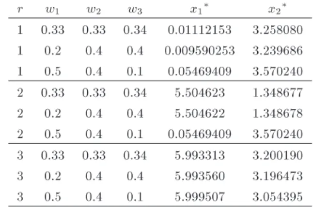
is no surely-feasible and surely-ecient solution. For nding ecient solutions of other degrees, see Tables 5, 6, and 7.
Example 3.4. Let U = fx = (x1; x2) 2 R2 j 3
x1 3; 3 x2 3g.
Suppose that E is an equivalence relation on U such that it generates a partition as U=E = fEij j
Table 5. Surely-feasible and possibly-ecient solutions with dierent weights to Problem P 2.
r w1 w2 w3 x1 x2
1 0.33 0.33 0.34 1 3
1 0.1 0.8 0.1 3 5
1 0.7 0.1 0.2 1.000606 2.999394
2 0.1 0.8 0.1 1 3
2 0.2 0.4 0.4 1.00022 2.99911 2 0.5 0.4 0.1 0.999105 3.000114 3 0.33 0.33 0.34 5.000001 3.000001
3 0.2 0.4 0.4 5 3
3 0.5 0.4 0.1 5 2.999999
Table 6. Possibly-feasible and surely-ecient solutions with dierent weights to Problem P 3.
r w1 w2 w3 x1 x2
1 0.33 0.33 0.34 0.8786796 5.121320 1 0.2 0.4 0.4 0.8786750 5.121532 1 0.7 0.15 0.15 0.881485 5.100560 2 0.33 0.33 0.34 4.023270 0.1799071 2 0.2 0.4 0.4 4.023233 0.1798934 2 0.5 0.4 0.1 4.023014 0.1798143 3 0.33 0.33 0.34 5.990152 3.242885 3 0.2 0.4 0.4 5.990023 3.244462 3 0.7 0.15 0.15 5.990024 3.244446
Table 7. Possibly-feasible and possibly-ecient solutions with dierent weights to Problem P 4.
r w1 w2 w3 x1 x2
1 0.33 0.33 0.34 0.01112153 3.258080 1 0.2 0.4 0.4 0.009590253 3.239686 1 0.5 0.4 0.1 0.05469409 3.570240 2 0.33 0.33 0.34 5.504623 1.348677 2 0.2 0.4 0.4 5.504622 1.348678 2 0.5 0.4 0.1 0.05469409 3.570240 3 0.33 0.33 0.34 5.993313 3.200190 3 0.2 0.4 0.4 5.993560 3.196473 3 0.5 0.4 0.1 5.999507 3.054395 i; j = 1; :::; 6g where:
Eij=fx 2 U j j 1 x1 j 3;
3 i x2 4 ig for all i; j = 1; :::; 6:
Now, assume that M is a rough feasible region in the approximation space A = (U; E) such that the lower and upper approximations of M are as follow:
M= f(x1; x2) 2 U j 1 x1 1; 1 x2 1g;
M= f(x
1; x2) 2 U j 2 x1 2; 2 x2 2g:
Also, the boundary region of M is given by:
MBN =f(x1; x2) 2 U j 2 x1< 1; 1 < x1 2;
2 x2< 1; 1 < x2 2g;
(see Figure 2). We consider the following RMOP problem:
max f1(x) = x21+ (x2 1)2
max f2(x) =p2x1x2+ 5 x32
max f3(x) = 2x1x2 x21
s:t: x 2 M
M M M: (12)
To nd the solutions of Problem (12), similar to Example 3.2, we proceed as follow:
First step: Finding the rough optimal value f = ( f1; f2; f3):
f1= a1= f1( 1; 1) = f1(1; 1) = 5;
f1= c1= f1( 2; 2) = f1(2; 2) = 13;
f2= a2= f2( 1; 1) =
p 7 + 1;
f2= c2= f2( 2; 2) =p13 + 8;
f3= a3= f3( 1; 1) = f3( 1; 1) = 1;
f3= c3= f3(2; 2) = f3( 2; 2) = 4:
Second step: Finding the rough optimal sets for any objective function:
F O1ss = fx 2 Mj f1(x) = f1= 13g = ;;
F O1
sp= fx 2 Mj f1(x) f1= 5g
= f( 1; 1); (1; 1)g; F O1
ps= fx 2 Mj f1(x) = f1= 13g
= f( 2; 2); (2; 2)g; F O1
pp = fx 2 Mj f1(x) f1= 5g
= f(x1; x2) 2 U : x21+ (x2 1)2 5g;
F O2
ss = fx 2 Mj f2(x) = f2=
p
13 + 8g = ;; F O2
sp= fx 2 Mj f2(x) f2=
p 7 + 1g = f( 1; 1)g;
F O2
ps= fx 2 Mj f2(x) = f2=
p 13 + 8g = f( 2; 2)g;
F O2
pp = fx 2 Mj f2(x) f2g
= f(x1; x2) 2 U :p2x1x2+ 5 x32
p 7 + 1g;
F O3
ss = fx 2 Mj f3(x) = f3= 4g = ;;
F O3sp= fx 2 Mj f3(x) f3= 1g
= f( 1; 1); (1; 1)g; F O3
ps= fx 2 Mj f3(x) = f3= 4g
= f( 2; 2); (2; 2)g; F O3
pp = fx 2 Mj f3(x) f3= 1g
= f(x1; x2) 2 U : 2x1x2 x21 1g:
Third step: Finding the rough completely optimal sets:
F Os(sc)= 3
\
j=1
F Ojss= ;;
F Os(pc) = 3
\
j=1
F Oj
sp= f( 1; 1)g;
F Op(sc) = 3
\
j=1
F Oj
ps= f( 2; 2)g;
F Op(pc)=
x 2 U : fx2
1+ (x2 1)2 5g
\ fp2x1x2+ 5 x32
p 7 + 1g \ f2x1x2 x21 1g
:
Therefore, Problem (12) has no surely-feasible and surely-complete optimal solution. But, the point x =
( 1; 1) is a surely-feasible and possibly-complete optimal solution and x = ( 2; 2) is a possibly-feasible and surely-complete optimal solution.
Fourth step: Finding the rough ecient solutions set, rstly, the sets P , Q, S, and T are as follow:
P =
3
[
j=1
F Oj ss= ;;
Q =
3
[
j=1
F Oj
sp= f( 1; 1); (1; 1); (1; 1)g;
S = [3
j=1
F Oj
ps= f( 2; 2); (2; 2); (2; 2)g;
T = [3
j=1
F Oj pp =
x 2 U : fx2
[ fp2x1x2+ 5 x32
p 7 + 1g [ f2x1x2 x21 1g :
Secondly, according to Theorems 3.2-3.5, we need to solve the SOP problems Q1, Q2, Q3 and Q4 with dierent weights.
Q1 :
max w1 x21+ (x2 1)2
+ w2 p2x1x2+ 5 x32
+w3 2x1x2 x21
s:t: 1 x1 1
1 x2 1
fr(x) = fr;
where r 2 f1; 2; 3g. Q2 :
max w1 x21+ (x2 1)2
+ w2 p2x1x2+ 5 x32
+ w3 2x1x2 x21
s:t: 1 x1 1
1 x2 1
fr(x) fr;
where r 2 f1; 2; 3g. Q3 :
max w1 x21+ (x2 1)2
+ w2 p2x1x2+ 5 x32
+ w3 2x1x2 x21
s:t: 2 x1 2
2 x2 2
fr(x) = fr;
where r 2 f1; 2; 3g. Q4 :
max w1 x21+ (x2 1)2
+ w2 p2x1x2+ 5 x32
+ w3 2x1x2 x21
s:t: 2 x1 2
2 x2 2
fr(x) fr;
where r 2 f1; 2; 3g.
Therefore, we can get the rough ecient solutions sets of dierent degrees. Since P = ;, there is no ^x 2 M such that fr(^x) = fr for r = 1; 2; 3. Thus,
Problem Q1 is infeasible and there is no surely-feasible and surely-ecient solution. But, for nding ecient solutions of other degrees, the rest of calculations are similar to those of Examples 3.2 and 3.3.
Remark 3.3. Note that it is possible that some of the sets P; Q; S; and T be empty. In this case, further research is needed to nd surely- and possibly-ecient solutions to RMOP problems.
4. Conclusion
In this paper, we rst reviewed the basic concepts of rough set theory and recalled some preliminary concepts and results of the kinds of solutions of a multi-objective programming problem by paying special at-tention to a scalarization method used to obtain a so-lution. We also reviewed rough programming problems and introduced the concept of Rough Multi-Objective Programming (RMOP) problems. Then RMOP prob-lems were classied into ve classes. We have just proposed a method for obtaining the solutions of the rst class, where the feasible region is a rough set, while all the objective functions are crisp. In this regard, we discussed new concepts such as \surely-complete opti-mal solutions", \possibly-complete optiopti-mal solutions", \surely-ecient solutions" and \possibly-ecient solu-tions". Also, we solved some numerical examples for illustration.
Extending our study to the remaining four other classes is a subject for future research. Application of our methods to real-world problems may also lead to further considerations.
Acknowledgments
The authors would like to express their gratitude to the anonymous reviewers for the comments and suggestions, which greatly helped them to improve the paper.
References
1. Ehrgott, M., Multicriteria Optimization, 2nd Ed., Springer, Berlin (2005).
2. Pawlak, Z. \Rough sets", International Journal of Information and Computer Sciences, 11(5), pp. 341-356 (1982).
3. Liu, B. \Theory and practice of uncertain program-ming", Physica Verlag, New York (2002).
4. Xu, J. and Tao, Z., Rough Multiple Objective Decision Making, CRC Press, New York (2011).
5. Hamzehee, A., Yaghoobi, M.A. and Mashinchi, M. \Linear programming with rough interval coecients", Journal of Intelligent and Fuzzy Systems, 26, pp. 1179-1189 (2014).
6. Youness, E.A. \Characterizing solutions of rough pro-gramming problems", European Journal of Operational Research, 168(3), pp. 1019-1029 (2006).
7. Osman, M.S., Lashein, E.F., Youness, E.A. and At-teya, T.E.M. \Mathematical programming in rough environment", Optimization, 60(5), pp. 603-611 (2011).
8. Sakawa, M. \Fuzzy sets and interactive multiobjective optimization", Plenum Press, New York and London (1993).
9. Greco, S., Matarazzo, B. and Slowinski, R. \Rough set theory for multicriteria decision analysis", European Journal of Operational Research, 129(1), pp. 1-47 (2001).
10. Xu, J. and Zhao, L. \A class of fuzzy rough expected value multi-objective decision making model and its application to inventory problems", Computers and Mathematics with Applications, 56(8), pp. 2107-2119 (2008).
11. Xu, J. and Zhao, L. \A multi-objective decision-making model with fuzzy rough coecients and its application to the inventory problem", Information Sciences, 180(5), pp. 679-696 (2010).
12. Xu, J. and Yao, L. \A class of multiobjective linear programming models with random rough coecients", Mathematical and Computer Modelling, 49(1-2), pp. 189-206 (2009).
13. Xu, J. and Yao, L. \A class of expected value multi-objective programming problems with random rough coecients", Mathematical and Computer Modelling, 50(1-2), pp. 141-158 (2009).
14. Xu, J., Li, B. and Wu, D. \Rough data envelopment analysis and its application to supply chain perfor-mance evaluation", International Journal of Produc-tion Economics, 122(2), pp. 628-638 (2009).
15. Tao, Z. and Xu, J. \A class of rough multiple objective programming and its application to solid transporta-tion problem", Informatransporta-tion Sciences, 188, pp. 215-235 (2012).
16. Li, F., Jing, Y., Shi, Y. and Jin, C. \Research on the theory and method of rough programming based on synthesis eect", International Journal of Innovative Computing, Information and Control, 9(5), pp. 2087-2098 (2013).
17. Li, F., Jin, C., Jing, Y., Wilamowska-Korsak, M. and Bi, Z. \A rough programming model based on the greatest compatible classes and synthesis eect", Systems Research and Behavioral Science, 30(3), pp. 229-243 (2013).
18. Pawlak, Z. \Rough sets, rough relations and rough functions", Fundamental Informaticae, 27, pp. 103-108 (1996).
Biographies
Ali Hamzehee was born in 1974 in Iran. He received his BS and MS degrees both in Applied Mathematics from Vali Asr University of Rafsanjan and Amir Kabir University of Tehran, in 1997 and 1999, respectively. He is currently a PhD student in Department of Mathematics, Faculty of Mathematics and Computer, Shahid Bahonar University of Kerman. Currently, he is a Lecturer at the Department of Mathematics in Islamic Azad University, Kerman Branch. His research interests include operational research, decision making, fuzzy programming and rough programming.
Mohammad Ali Yaghoobi is Assistant Professor in the Mathematics Department at the Shahid Bahonar University of Kerman (SBUK), Iran, where he was the Head of Statistics Department from December 2006 to March 2009. He received his MS degree, ranked rst, in Applied Mathematics and his PhD degree in the same eld in branch of Operational Research from the SBUK. His main research interests are in the elds of multiple criteria decision making, goal programming, fractional programming, linear and integer programming, and fuzzy programming. He has published several papers in national and international journals.
Mashaallah Mashinchi was born in 1951 in Iran. He received his BS and MS degrees both in Statistics, from Ferdowsi University of Mashhad and Shiraz University, in 1976 and 1978, respectively, and his PhD degree in Mathematics from Waseda University in Japan, in 1987. He is now a Professor in the Department of Statistics at Shahid Bahonar University of Kerman (SBUK), Iran. He is also Editor-in-Chief of the Iranian Journal of Fuzzy Systems, and the Director of the Fuzzy Systems & Applications Center of Excellence at SUBK. His current research interests include fuzzy mathematics, especially in statistics, decision making and algebraic systems.