Sharif University of Technology
Scientia IranicaTransactions B: Mechanical Engineering www.scientiairanica.com
A fast face detection method for illumination variant
condition
C.-H. Hsia
a, J.-S. Chiang
b;and C.-Y. Lin
ba. Department of Electrical Engineering, Chinese Culture University, Taipei, Taiwan. b. Department of Electrical Engineering, Tamkang University, New Taipei, Taiwan. Received 22 May 2014; received in revised form 1 April 2015; accepted 4 May 2015
KEYWORDS Illumination variant face detection; Adaboost; Neural network; Modied census transform;
Real-time detection.
Abstract. General boosting algorithms for face detection use rectangular features. To obtain a better performance, it needs more training samples and may generate an unpredictable number of features. Besides using pixel values, which are easily aected by illumination, to calculate the rectangular features, it usually needs to preprocess the data before calculating the values of the features. Such an approach may increase computation time. To overcome the drawbacks, we propose a new solution based on the Adaboost algorithm and the Back Propagation Network (BPN) of a Neural Network (NN), combining local and global features with cascade architecture to detect human faces. We use the Modied Census Transform (MCT) feature, which belongs to texture features and is less sensitive to illumination, for local feature calculation. In this approach, it is not necessary to preprocess each sub-window of the image. For classication, we use the structure of the hierarchical feature to control the number of features. With only MCT, it is easy to misjudge faces and, therefore, in this work, we include the brightness information of global features to eliminate the False Positive (FP) regions. As a result, the proposed approach can have a Detection Rate (DR) of 99%, an FPs of only 11, and detection speed of 27.92 Frames Per Second (FPS).
© 2015 Sharif University of Technology. All rights reserved.
1. Introduction
Face detection is one of the most important factors in face recognition. A good face detection method must be able to detect the human face eectively with the requirement of a higher Detection Rate (DR), a lower False Positive Rate (FPR), and real-time processing capabilities. The features of gestures and expressions of a face, the light source, shelter, a beard, etc. may aect the detection performance in the face recognition system.
In recent years, the most successful approach to
*. Corresponding author. Tel.: +886-2-2621-5656#3055; Fax: +886-2-2620-9814
E-mail addresses: [email protected] (C.-H. Hsia); [email protected] (J.-S. Chiang)
face detection is extracting the outlook characteristics of an image, such as edge, grayscale intensity and color, and, then, through machine learning, it can recognize the human face. Real-time face detection was rst proposed by Viola and Jones [1,2]. They used rectangular features to train the classier in face detection, and it has become one of the most successful algorithms for frontal face detection. However, detec-tion speed is aected by the number of weak classiers and the complexity of preprocessing. Ali et al. [3] proposed an approach combining pose-indexed features and pose estimators with the Adaboost algorithm to detect human faces. It can select and combine posture assessment in the learning process to eliminate the impact of dierent attitudes. This method can improve the shortcomings of the original Adaboost algorithm which only detects the frontal face. However, this
approach is still Adaboost algorithm-based, and de-tection speed decreases upon increasing the number of weak classiers. The conventional Adaboost algorithm focuses on detection performance, but it needs to be adjusted in practical applications. It has to consider the cost of misclassication, and a cost-sensitive boost-ing algorithm is, thus, proposed to solve this problem. Researchers in [4] improved the cost-sensitive boosting algorithm by changing the sample error and updating the weights and thresholds to calculate the real costs incurred due to incorrect classication. Wang et al. [5] also added the feature to de-select the irrelevant weak classiers. Shen et al. [6] used Boosted Greedy Sparse Linear Discriminant Analysis (BGSLDA) to train the rectangular features to nd the weak classiers in order to maximize separation between dierent classes. Shih and Lin [7] used Discriminating Features Analysis (DFA), and, by combining the Support Vector Machine (SVM), to detect human faces. DFA can help to produce an eective feature. Guo et al. [8] used the methods of probability-based face mask pre-ltering and pixel-based hierarchical feature Adaboosting to solve the drawbacks of the computational complexity of the issue of the original Adaboost algorithm. In this approach, it uses Histogram Equalization (HE) for pre-processing before using a mask or hierarchical feature to improve the brightness distribution. However, HE requires considerable computation time. According to the experiment, if it uses HE for pre-processing the resolution of a 320 240 image with a search window of 2424 in size, it needs a total of 81,451 sub-windows, and takes 342 ms computation time (with a single 2.4 GHz CPU). The skin color of the human face is an important feature, and its detection can be used for various applications. Gihimire and Lee [9] proposed a face detection method based on skin color and the edge of the color image. This approach enhances the color image in the HSV space, and segments the skin color in the YCbCr and RGB spaces. Finally, it is combined with the edges of the color image. By using the histogram skin color model in the HS color space, Liu and Peng [10] segmented skin color by the histogram back projection approach. Then, they used morphological and blob analyses to rene the segmentation result with optimization. Powar and Jahagirdar [11] adopted the, so called, \reference white" to realize light compensation and detect the candidate face region by the YCbCr skin color model. They used the morphological operations and Adaboost algorithm to accomplish accurate face detection. Wang and Xia [12] used the YCbCr skin color model to detect the potential face regions. They also detected lips, eyes, and ellipse shapes to verify these potential facial regions. Ng and Pun [13] performed face detection to nd the face position rst. They then classied the skin pixels to generate a skin probability map
to form the skin mask for skin segmentation. Tan et al. [14] used the face skin color for face tracking, gesture analysis, and human{computer interaction. However, skin color is susceptible to the inuence of dierent lighting conditions, and even in dierent color spaces, it may also cause misjudgment. Liu et al. [15] proposed an approach for skin color detection under rapidly changing lighting conditions. They rst detect illumination changing. If the illumination has not changed, it classies the skin color under the same illumination condition. If the illumination has changed, it processes the face detection and color correction to record the current illumination conditions for the next image frame. Due to massive computation time, detection speed is less than 5 FPS. Researchers in [16] proposed a GPU-based face detection (to accelerate object detection in images and video sequences using graphics processors), based on local rank patterns, as an alternative to the commonly used Haar wavelets. Moreover, recent work [17,18] dealt with the face detection of emotions or expression recognition by employing visual sensors.
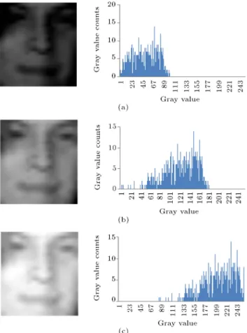
Light illumination is a very important issue for human face detection. Figure 1 shows images with
Figure 1. Face illumination distribution statistics: (a) A low brightness image and its grayscale histogram; (b) a normal brightness image and its grayscale histogram; and (c) a high brightness image and its grayscale histogram.
Figure 2. Cascaded classier architecture.
grayscale value distribution of a face under dierent brightness. We can use the technique of HE to adjust too dark or too bright images. The rectangular features calculated from grayscale values are easily aected by illumination, and normalization can reduce illumination eects [2]. The approach proposed in [2] calculates the standard deviation of the sub-window after calculating the feature value, and, then, it is used for normalization to reduce the impact of dierent illu-mination conditions. Since the normalization for each feature needs two integral images, it will increase the computation complexity. Generally speaking, process-ing for face detection would take a lot of computation time.
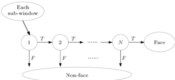
2. Traditional cascade classier architecture If classication uses a single strong classier, it may need more computation time. Because it calculates a large number of rectangular features, it will judge the target after calculation. The cascaded architecture proposed by Viola and Jones [2] is shown in Figure 2.
The one-stage cascaded classier architecture uses several weak classiers by voting to decide faces. The rst stage classier uses less rectangular features, but can eliminate most non-face sub-windows. The latter stages need more weak classiers to calculate the rectangular features to eliminate remaining non-face sub-windows. The FPR can be calculated as:
FPR =YK
i=1
fi: (1)
And DR can be calculated as: DR =
K
Y
i=1
di; (2)
where K denotes the number of stages, fithe ithFPR,
and di the ithDR. Details of the cascade architecture
algorithm are described as follows:
Algorithm 1. Traditional cascade architecture algo-rithm:
1. Set a maximum acceptable FPR f and a minimum acceptable detection rate, d;
2. Set the target false positive rate, Ftarget;
3. P = positive samples;
4. N = negative samples;
5. Initialize FPR (F0= 1:0) and DR (D0= 1:0);
6. i = 0;
7. While Fi> Ftarget;
8. i = i + 1;
9. ni= 0; Fi= Fi 1;
10. While Fi> f Fi 1;
11. ni= ni+ 1;
12. Use P and N to train a classier with ni features;
13. Calculate the current Fi and Di;
14. Decrease the threshold for the ithclassier until the
current cascade classier has a detection rate of at least d Di 1 (this also aects Fi);
15. N = 0 (clear all negative samples and add misclas-sication negative samples as the next step);
16. If Fi > Ftarget, then add misclassication of the
non-face samples to N.
It sends the misclassied non-face negative samples (maximum FPR is 50% of the previous N set in this study) to the next stage for training. From this approach, in order to classify the non-face samples from the previous stages, it needs more rectangular features for classication. Therefore, if the training samples are large and complex, the cascade architecture for training will get more rectangular features and stages. Although the rst few stages can rule out non-face sub-windows quickly, more time is needed for face judgment in the latter stages.
3. New illumination variant face detection method
According to the cascade classier architecture de-scribed in the previous section, the number of rect-angular features is unknown for face judging, and it depends on the number of negative samples and the degree of diculty of the classication. With more quantities, more time may be needed for calculation without a limit number. Therefore, this work tries to use the concept of hierarchies that will control the number of features, such that it can reduce a lot of computation time. For the illumination is-sue, the texture feature has less sensitivity to light illumination, and will be discussed in the following subsections.
3.1. Modied census transform
In this study, the Census Transform (CT) is replaced by the Modied Census Transform (MCT) [19] for calculation. In order to improve the discrimination of CT [20], it describes the texture information in the interested region. It also has the characteristics of simpler operation and less sensitivity to illumination:
C(x) = y2N(I(x); I(x0)); (3)
where (I(x); I(x0)) is a comparison function to
com-pare the values of I(x) with that of I(x0). If I(x0) >
I(x), then the result is 1, otherwise 0. x denotes the center pixel, and x0 denotes the set of surrounding
pixels around the center point. On a 3 3 window neighborhood, the total surrounding pixels are 8 points (set N). Operator denotes the concatenation oper-ation that concatenates all these binary values. It is Z-shaped in this case.
By adding the comparisons of the center pixel and setting the mean value as the threshold, it improves the discriminative capability of CT, as follows:
(x) = y2N0 I(x); I(x0); (4)
where I(x) is the mean value that includes the center pixel and surrounding pixels, and set N0 contains the
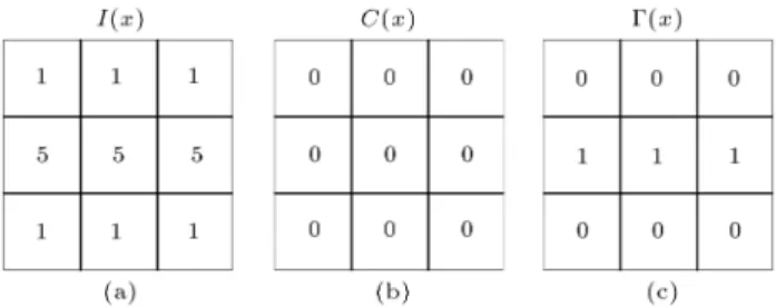
center pixel and surrounding pixels. As mentioned in [19], with the grayscale intensity as shown in the following situation of Figure 3, CT cannot describe the texture information exactly.
Let us analyze the illumination impact for texture features by a simple image formation model, as follows:
I(x) = gL(x)R(x) + b; (5)
where x denotes the position of the image, I(x) the image intensity, L(x) the luminance, R(x) the object reectance, g the gain factor of the camera, and b a bias, which is assumed to be a constant in the image plane. It does not usually have unique solutions for gL(x) and R(x) when calculating an image plane and is called an ill-posed problem. It usually assumes that L(x) varies slowly and smoothly at point x. Based on this assumption, the impact factor of illumination is a constant, L(x) = L, and, therefore, I(x) only changes
Figure 3. CT and MCT coding: (a) Grayscale values in a 33 window; (b) using CT; and (c) using MCT.
Figure 4. Dierent illumination images and their corresponding grayscale values of CTs coding: (a) Low brightness; (b) normal brightness; (c) high brightness; (d) the grayscale value of CT coding for (a); (e) the grayscale value of CT coding for (b); and (f) the grayscale value of CT coding for (c).
with R(x) linearly. For this kind of texture feature, the illumination eect is eliminated, and is less sensitive to illumination. Figure 4 shows the grayscale images of CT coding obtained with dierent illuminations. It is found that no matter the conditions of illumination, feature coding is quite similar; it explains that texture features are less sensitive to illumination.
3.2. Global binary pattern
For the texture features of the above discussion, the brightness information in the feature coding process can be removed. However, darker eyes and brighter cheeks cannot be considered. Therefore, we add the brightness characteristics of the face to compensate for the brightness information of texture features that were removed.
Considering real-time operation, we use a simple method to calculate the brightness information. Con-sidering an image block n n in size (letting m = n2)
and X1; X2; , and Xm are grayscale values of the
block. Then:
X = m1 Xm
i=1
Xi; (6)
where X is the mean value of the block. Let us set
X as the threshold value, Xth. It then compares Xth
with all pixels in the image block to calculate the brightness information and will generate the Global Binary Pattern (GBP) as follows:
outputi= (
1; Xi> Xth
0; otherwise (7)
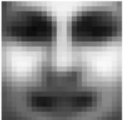
Figure 5. Brightness information of the probability distribution map of the face samples.
samples, count the probability of 1 or 0 appearing in every pixel and normalize it to a grayscale image. The part with more brightness has higher probability of 1 appearing, namely, the bright part of the human face, and vice versa for less brightness. Before using this information for training and testing, the HE must be used for processing to increase the contrast of the eyes and cheeks when the background is dark or light, and further to reduce FP detection.
3.3. The proposed Adaboost algorithm
In this work, we use the Adaboost algorithm for human face detection. The algorithm is described as follows: Algorithm 2. Adaboost strong classier algorithm:
1. Given the training set ( 1; c1); ; ( m; cm), where
m denotes the total number of samples, ithe input
sample, and ci = 0 or 1, the positive or negative
samples.
2. Initialize sample weighting D1(i) = 2l1 (l denotes
the number of positive samples) or 1
2n (n denotes
the number of negative samples).
3. For t = 1 K (K denotes the iteration).
4. Find the best weak classier (the weak classier algorithm is described in the following sub-section).
5. t=12ln
1 "t
"t
, where tis the weight coecient.
6. Update weighted distribution: Dt+1(i) = DZt(i)
t
(
e t if !
t( i(x)) = ci
et if !t( i(x)) 6= ci
where Zt=Pmi=1Dt(i) and !t( i(x))i is a look-up
table for a weak classier.
7. Build the elementary classier of a single feature position, x:
hx() = K
X
t=1
twt()I(x = xt);
where is the MCT feature.
Figure 6. Black point represents the best weak classier. Table 1. Texture features and their weighted values. Texture feature 0 248 510 Weighted value 43832 18517 43832
8. Construct a strong classier architecture: H( ) =X
x
hx( (x)):
9. Find the single weak classier threshold, Tx:
Tx= 12 K
X
t=1
tI(x = xt):
3.4. The proposed weak classier algorithm Unlike the rectangle feature, every MCT represents the texture information at position (x; y) of the image that contains 511, (29 1), texture features [19]. All the
zeros and ones of the features are equal. Through the weak classier algorithm, it can nd not only the best weak classier, as shown in Figure 6, but also the weighted values corresponding to each texture feature for the best weak classier, as shown in Table 1.
It uses the lookup table technique to nd the weighted values corresponding to hx( (x)) and uses
Eq. (8) to calculate Hj( ). Finally, Hj( ) is compared
with threshold Tj (total of TX):
Hj( ) =
X
x2W0
hx( (x)); (8)
Hj( ) Tj; (9)
where x denotes the position of the weak classiers and W0 contains the weak classier set obtained from the
training process. If it is less than the threshold value, then it is passed to the next stage, otherwise, it is classied as non-face. In the training process, if DR is not 100%, it increases the threshold value until DR equals 100%. It usually occurs at the rst few stages, because there are not sucient numbers of features to classify positive and negative samples correctly.
Although adjustment of the threshold may have more non-face situations through the rst few stages, the subsequent stages can eliminate them eectively.
To learn a weak classier, it needs to count the MCT at every position of x rst, and then it compares g0
t with gt1 relating to the face or non-face situation.
Finally, it calculates the error, "t(x), and selects the
lowest error as the weak classier. Details of the weak classier algorithm [19] are described as follows: Algorithm 3. Weak classier algorithm:
1. Count MCT of positive and negative samples: g0
t(x; ) =
X
i;x;
Dt(i)I( i(x) = )I(ci = 0);
g1
t(x; ) =
X
i;x;
Dt(i)I( i(x) = )I(ci = 1);
where I() denotes a comparison function. If the condition in () is true, then, return to 1, otherwise, 0. Namely g0
t(x; ) is the MCT weighted value of
positive samples, and g1
t(x; ) is the MCT weighted
value of negative samples.
2. Calculate weighted error, "t, for each position, x:
"t(x) = "0t(x) + "1t(x);
"0 t(x) =
X
fg0
t(x; ) gt1(x; )g;
for positive samples, "1
t(x) =
X
fg0
t(x; ) > gt1(x; )g;
for negative samples.
3. Select the best feature of x (lowest error, "t):
xt= xj"t(x) = arg minf"t(x)g:
4. Create a look-up table for the weak classier: !t() =
(
0; if g0
t(xt; ) > gt1(xt; )
1; otherwise
3.5. Back propagation network algorithm The main theme of the Neural Network (NN) is to mimic biological NN learning and judgment. Biological neurons receive messages from a variety of sensors, and transmit them to nerve cells. By studying, analyzing, and summarizing these messages, it can achieve abili-ties of classication and judgment. In addition to the learning ability, it also has other advantages, such as:
1. High-speed computing power: Through parallel processing, it can rapidly nish calculations;
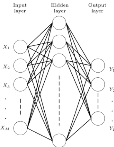
Figure 7. BPN contains an input layer, hidden layer, and output layer.
2. Fault tolerance: Because there are many links and nodes in the system, damage to a few links or nodes may not impair the overall performance signicantly.
The Back Propagation Network (BPN) is a supervised learning network that is particularly suitable for clas-sication and forecasting, like face detection, and the structure of BPN is shown in Figure 7.
The input layer, which looks like a sensory organ, can receive data into the system. The number of input nodes depends on the problem issues. In this study, because we use a sub-window, 2424 in size, the input layer has 576 nodes, and the GBP is used as the feature. It is not necessary for the hidden layer to be just a layer; it is possible to have no layer or more than one layer in the hidden layer part. A sucient number of nodes in the hidden layer reects the interaction between the input nodes. The hidden layer can increase the classication ability of the linear indivisible data. The output layer generates the output variables of the network. The numbers of nodes are decided according to the classication categories, and here, we use a node with an output value of approximately 1 for the face and of approximately 0 for a non-face.
There are two operation modes of BPN: the process of learning and the process of recalling. The process of learning sets the number of hidden layers, output layers, and nodes of each layer to determine the parameter values (linking, weighting, and threshold values) randomly. By sending the input training samples to this network, it constantly learns and corrects itself until reaching the set condition. The process of recalling can be nished through the training parameters for classication. The algorithm used in this work is the standard BPN algorithm.
3.6. The proposed face detection architecture When designing face detection architecture, it needs to consider both the accuracy and response time. Al-though the learning process of the Adaboost algorithm proposed in [2] using rectangular features is simple and fast, the trained cascade architecture often produces a lot of rectangular features and the massive rectangular features may take much time for face detection. For response time and performance consideration when using cascade architecture, it must limit the number of rectangular features.
For MCT in a 3 3 window size, the threshold value of MCT is the mean value of the sub-window. The coding sequence of MCT is in a Z-shaped direction. Figure 8 shows the coding for line and at features using the MCT method. Because the method using texture features only compares the values of the local area, the brightness information can be removed which can easily lead to false positives. The GBP technique can be used to calculate the brightness information of the facial feature to solve the FP problems.
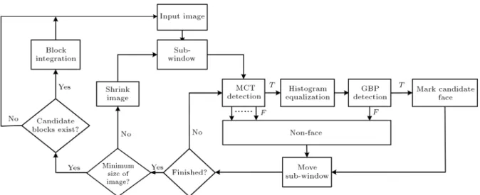
The proposed face detection architecture detects the face existing or not through a sub-window in the image, and the detection order is from left to right, top to bottom. Generally, the face may not be a xed sizein the image. If we want to detect dierent sizes
of faces, the image needs to be shrunk due to the xed size detection sub-window. In addition, through experiment, it can nd that there are overlaps near the face position for the possible candidate blocks due to the location being in the vicinity of the face. It needs to integrate these blocks for better judgment. The complete architecture is shown in Figure 9.
Generally speaking, using fewer weak classiers will lead to less computation time. The concept of hierarchical architecture would not only reduce com-putational complexity, but also would not impair the detection performance. We use a sub-window, 2424 in size, and the maximum number of calculation features is 22 22 = 484. The last stage is GBP, and it uses all the features of 576 points.
The rst (N 1) stages in the cascade architecture use the Adaboost algorithm to train the MCT, and the last stage uses BPN to train the GBP, as shown in Figure 10. Our architecture has two advantages:
1. Only one MCT feature value is calculated at each stage;
2. The computational complexity of the MCT feature is eased to have only one additional operation per MCT feature.
Unlike the traditional haar-like feature of Adaboost, it
Figure 8. Dierences of MCT: (a) Line feature; and (b) at feature.
Figure 10. Proposed cascade architecture.
Figure 11. Pyramid image.
may have several (or sometimes many) features at each stage, and each feature may need 7 to 15 operations. Therefore, the proposed architecture can signicantly reduce computational complexity. In the process of training the MCT, it uses iteration loops to nd the best features, and 483 points can be found after 129,000 iterations. If, after 300,000 iterations, the last point has not yet been generated, we believe this point cannot be classied as a positive or negative sample eectively and the training process can be terminated.
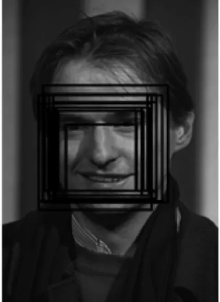
Similar to the pyramid image to shrink an image, the shrink factor is set to K = 1:1, as shown in Figure 11. Here, we use the resized function of Open CV to shrink the image. Parameter CV INTER AREA can be used to nd moire' free results. Generally, a larger shrink factor, K, can further shrink the image with a higher detection speed, but part of the face may not be detected. The sub-window moves two pixels in each direction. The smaller moved distance may increase computation time with more precision; the larger moved distance may reduce computation time but possibly skip the face. In the face detection pro-cessing, it may repeatedly produce overlapped frames, as shown in Figure 12. Each frame represents that the face has been detected once, and there are several dierent detection positions on the same face, due to the dierent face sizes and positions of the training samples. According to the relative position of the overlapping blocks in the process, it can determine whether it is the same face or not, as shown in Figure 13, where C < A=2 and D < B=2.
4. Experimental results and analysis
We trained three architectures and compared them with each other:
Figure 12. Repeatedly detecting the human face block.
Figure 13. Overlapped block diagram.
1. Using the proposed face detection cascade architec-ture to train MCT and GBP;
2. Using the Adaboost algorithm [1,2] to train the rectangular features;
3. Using the BGSLDA algorithm [6] to train the rectangular features.
4.1. Samples training
In this study, the face samples used include:
1. MIT CMU [21] face database with a total of 2,429 faces;
2. BioID [22] face database with a total of 1,521 faces;
3. CALTECH face database [23] with a total of 60 faces.
Table 2. Algorithms and features trained in this study. Method Feature Number of trained data
Adaboost [1,2] MCT 483
Haar-like 59
BGSLDA [6] Haar-like 58
BPN GBP 576
The total faces are 4,010. The face samples from databases 2) and 3) are obtained by extraction, and the positions are mostly between the eyebrows and mouth. The non-face sample set does not contain face images, with a total of 4,010 images. Considering operation and performance, all samples were scaled to the sub-window size of 24 24. Before training the GBP, we used HE to process the samples. This study completely trained the three algorithms and three features, as shown in Table 2. The MCT trained a total of 483 points. In Adaboost (Haar-like), the rectangular features, in-cluding features of upright and 45 [24], were trained
with 10 stages and 59 features. In BGSLDA (Haar-like), the rectangular features, including features of upright and 45 [24], were trained with 6 stages and 58
features. BPN collocated with GBP to train a total of 576 features. For BPN, one input layer has 576 nodes; one hidden layer has 80 nodes, and one output layer has one node. If the output value approximates 1, it is classied as a face. On the other hand, if the output value approximates 0, it is classied as a non-face (The threshold value is set to the middle value, 0.5). The minimum acceptable DR of Adaboost (Haar-like) and BGSLDA (Haar-like) is set to 99.5%, and the maximum acceptable FPR is set to 50%. If the window of MCT is greater than or equal to 5 5, the data quantity becomes too huge (greater than 40 GB). Therefore, the window size of MCT is set to 3 3 in this work. 4.2. Performance comparisons and analysis In order to verify the proposed face detection architec-ture, we use three test databases:
1. AT&T face database [25] with a total of 400 faces;
2. Gray FERET face database [26] that uses fa, fb, ba, bj, and bk images with a total of 3,133 faces;
3. 100 single face images with 320 240 resolution. The performance comparisons are shown in Table 3. Eq. (10) is used to calculate the DR.
DR = Detected facesTotal faces 100%: (10) The proposed architecture performed DR of 99% and false positives of 11. For Adaboost with rectangular features [1,2], DR is 99.15% and false positives of 131,048. For BGSLDA with rectangular features [6], DR is 99.83% and false positives of 194,907. To-tal scanned sub-windows are 337,915,906 in the test databases [25,26].
The single face image with a resolution of 320 240 is used to evaluate the detection speed. The proposed architecture performs a detection speed of 27.92 FPS, which can achieve the goal of real-time detection, as shown in Table 3. In [1,2], the detection speed is 26.89 FPS, and in [6], the detection speed is 25.55 FPS. The experiment shows that based on detec-tion performance and speed, the proposed architecture outperforms that of [1,2,6].
In addition, we also compare the detection per-formance at dierent illuminations. The MUCT [27] color frontal face database is used to extract part of the face; the extracted image is then shrunk to a resolution of 24 24 pixels, and, nally, transformed to the grayscale image, as shown in Figure 14. It has a total of 751 images, which contain 77 dark images, 475 normal illumination images, and 199 bright images for positive test samples. The negative test samples contain 20,736 images without a face. Then, we compared the three architectures of the Receiver Operating Characteristic (ROC) curve in Figure 15. It
Figure 14. The part of positive test samples for the ROC comparison.
Table 3. The performance comparison.
Methods Correct detections DR False detections Computing time Adaboost (Haar-like) [1,2] 3,503 99.15% 131,048 26.89 FPS
BGSLDA (Haar-like) [6] 3,527 99.83% 194,907 25.55 FPS
Figure 15. The ROC curves for comparisons.
shows that the proposed face detection architecture has a very good performance under various illuminations. 5. Conclusion
In this paper, we proposed a new face detection architecture to combine Adaboost and BPN algorithms for an illumination variant environment. The Adaboost algorithm collocated with MCT not only reduces the impact of illumination, but also saves the preprocessing time. It uses the concept of hierarchical features to control the number of features to limit the operation time for each sub-window. BPN collocated with GBP can compensate for the brightness information removed by MCT. This architecture can take into account the accuracy and immediate response. The overall architecture has DR of 99%, FPR of 11, and a detection speed of 27.92 FPS. The experimental results show that with the same samples, the accuracy and detection speed of the proposed system are better than those of the Adaboost and BGSLDA cascade architecture collocated with rectangular features.
References
1. Viola, P. and Jones, M. \Rapid object detection
using a boosted cascade of simple features", Computer Vision and Pattern Recognition, 1, pp. 511-518 (2001).
2. Viola, P. and Jones, M. \Robust real-time face
de-tection", International Journal of Computer Vision, 57(2), pp. 137-154 (2004).
3. Ali, K., Fleuret, F., Hasler, D. and Fua, P. \A real-time
deformable detector", IEEE Transactions on Pattern Analysis and Machine Intelligence, 34(2), pp. 225-239 (2012).
4. Masnadi-Shirazi, H. and Vasconcelos, N.
\Cost-sensitive boosting", IEEE Transactions on Pattern Analysis and Machine Intelligence, 33(2), pp. 294-309 (2011).
5. Wang, P., Shen, C., Barnes, N. and Zheng, H. \Fast
and robust object detection using asymmetric totally corrective boosting", IEEE Transactions on Neural
Networks and Learning Systems, 23(1), pp. 33-46 (2012).
6. Shen, C., Paisitkriangkrai, S. and Zhang, J.
\E-ciently learning a detection cascade with sparse eigen-vectors", IEEE Transactions on Image Processing, 20(1), pp. 22-35 (2011).
7. Shi, P. and Liu, C. \Face detection using
discrimi-nating feature analysis and support vector machine", Pattern Recognition, 39(2), pp. 260-276 (2006).
8. Guo, J.-M., Lin, C.-C., Wu, M.-F., Chang, C.-H.
and Lee, H. \Complexity reduced face detection using probability-based face mask preltering and pixel-based hierarchical-feature Adaboosting", IEEE Signal Processing Letters, 18(8), pp. 447-450 (2011).
9. Ghimire, D. and Lee, J. \A lighting insensitive face
detection method on color images", Spring Congress on Engineering and Technology, Xi'an, China, pp. 1-4 (2012).
10. Liu, Q. and Peng, G.-Z. \A robust skin color based face
detection algorithm", International Asia Conference on Informatics in Control, Automation and Robotics, 2, Wuhan, China, pp. 525-528 (2010).
11. Powar, V. and Jahagirdar, A. \Reliable face detection
in varying illumination and complex background", In-ternational Conference on Communication, Informa-tion & Computing Technology, Munshi Nagar Mumbai, India, pp. 1-4 (2012).
12. Wang, Y.-H. and Xia, L.-Q. \Skin color and
feature-based face detection in complicated backgrounds", In-ternational Conference on Image Analysis and Signal Processing, Hubei, China, pp. 78-83 (2011).
13. Ng, P. and Pun, C.-M. \Skin segmentation based on
human face illumination feature", IEEE/WIC/ACM International Joint Conference on Web Intelligence and Intelligent Agent Technology, Macau, China, pp. 373-377 (2012).
14. Tan, W.-R., Chan, C.-S., Yogarajah, P. and Condell, J.
\A fusion approach for ecient human skin detection", IEEE Transactions on Industrial Informatics, 8(1), pp. 138-147 (2012).
15. Liu, L., Sang, N., Yang, S. and Huang, R. \Real-time
skin color detection under rapidly changing illumi-nation conditions", IEEE Transactions on Consumer Electronics, 57(3), pp. 1295-1302 (2011).
16. Herout, A., Josth, R., Juranek, R., Havel, J., Hradis,
M. and Zemck, P. \Real-time object detection on CUDA", Journal of Real-Time Image Processing, 6, pp. 159-170 (2011).
17. Lau, B.T. \Portable real time emotion detection
sys-tem for the disabled", Expert Syssys-tems with Applica-tions, 37(9), pp. 6561-6566 (2010).
18. Danisman, T., Bilasco, I.M., Martinet, J. and Djeraba,
C. \Intelligent pixels of interest selection with applica-tion to facial expression recogniapplica-tion using multilayer perceptron", Signal Processing, 93(6), pp. 1547-1556 (2013).
19. Froba, B. and Ernst, A. \Face detection with the modi-ed census transform", IEEE International Conference on Automatic Face and Gesture Recognition, Seoul, Korea, pp. 91-96 (2004).
20. Zabih, R. and Woodll, J. \A non-parametric
ap-proach to visual correspondence", IEEE Transactions on Pattern Analysis and Machine Intelligence (1996).
21. MIT CMU face database [Online]. Available: http://
cbcl.mit.edu/cbcl/software-datasets/FaceData2.html
22. BioIDface database [Online]. Available: http://www.
bioid.com/downloads/software/bioid-face-database. html
23. CALTECH face database [Online]. Available: http://
www.vision.caltech.edu/html-les/archive.html
24. Lienhart, R. and Maydt, J. \An extended set of
Haar-like features for rapid object detection", IEEE International Conference on Image Processing, 1, pp. 900-903 (September, 2002).
25. AT&T face database [Online]. Available: http://www.
cl.cam.ac.uk/research/dtg/attarchive/facedatabase. html
26. FERET face database [Online]. Available:
http://ww-w.itl.nist.gov/iad/humanid/feret/feret master.html
27. MUCT face database [Online], Available: http://www.
milbo.org/muct/
Biographies
Chih-Hsien Hsia was born in Taipei city, Taiwan, in 1979. He received a BS degree in Computer Science and Information Engineering from Taipei Chengshih University of Science and Technology, Taipei, Taiwan, in 2003, and MS and PhD degrees in Electrical Engi-neering from Tamkang University, New Taipei, Taiwan, in 2005 and 2010, respectively.
He was a Visiting Scholar with Iowa State
Uni-versity, Ames, USA, in 2007, and from 2010 to 2013, he was a Post-Doctoral Research Fellow with the Department of Electrical Engineering at the National Taiwan University of Science and Technology, Taipei, Taiwan. He is currently Associate Professor in the Department of Electrical Engineering at the Chinese Cultural University, Taipei, Taiwan. His research interests include DSP IC design, image/video com-pression system, multimedia signal processing, and computer/robot vision processing.
Dr. Hsia is a member of the IEEE, and Phi Tau Phi scholastic honor society. He has served as Guest Editor for special issues of the Journal of Applied Science and Engineering.
Jen-Shiun Chiang received a BS degree in Elec-tronics Engineering from Tamkang University, Taipei, Taiwan, in 1983, an MS degree in Electrical Engi-neering from the University of Idaho, USA, in 1988, and a PhD degree in electrical engineering from Texas A&M University, Texas, USA, in 1992. Currently he is Professor in the Department of Electrical Engineering at Tamkang University. His research interests include digital signal processing for VLSI architecture, archi-tecture for image data compressing, SoC design, analog to digital data conversion, and low power circuit design. Prof. Chiang is a member of IEEE, and a Fellow of IET. He has served as Associate Editor of Integration, and the VLSI Journal, and is on the Editorial Board of the Journal of Applied Science and Engineering. Chin-Yi Lin received a BS degree in Electrical Engi-neering from Chung-Hua University, Taipei, Taiwan, in 2008, and an MS degree in Electrical Engineering from Tamkang University, New Taipei, Taiwan, in 2011.
His research interests include digital IC design and computer vision processing.