IBM SPSS Statistics Base 22
Note
Before using this information and the product it supports, read the information in “Notices” on page 179.
Contents
Chapter 1. Codebook . . . 1
Codebook Output Tab . . . 1
Codebook Statistics Tab. . . 3
Chapter 2. Frequencies . . . 5
Frequencies Statistics . . . 5
Frequencies Charts . . . 7
Frequencies Format . . . 7
Chapter 3. Descriptives . . . 9
Descriptives Options. . . 9
DESCRIPTIVES Command Additional Features . . 10
Chapter 4. Explore . . . 11
Explore Statistics . . . 12
Explore Plots . . . 12
Explore Power Transformations. . . 12
Explore Options . . . 13
EXAMINE Command Additional Features . . . . 13
Chapter 5. Crosstabs
. . . 15
Crosstabs layers . . . 16
Crosstabs clustered bar charts . . . 16
Crosstabs displaying layer variables in table layers 16 Crosstabs statistics . . . 16
Crosstabs cell display . . . 18
Crosstabs table format . . . 19
Chapter 6. Summarize . . . 21
Summarize Options . . . 21
Summarize Statistics . . . 22
Chapter 7. Means . . . 25
Means Options . . . 25
Chapter 8. OLAP Cubes . . . 29
OLAP Cubes Statistics . . . 29
OLAP Cubes Differences . . . 31
OLAP Cubes Title . . . 31
Chapter 9. T Tests . . . 33
T Tests . . . 33
Independent-Samples T Test . . . 33
Independent-Samples T Test Define Groups . . 34
Independent-Samples T Test Options . . . 34
Paired-Samples T Test . . . 34
Paired-Samples T Test Options . . . 35
T-TEST Command Additional Features . . . . 35
One-Sample T Test . . . 35
One-Sample T Test Options . . . 36
T-TEST Command Additional Features . . . . 36
T-TEST Command Additional Features . . . 36
Chapter 10. One-Way ANOVA . . . 37
One-Way ANOVA Contrasts . . . 37
One-Way ANOVA Post Hoc Tests . . . 38
One-Way ANOVA Options . . . 39
ONEWAY Command Additional Features . . . . 40
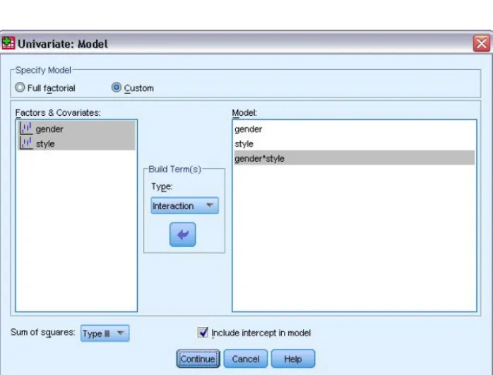
Chapter 11. GLM Univariate Analysis
41
GLM Model . . . 42Build Terms . . . 43
Sum of Squares . . . 43
GLM Contrasts . . . 44
Contrast Types . . . 44
GLM Profile Plots . . . 44
GLM Options. . . 45
UNIANOVA Command Additional Features . . 45
GLM Post Hoc Comparisons . . . 46
GLM Options. . . 47
UNIANOVA Command Additional Features . . 48
GLM Save . . . 48
GLM Options. . . 49
UNIANOVA Command Additional Features . . . 50
Chapter 12. Bivariate Correlations . . . 51
Bivariate Correlations Options . . . 51
CORRELATIONS and NONPAR CORR Command Additional Features. . . 52
Chapter 13. Partial Correlations . . . . 53
Partial Correlations Options . . . 53
PARTIAL CORR Command Additional Features . . 54
Chapter 14. Distances . . . 55
Distances Dissimilarity Measures . . . 55
Distances Similarity Measures . . . 56
PROXIMITIES Command Additional Features . . . 56
Chapter 15. Linear models . . . 57
To obtain a linear model . . . 57
Objectives . . . 57
Basics . . . 58
Model Selection . . . 58
Ensembles . . . 59
Advanced . . . 59
Model Options . . . 60
Model Summary. . . 60
Automatic Data Preparation . . . 60
Predictor Importance . . . 61
Predicted By Observed . . . 61
Residuals . . . 61
Outliers . . . 61
Effects . . . 61
Coefficients . . . 62
Estimated Means . . . 62
Chapter 16. Linear Regression
. . . . 65
Linear Regression Variable Selection Methods . . . 66
Linear Regression Set Rule . . . 66
Linear Regression Plots . . . 66
Linear Regression: Saving New Variables . . . . 67
Linear Regression Statistics . . . 68
Linear Regression Options . . . 69
REGRESSION Command Additional Features . . . 70
Chapter 17. Ordinal Regression . . . . 71
Ordinal Regression Options . . . 72
Ordinal Regression Output . . . 72
Ordinal Regression Location Model . . . 73
Build Terms . . . 73
Ordinal Regression Scale Model . . . 73
Build Terms . . . 73
PLUM Command Additional Features . . . 74
Chapter 18. Curve Estimation . . . 75
Curve Estimation Models. . . 76
Curve Estimation Save . . . 76
Chapter 19. Partial Least Squares
Regression . . . 79
Model . . . 80
Options. . . 81
Chapter 20. Nearest Neighbor Analysis
83
Neighbors . . . 85Features . . . 85
Partitions . . . 86
Save . . . 87
Output . . . 87
Options. . . 87
Model View . . . 88
Feature Space. . . 88
Variable Importance . . . 89
Peers . . . 89
Nearest Neighbor Distances . . . 90
Quadrant map . . . 90
Feature selection error log . . . 90
k selection error log . . . 90
k and Feature Selection Error Log . . . 90
Classification Table . . . 90
Error Summary . . . 90
Chapter 21. Discriminant Analysis . . . 91
Discriminant Analysis Define Range . . . 92
Discriminant Analysis Select Cases . . . 92
Discriminant Analysis Statistics . . . 92
Discriminant Analysis Stepwise Method . . . 93
Discriminant Analysis Classification . . . 93
Discriminant Analysis Save . . . 94
DISCRIMINANT Command Additional Features . . 94
Chapter 22. Factor Analysis. . . 95
Factor Analysis Select Cases . . . 96
Factor Analysis Descriptives . . . 96
Factor Analysis Extraction . . . 96
Factor Analysis Rotation . . . 97
Factor Analysis Scores . . . 98
Factor Analysis Options . . . 98
FACTOR Command Additional Features . . . . 98
Chapter 23. Choosing a Procedure for
Clustering . . . 99
Chapter 24. TwoStep Cluster Analysis
101
TwoStep Cluster Analysis Options . . . 102TwoStep Cluster Analysis Output . . . 103
The Cluster Viewer . . . 104
Cluster Viewer . . . 104
Navigating the Cluster Viewer . . . 107
Filtering Records . . . 108
Chapter 25. Hierarchical Cluster
Analysis
. . . 109
Hierarchical Cluster Analysis Method . . . 109
Hierarchical Cluster Analysis Statistics . . . 110
Hierarchical Cluster Analysis Plots . . . 110
Hierarchical Cluster Analysis Save New Variables 110 CLUSTER Command Syntax Additional Features 110
Chapter 26. K-Means Cluster Analysis
111
K-Means Cluster Analysis Efficiency . . . 112K-Means Cluster Analysis Iterate . . . 112
K-Means Cluster Analysis Save . . . 112
K-Means Cluster Analysis Options . . . 112
QUICK CLUSTER Command Additional Features 113
Chapter 27. Nonparametric Tests . . . 115
One-Sample Nonparametric Tests. . . 115
To Obtain One-Sample Nonparametric Tests . . 115
Fields Tab . . . 115
Settings Tab . . . 116
NPTESTS Command Additional Features . . . 118
Independent-Samples Nonparametric Tests . . . 118
To Obtain Independent-Samples Nonparametric Tests . . . 118
Fields Tab . . . 118
Settings Tab . . . 119
NPTESTS Command Additional Features . . . 120
Related-Samples Nonparametric Tests . . . 120
To Obtain Related-Samples Nonparametric Tests 121 Fields Tab . . . 121
Settings Tab . . . 121
NPTESTS Command Additional Features . . . 123
Model View . . . 123
Model View . . . 123
NPTESTS Command Additional Features . . . . 127
Legacy Dialogs . . . 127
Chi-Square Test. . . 128
Binomial Test . . . 129
Runs Test. . . 130
One-Sample Kolmogorov-Smirnov Test . . . . 131
Two-Independent-Samples Tests . . . 132
Two-Related-Samples Tests . . . 134
Tests for Several Related Samples. . . 136
Chapter 28. Multiple Response
Analysis
. . . 139
Multiple Response Analysis . . . 139
Multiple Response Define Sets. . . 139
Multiple Response Frequencies . . . 140
Multiple Response Crosstabs . . . 141
Multiple Response Crosstabs Define Ranges . . 142
Multiple Response Crosstabs Options . . . . 142
MULT RESPONSE Command Additional Features . . . 142
Chapter 29. Reporting Results . . . . 143
Reporting Results . . . 143
Report Summaries in Rows. . . 143
To Obtain a Summary Report: Summaries in Rows . . . 143
Report Data Column/Break Format . . . 144
Report Summary Lines for/Final Summary Lines . . . 144
Report Break Options . . . 144
Report Options . . . 144
Report Layout . . . 145
Report Titles. . . 145
Report Summaries in Columns . . . 145
To Obtain a Summary Report: Summaries in Columns . . . 146
Data Columns Summary Function . . . 146
Data Columns Summary for Total Column . . 146
Report Column Format . . . 147
Report Summaries in Columns Break Options 147 Report Summaries in Columns Options . . . 147
Report Layout for Summaries in Columns. . . 147
REPORT Command Additional Features . . . . 147
Chapter 30. Reliability Analysis. . . . 149
Reliability Analysis Statistics . . . 149
RELIABILITY Command Additional Features. . . 151
Chapter 31. Multidimensional Scaling
153
Multidimensional Scaling Shape of Data . . . . 154Multidimensional Scaling Create Measure . . . . 154
Multidimensional Scaling Model . . . 154
Multidimensional Scaling Options . . . 155
ALSCAL Command Additional Features . . . . 155
Chapter 32. Ratio Statistics . . . 157
Ratio Statistics . . . 157
Chapter 33. ROC Curves
. . . 159
ROC Curve Options . . . 159
Chapter 34. Simulation . . . 161
To design a simulation based on a model file . . . 161
To design a simulation based on custom equations 162 To design a simulation without a predictive model 162 To run a simulation from a simulation plan . . . 163
Simulation Builder . . . 164
Model tab . . . 164
Simulation tab . . . 166
Run Simulation dialog . . . 174
Simulation tab . . . 174
Output tab . . . 175
Working with chart output from Simulation . . . 177
Chart Options . . . 177
Notices . . . 179
Trademarks . . . 181
Chapter 1. Codebook
Codebook reports the dictionary information -- such as variable names, variable labels, value labels, missing values -- and summary statistics for all or specified variables and multiple response sets in the active dataset. For nominal and ordinal variables and multiple response sets, summary statistics include counts and percents. For scale variables, summary statistics include mean, standard deviation, and quartiles.
Note: Codebook ignores split file status. This includes split-file groups created for multiple imputation of missing values (available in the Missing Values add-on option).
To Obtain a Codebook 1. From the menus choose:
Analyze>Reports>Codebook 2. Click the Variables tab.
3. Select one or more variables and/or multiple response sets. Optionally, you can:
v Control the variable information that is displayed.
v Control the statistics that are displayed (or exclude all summary statistics). v Control the order in which variables and multiple response sets are displayed.
v Change the measurement level for any variable in the source list in order to change the summary statistics displayed. See the topic “Codebook Statistics Tab” on page 3 for more information. Changing Measurement Level
You can temporarily change the measurement level for variables. (You cannot change the measurement level for multiple response sets. They are always treated as nominal.)
1. Right-click a variable in the source list.
2. Select a measurement level from the pop-up menu.
This changes the measurement level temporarily. In practical terms, this is only useful for numeric variables. The measurement level for string variables is restricted to nominal or ordinal, which are both treated the same by the Codebook procedure.
Codebook Output Tab
The Output tab controls the variable information included for each variable and multiple response set, the order in which the variables and multiple response sets are displayed, and the contents of the optional file information table.
Variable Information
This controls the dictionary information displayed for each variable.
Position.An integer that represents the position of the variable in file order. This is not available for multiple response sets.
Type.Fundamental data type. This is eitherNumeric,String, orMultiple Response Set.
Format.The display format for the variable, such asA4,F8.2, orDATE11. This is not available for multiple response sets.
Measurement level.The possible values areNominal,Ordinal,Scale, andUnknown. The value displayed is the measurement level stored in the dictionary and is not affected by any temporary measurement level override specified by changing the measurement level in the source variable list on the Variables tab. This is not available for multiple response sets.
Note: The measurement level for numeric variables may be "unknown" prior to the first data pass when the measurement level has not been explicitly set, such as data read from an external source or newly created variables. See the topic for more information.
Role.Some dialogs support the ability to pre-select variables for analysis based on defined roles. Value labels.Descriptive labels associated with specific data values.
v If Count or Percent is selected on the Statistics tab, defined value labels are included in the output even if you don't select Value labels here.
v For multiple dichotomy sets, "value labels" are either the variable labels for the elementary variables in the set or the labels of counted values, depending on how the set is defined. See the topic for more information.
Missing values.User-defined missing values. If Count or Percent is selected on the Statistics tab, defined value labels are included in the output even if you don't select Missing values here. This is not available for multiple response sets.
Custom attributes.User-defined custom variable attributes. Output includes both the names and values for any custom variable attributes associated with each variable. See the topic for more information. This is not available for multiple response sets.
Reserved attributes.Reserved system variable attributes. You can display system attributes, but you should not alter them. System attribute names start with a dollar sign ($) . Non-display attributes, with names that begin with either "@" or "$@", are not included. Output includes both the names and values for any system attributes associated with each variable. This is not available for multiple response sets. File Information
The optional file information table can include any of the following file attributes:
File name.Name of the IBM®SPSS®Statistics data file. If the dataset has never been saved in IBM SPSS
Statistics format, then there is no data file name. (If there is no file name displayed in the title bar of the Data Editor window, then the active dataset does not have a file name.)
Location.Directory (folder) location of the IBM SPSS Statistics data file. If the dataset has never been saved in IBM SPSS Statistics format, then there is no location.
Number of cases.Number of cases in the active dataset. This is the total number of cases, including any cases that may be excluded from summary statistics due to filter conditions.
Label.This is the file label (if any) defined by theFILE LABELcommand. Documents.Data file document text.
Weight status.If weighting is on, the name of the weight variable is displayed. See the topic for more information.
Custom attributes.User-defined custom data file attributes. Data file attributes defined with theDATAFILE ATTRIBUTEcommand.
Reserved attributes.Reserved system data file attributes. You can display system attributes, but you should not alter them. System attribute names start with a dollar sign ($) . Non-display attributes, with names that begin with either "@" or "$@", are not included. Output includes both the names and values for any system data file attributes.
Variable Display Order
The following alternatives are available for controlling the order in which variables and multiple response sets are displayed.
Alphabetical.Alphabetic order by variable name.
File.The order in which variables appear in the dataset (the order in which they are displayed in the Data Editor). In ascending order, multiple response sets are displayed last, after all selected variables. Measurement level.Sort by measurement level. This creates four sorting groups: nominal, ordinal, scale, and unknown. Multiple response sets are treated as nominal.
Note: The measurement level for numeric variables may be "unknown" prior to the first data pass when the measurement level has not been explicitly set, such as data read from an external source or newly created variables.
Variable list.The order in which variables and multiple response sets appear in the selected variables list on the Variables tab.
Custom attribute name.The list of sort order options also includes the names of any user-defined custom variable attributes. In ascending order, variables that don't have the attribute sort to the top, followed by variables that have the attribute but no defined value for the attribute, followed by variables with defined values for the attribute in alphabetic order of the values.
Maximum Number of Categories
If the output includes value labels, counts, or percents for each unique value, you can suppress this information from the table if the number of values exceeds the specified value. By default, this information is suppressed if the number of unique values for the variable exceeds 200.
Codebook Statistics Tab
The Statistics tab allows you to control the summary statistics that are included in the output, or suppress the display of summary statistics entirely.
Counts and Percents
For nominal and ordinal variables, multiple response sets, and labeled values of scale variables, the available statistics are:
Count. The count or number of cases having each value (or range of values) of a variable.
Central Tendency and Dispersion
For scale variables, the available statistics are:
Mean. A measure of central tendency. The arithmetic average, the sum divided by the number of cases.
Standard Deviation. A measure of dispersion around the mean. In a normal distribution, 68% of cases fall within one standard deviation of the mean and 95% of cases fall within two standard deviations. For example, if the mean age is 45, with a standard deviation of 10, 95% of the cases would be between 25 and 65 in a normal distribution.
Quartiles. Displays values corresponding to the 25th, 50th, and 75th percentiles.
Note: You can temporarily change the measurement level associated with a variable (and thereby change the summary statistics displayed for that variable) in the source variable list on the Variables tab.
Chapter 2. Frequencies
The Frequencies procedure provides statistics and graphical displays that are useful for describing many types of variables. The Frequencies procedure is a good place to start looking at your data.
For a frequency report and bar chart, you can arrange the distinct values in ascending or descending order, or you can order the categories by their frequencies. The frequencies report can be suppressed when a variable has many distinct values. You can label charts with frequencies (the default) or percentages.
Example.What is the distribution of a company's customers by industry type? From the output, you might learn that 37.5% of your customers are in government agencies, 24.9% are in corporations, 28.1% are in academic institutions, and 9.4% are in the healthcare industry. For continuous, quantitative data, such as sales revenue, you might learn that the average product sale is $3,576, with a standard deviation of $1,078.
Statistics and plots.Frequency counts, percentages, cumulative percentages, mean, median, mode, sum, standard deviation, variance, range, minimum and maximum values, standard error of the mean, skewness and kurtosis (both with standard errors), quartiles, user-specified percentiles, bar charts, pie charts, and histograms.
Frequencies Data Considerations
Data.Use numeric codes or strings to code categorical variables (nominal or ordinal level measurements). Assumptions.The tabulations and percentages provide a useful description for data from any
distribution, especially for variables with ordered or unordered categories. Most of the optional summary statistics, such as the mean and standard deviation, are based on normal theory and are appropriate for quantitative variables with symmetric distributions. Robust statistics, such as the median, quartiles, and percentiles, are appropriate for quantitative variables that may or may not meet the assumption of normality.
To Obtain Frequency Tables 1. From the menus choose:
Analyze>Descriptive Statistics> Frequencies... 2. Select one or more categorical or quantitative variables. Optionally, you can:
v ClickStatistics for descriptive statistics for quantitative variables. v ClickChartsfor bar charts, pie charts, and histograms.
v ClickFormatfor the order in which results are displayed.
Frequencies Statistics
Percentile Values.Values of a quantitative variable that divide the ordered data into groups so that a certain percentage is above and another percentage is below. Quartiles (the 25th, 50th, and 75th percentiles) divide the observations into four groups of equal size. If you want an equal number of groups other than four, selectCut points for n equal groups.You can also specify individual percentiles (for example, the 95th percentile, the value below which 95% of the observations fall).
Central Tendency.Statistics that describe the location of the distribution include the mean, median, mode, and sum of all the values.
v Mean. A measure of central tendency. The arithmetic average, the sum divided by the number of cases. v Median. The value above and below which half of the cases fall, the 50th percentile. If there is an even
number of cases, the median is the average of the two middle cases when they are sorted in ascending or descending order. The median is a measure of central tendency not sensitive to outlying values (unlike the mean, which can be affected by a few extremely high or low values).
v Mode. The most frequently occurring value. If several values share the greatest frequency of occurrence, each of them is a mode. The Frequencies procedure reports only the smallest of such multiple modes.
v Sum. The sum or total of the values, across all cases with nonmissing values.
Dispersion.Statistics that measure the amount of variation or spread in the data include the standard deviation, variance, range, minimum, maximum, and standard error of the mean.
v Std. deviation. A measure of dispersion around the mean. In a normal distribution, 68% of cases fall within one standard deviation of the mean and 95% of cases fall within two standard deviations. For example, if the mean age is 45, with a standard deviation of 10, 95% of the cases would be between 25 and 65 in a normal distribution.
v Variance. A measure of dispersion around the mean, equal to the sum of squared deviations from the mean divided by one less than the number of cases. The variance is measured in units that are the square of those of the variable itself.
v Range. The difference between the largest and smallest values of a numeric variable, the maximum minus the minimum.
v Minimum. The smallest value of a numeric variable. v Maximum. The largest value of a numeric variable.
v S. E. mean. A measure of how much the value of the mean may vary from sample to sample taken from the same distribution. It can be used to roughly compare the observed mean to a hypothesized value (that is, you can conclude the two values are different if the ratio of the difference to the standard error is less than -2 or greater than +2).
Distribution.Skewness and kurtosis are statistics that describe the shape and symmetry of the distribution. These statistics are displayed with their standard errors.
v Skewness. A measure of the asymmetry of a distribution. The normal distribution is symmetric and has a skewness value of 0. A distribution with a significant positive skewness has a long right tail. A distribution with a significant negative skewness has a long left tail. As a guideline, a skewness value more than twice its standard error is taken to indicate a departure from symmetry.
v Kurtosis. A measure of the extent to which observations cluster around a central point. For a normal distribution, the value of the kurtosis statistic is zero. Positive kurtosis indicates that, relative to a normal distribution, the observations are more clustered about the center of the distribution and have thinner tails until the extreme values of the distribution, at which point the tails of the leptokurtic distribution are thicker relative to a normal distribution. Negative kurtosis indicates that, relative to a normal distribution, the observations cluster less and have thicker tails until the extreme values of the distribution, at which point the tails of the platykurtic distribution are thinner relative to a normal distribution.
Values are group midpoints.If the values in your data are midpoints of groups (for example, ages of all people in their thirties are coded as 35), select this option to estimate the median and percentiles for the original, ungrouped data.
Frequencies Charts
Chart Type.A pie chart displays the contribution of parts to a whole. Each slice of a pie chart
corresponds to a group that is defined by a single grouping variable. A bar chart displays the count for each distinct value or category as a separate bar, allowing you to compare categories visually. A
histogram also has bars, but they are plotted along an equal interval scale. The height of each bar is the count of values of a quantitative variable falling within the interval. A histogram shows the shape, center, and spread of the distribution. A normal curve superimposed on a histogram helps you judge whether the data are normally distributed.
Chart Values.For bar charts, the scale axis can be labeled by frequency counts or percentages.
Frequencies Format
Order by.The frequency table can be arranged according to the actual values in the data or according to the count (frequency of occurrence) of those values, and the table can be arranged in either ascending or descending order. However, if you request a histogram or percentiles, Frequencies assumes that the variable is quantitative and displays its values in ascending order.
Multiple Variables.If you produce statistics tables for multiple variables, you can either display all variables in a single table (Compare variables) or display a separate statistics table for each variable (Organize output by variables).
Suppress tables with many categories.This option prevents the display of tables with more than the specified number of values.
Chapter 3. Descriptives
The Descriptives procedure displays univariate summary statistics for several variables in a single table and calculates standardized values (zscores). Variables can be ordered by the size of their means (in ascending or descending order), alphabetically, or by the order in which you select the variables (the default).
Whenzscores are saved, they are added to the data in the Data Editor and are available for charts, data listings, and analyses. When variables are recorded in different units (for example, gross domestic product per capita and percentage literate), az-score transformation places variables on a common scale for easier visual comparison.
Example.If each case in your data contains the daily sales totals for each member of the sales staff (for example, one entry for Bob, one entry for Kim, and one entry for Brian) collected each day for several months, the Descriptives procedure can compute the average daily sales for each staff member and can order the results from highest average sales to lowest average sales.
Statistics.Sample size, mean, minimum, maximum, standard deviation, variance, range, sum, standard error of the mean, and kurtosis and skewness with their standard errors.
Descriptives Data Considerations
Data.Use numeric variables after you have screened them graphically for recording errors, outliers, and distributional anomalies. The Descriptives procedure is very efficient for large files (thousands of cases). Assumptions.Most of the available statistics (includingzscores) are based on normal theory and are appropriate for quantitative variables (interval- or ratio-level measurements) with symmetric
distributions. Avoid variables with unordered categories or skewed distributions. The distribution ofz
scores has the same shape as that of the original data; therefore, calculatingzscores is not a remedy for problem data.
To Obtain Descriptive Statistics 1. From the menus choose:
Analyze>Descriptive Statistics> Descriptives... 2. Select one or more variables.
Optionally, you can:
v SelectSave standardized values as variablesto savezscores as new variables. v ClickOptionsfor optional statistics and display order.
Descriptives Options
Mean and Sum.The mean, or arithmetic average, is displayed by default.
Dispersion.Statistics that measure the spread or variation in the data include the standard deviation, variance, range, minimum, maximum, and standard error of the mean.
v Std. deviation. A measure of dispersion around the mean. In a normal distribution, 68% of cases fall within one standard deviation of the mean and 95% of cases fall within two standard deviations. For example, if the mean age is 45, with a standard deviation of 10, 95% of the cases would be between 25 and 65 in a normal distribution.
v Variance. A measure of dispersion around the mean, equal to the sum of squared deviations from the mean divided by one less than the number of cases. The variance is measured in units that are the square of those of the variable itself.
v Range. The difference between the largest and smallest values of a numeric variable, the maximum minus the minimum.
v Minimum. The smallest value of a numeric variable. v Maximum. The largest value of a numeric variable.
v S.E. mean. A measure of how much the value of the mean may vary from sample to sample taken from the same distribution. It can be used to roughly compare the observed mean to a hypothesized value (that is, you can conclude the two values are different if the ratio of the difference to the standard error is less than -2 or greater than +2).
Distribution.Kurtosis and skewness are statistics that characterize the shape and symmetry of the distribution. These statistics are displayed with their standard errors.
v Kurtosis. A measure of the extent to which observations cluster around a central point. For a normal distribution, the value of the kurtosis statistic is zero. Positive kurtosis indicates that, relative to a normal distribution, the observations are more clustered about the center of the distribution and have thinner tails until the extreme values of the distribution, at which point the tails of the leptokurtic distribution are thicker relative to a normal distribution. Negative kurtosis indicates that, relative to a normal distribution, the observations cluster less and have thicker tails until the extreme values of the distribution, at which point the tails of the platykurtic distribution are thinner relative to a normal distribution.
v Skewness. A measure of the asymmetry of a distribution. The normal distribution is symmetric and has a skewness value of 0. A distribution with a significant positive skewness has a long right tail. A distribution with a significant negative skewness has a long left tail. As a guideline, a skewness value more than twice its standard error is taken to indicate a departure from symmetry.
Display Order.By default, the variables are displayed in the order in which you selected them. Optionally, you can display variables alphabetically, by ascending means, or by descending means.
DESCRIPTIVES Command Additional Features
The command syntax language also allows you to:
v Save standardized scores (zscores) for some but not all variables (with theVARIABLESsubcommand). v Specify names for new variables that contain standardized scores (with theVARIABLESsubcommand). v Exclude from the analysis cases with missing values for any variable (with theMISSING subcommand). v Sort the variables in the display by the value of any statistic, not just the mean (with theSORT
subcommand).
Chapter 4. Explore
The Explore procedure produces summary statistics and graphical displays, either for all of your cases or separately for groups of cases. There are many reasons for using the Explore procedure--data screening, outlier identification, description, assumption checking, and characterizing differences among
subpopulations (groups of cases). Data screening may show that you have unusual values, extreme values, gaps in the data, or other peculiarities. Exploring the data can help to determine whether the statistical techniques that you are considering for data analysis are appropriate. The exploration may indicate that you need to transform the data if the technique requires a normal distribution. Or you may decide that you need nonparametric tests.
Example.Look at the distribution of maze-learning times for rats under four different reinforcement schedules. For each of the four groups, you can see if the distribution of times is approximately normal and whether the four variances are equal. You can also identify the cases with the five largest and five smallest times. The boxplots and stem-and-leaf plots graphically summarize the distribution of learning times for each of the groups.
Statistics and plots.Mean, median, 5% trimmed mean, standard error, variance, standard deviation, minimum, maximum, range, interquartile range, skewness and kurtosis and their standard errors, confidence interval for the mean (and specified confidence level), percentiles, Huber's M-estimator, Andrews' wave estimator, Hampel's redescending M-estimator, Tukey's biweight estimator, the five largest and five smallest values, the Kolmogorov-Smirnov statistic with a Lilliefors significance level for testing normality, and the Shapiro-Wilk statistic. Boxplots, stem-and-leaf plots, histograms, normality plots, and spread-versus-level plots with Levene tests and transformations.
Explore Data Considerations
Data.The Explore procedure can be used for quantitative variables (interval- or ratio-level
measurements). A factor variable (used to break the data into groups of cases) should have a reasonable number of distinct values (categories). These values may be short string or numeric. The case label variable, used to label outliers in boxplots, can be short string, long string (first 15 bytes), or numeric. Assumptions.The distribution of your data does not have to be symmetric or normal.
To Explore Your Data 1. From the menus choose:
Analyze>Descriptive Statistics> Explore... 2. Select one or more dependent variables. Optionally, you can:
v Select one or more factor variables, whose values will define groups of cases. v Select an identification variable to label cases.
v ClickStatistics for robust estimators, outliers, percentiles, and frequency tables.
v ClickPlotsfor histograms, normal probability plots and tests, and spread-versus-level plots with Levene's statistics.
Explore Statistics
Descriptives.These measures of central tendency and dispersion are displayed by default. Measures of central tendency indicate the location of the distribution; they include the mean, median, and 5%
trimmed mean. Measures of dispersion show the dissimilarity of the values; these include standard error, variance, standard deviation, minimum, maximum, range, and interquartile range. The descriptive statistics also include measures of the shape of the distribution; skewness and kurtosis are displayed with their standard errors. The 95% level confidence interval for the mean is also displayed; you can specify a different confidence level.
M-estimators.Robust alternatives to the sample mean and median for estimating the location. The estimators calculated differ in the weights they apply to cases. Huber's M-estimator, Andrews' wave estimator, Hampel's redescending M-estimator, and Tukey's biweight estimator are displayed. Outliers.Displays the five largest and five smallest values with case labels.
Percentiles.Displays the values for the 5th, 10th, 25th, 50th, 75th, 90th, and 95th percentiles.
Explore Plots
Boxplots.These alternatives control the display of boxplots when you have more than one dependent variable.Factor levels togethergenerates a separate display for each dependent variable. Within a display, boxplots are shown for each of the groups defined by a factor variable.Dependents together generates a separate display for each group defined by a factor variable. Within a display, boxplots are shown side by side for each dependent variable. This display is particularly useful when the different variables represent a single characteristic measured at different times.
Descriptive.The Descriptive group allows you to choose stem-and-leaf plots and histograms.
Normality plots with tests.Displays normal probability and detrended normal probability plots. The Kolmogorov-Smirnov statistic, with a Lilliefors significance level for testing normality, is displayed. If non-integer weights are specified, the Shapiro-Wilk statistic is calculated when the weighted sample size lies between 3 and 50. For no weights or integer weights, the statistic is calculated when the weighted sample size lies between 3 and 5,000.
Spread vs. Level with Levene Test.Controls data transformation for spread-versus-level plots. For all spread-versus-level plots, the slope of the regression line and Levene's robust tests for homogeneity of variance are displayed. If you select a transformation, Levene's tests are based on the transformed data. If no factor variable is selected, spread-versus-level plots are not produced.Power estimationproduces a plot of the natural logs of the interquartile ranges against the natural logs of the medians for all cells, as well as an estimate of the power transformation for achieving equal variances in the cells. A
spread-versus-level plot helps to determine the power for a transformation to stabilize (make more equal) variances across groups.Transformed allows you to select one of the power alternatives, perhaps
following the recommendation from power estimation, and produces plots of transformed data. The interquartile range and median of the transformed data are plotted.Untransformedproduces plots of the raw data. This is equivalent to a transformation with a power of 1.
Explore Power Transformations
These are the power transformations for spread-versus-level plots. To transform data, you must select a power for the transformation. You can choose one of the following alternatives:
v Natural log.Natural log transformation. This is the default.
v 1/square root.For each data value, the reciprocal of the square root is calculated. v Reciprocal.The reciprocal of each data value is calculated.
v Square.Each data value is squared. v Cube.Each data value is cubed.
Explore Options
Missing Values.Controls the treatment of missing values.
v Exclude cases listwise.Cases with missing values for any dependent or factor variable are excluded from all analyses. This is the default.
v Exclude cases pairwise.Cases with no missing values for variables in a group (cell) are included in the analysis of that group. The case may have missing values for variables used in other groups. v Report values.Missing values for factor variables are treated as a separate category. All output is
produced for this additional category. Frequency tables include categories for missing values. Missing values for a factor variable are included but labeled as missing.
EXAMINE Command Additional Features
The Explore procedure usesEXAMINE command syntax. The command syntax language also allows you to: v Request total output and plots in addition to output and plots for groups defined by the factor
variables (with theTOTALsubcommand).
v Specify a common scale for a group of boxplots (with theSCALEsubcommand). v Specify interactions of the factor variables (with theVARIABLESsubcommand). v Specify percentiles other than the defaults (with thePERCENTILESsubcommand).
v Calculate percentiles according to any of five methods (with thePERCENTILESsubcommand). v Specify any power transformation for spread-versus-level plots (with thePLOTsubcommand). v Specify the number of extreme values to be displayed (with theSTATISTICSsubcommand). v Specify parameters for the M-estimators, robust estimators of location (with theMESTIMATORS
subcommand).
Chapter 5. Crosstabs
The Crosstabs procedure forms two-way and multiway tables and provides a variety of tests and
measures of association for two-way tables. The structure of the table and whether categories are ordered determine what test or measure to use.
Crosstabs' statistics and measures of association are computed for two-way tables only. If you specify a row, a column, and a layer factor (control variable), the Crosstabs procedure forms one panel of
associated statistics and measures for each value of the layer factor (or a combination of values for two or more control variables). For example, ifgenderis a layer factor for a table of married(yes, no) againstlife
(is life exciting, routine, or dull), the results for a two-way table for the females are computed separately from those for the males and printed as panels following one another.
Example.Are customers from small companies more likely to be profitable in sales of services (for example, training and consulting) than those from larger companies? From a crosstabulation, you might learn that the majority of small companies (fewer than 500 employees) yield high service profits, while the majority of large companies (more than 2,500 employees) yield low service profits.
Statistics and measures of association.Pearson chi-square, likelihood-ratio chi-square, linear-by-linear association test, Fisher's exact test, Yates' corrected chi-square, Pearson'sr, Spearman's rho, contingency coefficient, phi, Cramér'sV, symmetric and asymmetric lambdas, Goodman and Kruskal's tau,
uncertainty coefficient, gamma, Somers'd, Kendall's tau-b, Kendall's tau-c, eta coefficient, Cohen's kappa, relative risk estimate, odds ratio, McNemar test, Cochran's and Mantel-Haenszel statistics, and column proportions statistics.
Crosstabs Data Considerations
Data.To define the categories of each table variable, use values of a numeric or string (eight or fewer bytes) variable. For example, forgender, you could code the data as 1 and 2 or asmale andfemale. Assumptions.Some statistics and measures assume ordered categories (ordinal data) or quantitative values (interval or ratio data), as discussed in the section on statistics. Others are valid when the table variables have unordered categories (nominal data). For the chi-square-based statistics (phi, Cramér'sV, and contingency coefficient), the data should be a random sample from a multinomial distribution.
Note: Ordinal variables can be either numeric codes that represent categories (for example, 1 =low, 2 =
medium, 3 =high) or string values. However, the alphabetic order of string values is assumed to reflect the true order of the categories. For example, for a string variable with the values oflow,medium,high, the order of the categories is interpreted ashigh,low,medium--which is not the correct order. In general, it is more reliable to use numeric codes to represent ordinal data.
To Obtain Crosstabulations 1. From the menus choose:
Analyze>Descriptive Statistics> Crosstabs...
2. Select one or more row variables and one or more column variables. Optionally, you can:
v Select one or more control variables.
v ClickStatistics for tests and measures of association for two-way tables or subtables. v ClickCellsfor observed and expected values, percentages, and residuals.
Crosstabs layers
If you select one or more layer variables, a separate crosstabulation is produced for each category of each layer variable (control variable). For example, if you have one row variable, one column variable, and one layer variable with two categories, you get a two-way table for each category of the layer variable. To make another layer of control variables, clickNext. Subtables are produced for each combination of categories for each first-layer variable, each second-layer variable, and so on. If statistics and measures of association are requested, they apply to two-way subtables only.
Crosstabs clustered bar charts
Display clustered bar charts.A clustered bar chart helps summarize your data for groups of cases. There is one cluster of bars for each value of the variable you specified under Rows. The variable that defines the bars within each cluster is the variable you specified under Columns. There is one set of differently colored or patterned bars for each value of this variable. If you specify more than one variable under Columns or Rows, a clustered bar chart is produced for each combination of two variables.
Crosstabs displaying layer variables in table layers
Display layer variables in table layers.You can choose to display the layer variables (control variables) as table layers in the crosstabulation table. This allows you to create views that show the overall statistics for row and column variables as well as permitting drill down on categories of layer variables.
An example that uses the data filedemo.sav(available in the Samples directory of the installation directory) is shown below and was obtained as follows:
1. SelectIncome category in thousands (inccat)as the row variable,Owns PDA (ownpda)as the column variable andLevel of Education (ed) as the layer variable.
2. SelectDisplay layer variables in table layers. 3. SelectColumnin the Cell Display subdialog.
4. Run the Crosstabs procedure, double-click the crosstabulation table and selectCollege degreefrom the Level of education drop down list.
The selected view of the crosstabulation table shows the statistics for respondents who have a college degree.
Crosstabs statistics
Chi-square.For tables with two rows and two columns, selectChi-squareto calculate the Pearson chi-square, the likelihood-ratio chi-square, Fisher's exact test, and Yates' corrected chi-square (continuity correction). For 2×2 tables, Fisher's exact test is computed when a table that does not result from missing rows or columns in a larger table has a cell with an expected frequency of less than 5. Yates' corrected chi-square is computed for all other 2× 2 tables. For tables with any number of rows and columns, selectChi-squareto calculate the Pearson chi-square and the likelihood-ratio chi-square. When both table variables are quantitative,Chi-squareyields the linear-by-linear association test.
Correlations.For tables in which both rows and columns contain ordered values,Correlationsyields Spearman's correlation coefficient, rho (numeric data only). Spearman's rho is a measure of association between rank orders. When both table variables (factors) are quantitative,Correlationsyields the Pearson correlation coefficient,r, a measure of linear association between the variables.
Nominal.For nominal data (no intrinsic order, such as Catholic, Protestant, and Jewish), you can select Contingency coefficient,Phi(coefficient)and Cramér's V,Lambda(symmetric and asymmetric lambdas and Goodman and Kruskal's tau), andUncertainty coefficient.
v Contingency coefficient. A measure of association based on chi-square. The value ranges between 0 and 1, with 0 indicating no association between the row and column variables and values close to 1 indicating a high degree of association between the variables. The maximum value possible depends on the number of rows and columns in a table.
v Phi and Cramer's V. Phi is a chi-square-based measure of association that involves dividing the
chi-square statistic by the sample size and taking the square root of the result. Cramer's V is a measure of association based on chi-square.
v Lambda. A measure of association that reflects the proportional reduction in error when values of the independent variable are used to predict values of the dependent variable. A value of 1 means that the independent variable perfectly predicts the dependent variable. A value of 0 means that the
independent variable is no help in predicting the dependent variable.
v Uncertainty coefficient. A measure of association that indicates the proportional reduction in error when values of one variable are used to predict values of the other variable. For example, a value of 0.83 indicates that knowledge of one variable reduces error in predicting values of the other variable by 83%. The program calculates both symmetric and asymmetric versions of the uncertainty coefficient. Ordinal.For tables in which both rows and columns contain ordered values, selectGamma(zero-order for 2-way tables and conditional for 3-way to 10-way tables),Kendall's tau-b, andKendall's tau-c. For predicting column categories from row categories, selectSomers' d.
v Gamma. A symmetric measure of association between two ordinal variables that ranges between -1 and 1. Values close to an absolute value of 1 indicate a strong relationship between the two variables. Values close to 0 indicate little or no relationship. For 2-way tables, zero-order gammas are displayed. For 3-way to n-way tables, conditional gammas are displayed.
v Somers' d. A measure of association between two ordinal variables that ranges from -1 to 1. Values close to an absolute value of 1 indicate a strong relationship between the two variables, and values close to 0 indicate little or no relationship between the variables. Somers' d is an asymmetric extension of gamma that differs only in the inclusion of the number of pairs not tied on the independent
variable. A symmetric version of this statistic is also calculated.
v Kendall's tau-b. A nonparametric measure of correlation for ordinal or ranked variables that take ties into account. The sign of the coefficient indicates the direction of the relationship, and its absolute value indicates the strength, with larger absolute values indicating stronger relationships. Possible values range from -1 to 1, but a value of -1 or +1 can be obtained only from square tables.
v Kendall's tau-c. A nonparametric measure of association for ordinal variables that ignores ties. The sign of the coefficient indicates the direction of the relationship, and its absolute value indicates the
strength, with larger absolute values indicating stronger relationships. Possible values range from -1 to 1, but a value of -1 or +1 can be obtained only from square tables.
Nominal by Interval.When one variable is categorical and the other is quantitative, selectEta. The categorical variable must be coded numerically.
v Eta. A measure of association that ranges from 0 to 1, with 0 indicating no association between the row and column variables and values close to 1 indicating a high degree of association. Eta is appropriate for a dependent variable measured on an interval scale (for example, income) and an independent variable with a limited number of categories (for example, gender). Two eta values are computed: one treats the row variable as the interval variable, and the other treats the column variable as the interval variable.
Kappa. Cohen's kappa measures the agreement between the evaluations of two raters when both are rating the same object. A value of 1 indicates perfect agreement. A value of 0 indicates that agreement is no better than chance. Kappa is based on a square table in which row and column values represent the same scale. Any cell that has observed values for one variable but not the other is assigned a count of 0. Kappa is not computed if the data storage type (string or numeric) is not the same for the two variables. For string variable, both variables must have the same defined length.
Risk. For 2 x 2 tables, a measure of the strength of the association between the presence of a factor and the occurrence of an event. If the confidence interval for the statistic includes a value of 1, you cannot assume that the factor is associated with the event. The odds ratio can be used as an estimate or relative risk when the occurrence of the factor is rare.
McNemar. A nonparametric test for two related dichotomous variables. Tests for changes in responses using the chi-square distribution. Useful for detecting changes in responses due to experimental intervention in "before-and-after" designs. For larger square tables, the McNemar-Bowker test of symmetry is reported.
Cochran's and Mantel-Haenszel statistics. Cochran's and Mantel-Haenszel statistics can be used to test for independence between a dichotomous factor variable and a dichotomous response variable, conditional upon covariate patterns defined by one or more layer (control) variables. Note that while other statistics are computed layer by layer, the Cochran's and Mantel-Haenszel statistics are computed once for all layers.
Crosstabs cell display
To help you uncover patterns in the data that contribute to a significant chi-square test, the Crosstabs procedure displays expected frequencies and three types of residuals (deviates) that measure the
difference between observed and expected frequencies. Each cell of the table can contain any combination of counts, percentages, and residuals selected.
Counts.The number of cases actually observed and the number of cases expected if the row and column variables are independent of each other. You can choose to hide counts that are less than a specified integer. Hidden values will be displayed as<N, whereN is the specified integer. The specified integer must be greater than or equal to 2, although the value 0 is permitted and specifies that no counts are hidden.
Compare column proportions.This option computes pairwise comparisons of column proportions and indicates which pairs of columns (for a given row) are significantly different. Significant differences are indicated in the crosstabulation table with APA-style formatting using subscript letters and are calculated at the 0.05 significance level.Note: If this option is specified without selecting observed counts or column percentages, then observed counts are included in the crosstabulation table, with the APA-style subscript letters indicating the results of the column proportions tests.
v Adjust p-values (Bonferroni method).Pairwise comparisons of column proportions make use of the Bonferroni correction, which adjusts the observed significance level for the fact that multiple
comparisons are made.
Percentages.The percentages can add up across the rows or down the columns. The percentages of the total number of cases represented in the table (one layer) are also available.Note: IfHide small countsis selected in the Counts group, then percentages associated with hidden counts are also hidden.
Residuals.Raw unstandardized residuals give the difference between the observed and expected values. Standardized and adjusted standardized residuals are also available.
v Unstandardized. The difference between an observed value and the expected value. The expected value is the number of cases you would expect in the cell if there were no relationship between the two variables. A positive residual indicates that there are more cases in the cell than there would be if the row and column variables were independent.
v Standardized. The residual divided by an estimate of its standard deviation. Standardized residuals, which are also known as Pearson residuals, have a mean of 0 and a standard deviation of 1.
v Adjusted standardized. The residual for a cell (observed minus expected value) divided by an estimate of its standard error. The resulting standardized residual is expressed in standard deviation units above or below the mean.
Noninteger Weights.Cell counts are normally integer values, since they represent the number of cases in each cell. But if the data file is currently weighted by a weight variable with fractional values (for
example, 1.25), cell counts can also be fractional values. You can truncate or round either before or after calculating the cell counts or use fractional cell counts for both table display and statistical calculations. v Round cell counts. Case weights are used as is but the accumulated weights in the cells are rounded
before computing any statistics.
v Truncate cell counts. Case weights are used as is but the accumulated weights in the cells are truncated before computing any statistics.
v Round case weights. Case weights are rounded before use. v Truncate case weights. Case weights are truncated before use.
v No adjustments. Case weights are used as is and fractional cell counts are used. However, when Exact Statistics (available only with the Exact Tests option) are requested, the accumulated weights in the cells are either truncated or rounded before computing the Exact test statistics.
Crosstabs table format
Chapter 6. Summarize
The Summarize procedure calculates subgroup statistics for variables within categories of one or more grouping variables. All levels of the grouping variable are crosstabulated. You can choose the order in which the statistics are displayed. Summary statistics for each variable across all categories are also displayed. Data values in each category can be listed or suppressed. With large datasets, you can choose to list only the firstn cases.
Example.What is the average product sales amount by region and customer industry? You might
discover that the average sales amount is slightly higher in the western region than in other regions, with corporate customers in the western region yielding the highest average sales amount.
Statistics.Sum, number of cases, mean, median, grouped median, standard error of the mean, minimum, maximum, range, variable value of the first category of the grouping variable, variable value of the last category of the grouping variable, standard deviation, variance, kurtosis, standard error of kurtosis, skewness, standard error of skewness, percentage of total sum, percentage of totalN, percentage of sum in, percentage ofNin, geometric mean, and harmonic mean.
Summarize Data Considerations
Data.Grouping variables are categorical variables whose values can be numeric or string. The number of categories should be reasonably small. The other variables should be able to be ranked.
Assumptions.Some of the optional subgroup statistics, such as the mean and standard deviation, are based on normal theory and are appropriate for quantitative variables with symmetric distributions. Robust statistics, such as the median and the range, are appropriate for quantitative variables that may or may not meet the assumption of normality.
To Obtain Case Summaries 1. From the menus choose:
Analyze>Reports>Case Summaries... 2. Select one or more variables.
Optionally, you can:
v Select one or more grouping variables to divide your data into subgroups.
v ClickOptionsto change the output title, add a caption below the output, or exclude cases with missing values.
v ClickStatistics for optional statistics.
v SelectDisplay casesto list the cases in each subgroup. By default, the system lists only the first 100 cases in your file. You can raise or lower the value forLimit cases to firstnor deselect that item to list all cases.
Summarize Options
Summarize allows you to change the title of your output or add a caption that will appear below the output table. You can control line wrapping in titles and captions by typing\nwherever you want to insert a line break in the text.
You can also choose to display or suppress subheadings for totals and to include or exclude cases with missing values for any of the variables used in any of the analyses. Often it is desirable to denote missing
cases in output with a period or an asterisk. Enter a character, phrase, or code that you would like to have appear when a value is missing; otherwise, no special treatment is applied to missing cases in the output.
Summarize Statistics
You can choose one or more of the following subgroup statistics for the variables within each category of each grouping variable: sum, number of cases, mean, median, grouped median, standard error of the mean, minimum, maximum, range, variable value of the first category of the grouping variable, variable value of the last category of the grouping variable, standard deviation, variance, kurtosis, standard error of kurtosis, skewness, standard error of skewness, percentage of total sum, percentage of totalN,
percentage of sum in, percentage ofNin, geometric mean, harmonic mean. The order in which the statistics appear in the Cell Statistics list is the order in which they will be displayed in the output. Summary statistics are also displayed for each variable across all categories.
First. Displays the first data value encountered in the data file.
Geometric Mean. The nth root of the product of the data values, where n represents the number of cases.
Grouped Median. Median that is calculated for data that is coded into groups. For example, with age data, if each value in the 30s is coded 35, each value in the 40s is coded 45, and so on, the grouped median is the median calculated from the coded data.
Harmonic Mean. Used to estimate an average group size when the sample sizes in the groups are not equal. The harmonic mean is the total number of samples divided by the sum of the reciprocals of the sample sizes.
Kurtosis. A measure of the extent to which observations cluster around a central point. For a normal distribution, the value of the kurtosis statistic is zero. Positive kurtosis indicates that, relative to a normal distribution, the observations are more clustered about the center of the distribution and have thinner tails until the extreme values of the distribution, at which point the tails of the leptokurtic distribution are thicker relative to a normal distribution. Negative kurtosis indicates that, relative to a normal distribution, the observations cluster less and have thicker tails until the extreme values of the distribution, at which point the tails of the platykurtic distribution are thinner relative to a normal distribution.
Last. Displays the last data value encountered in the data file.
Maximum. The largest value of a numeric variable.
Mean. A measure of central tendency. The arithmetic average, the sum divided by the number of cases.
Median. The value above and below which half of the cases fall, the 50th percentile. If there is an even number of cases, the median is the average of the two middle cases when they are sorted in ascending or descending order. The median is a measure of central tendency not sensitive to outlying values (unlike the mean, which can be affected by a few extremely high or low values).
Minimum. The smallest value of a numeric variable.
N. The number of cases (observations or records).
Percent of Total N. Percentage of the total number of cases in each category.
Percent of Total Sum. Percentage of the total sum in each category.
Range. The difference between the largest and smallest values of a numeric variable, the maximum minus the minimum.
Skewness. A measure of the asymmetry of a distribution. The normal distribution is symmetric and has a skewness value of 0. A distribution with a significant positive skewness has a long right tail. A
distribution with a significant negative skewness has a long left tail. As a guideline, a skewness value more than twice its standard error is taken to indicate a departure from symmetry.
Standard Deviation. A measure of dispersion around the mean. In a normal distribution, 68% of cases fall within one standard deviation of the mean and 95% of cases fall within two standard deviations. For example, if the mean age is 45, with a standard deviation of 10, 95% of the cases would be between 25 and 65 in a normal distribution.
Standard Error of Kurtosis. The ratio of kurtosis to its standard error can be used as a test of normality (that is, you can reject normality if the ratio is less than -2 or greater than +2). A large positive value for kurtosis indicates that the tails of the distribution are longer than those of a normal distribution; a negative value for kurtosis indicates shorter tails (becoming like those of a box-shaped uniform distribution).
Standard Error of Mean. A measure of how much the value of the mean may vary from sample to sample taken from the same distribution. It can be used to roughly compare the observed mean to a
hypothesized value (that is, you can conclude the two values are different if the ratio of the difference to the standard error is less than -2 or greater than +2).
Standard Error of Skewness. The ratio of skewness to its standard error can be used as a test of normality (that is, you can reject normality if the ratio is less than -2 or greater than +2). A large positive value for skewness indicates a long right tail; an extreme negative value indicates a long left tail.
Sum. The sum or total of the values, across all cases with nonmissing values.
Variance. A measure of dispersion around the mean, equal to the sum of squared deviations from the mean divided by one less than the number of cases. The variance is measured in units that are the square of those of the variable itself.