Question Answering on Interlinked Data
Saeedeh Shekarpour
Universität Leipzig, IFI/AKSW
Axel-Cyrille Ngonga
Ngomo
Universität Leipzig, IFI/AKSW
Sören Auer
Universität Leipzig, IFI/AKSW [email protected]
ABSTRACT
The Data Web contains a wealth of knowledge on a large number of domains. Question answering over interlinked data sources is challenging due to two inherent characteris-tics. First, different datasets employ heterogeneous schemas and each one may only contain a part of the answer for a certain question. Second, constructing a federated formal query across different datasets requires exploiting links be-tween the different datasets on both the schema and instance levels. We present a question answering system, which trans-forms user supplied queries (i.e. natural language sentences or keywords) into conjunctive SPARQL queries over a set of interlinked data sources. The contribution of this paper is two-fold: Firstly, we introduce a novel approach for deter-mining the most suitable resources for a user-supplied query from different datasets (disambiguation). We employ a hid-den Markov model, whose parameters were bootstrapped with different distribution functions. Secondly, we present a novel method for constructing a federated formal queries us-ing the disambiguated resources and leveragus-ing the linkus-ing structure of the underlying datasets. This approach essen-tially relies on a combination of domain and range infer-ence as well as a link traversal method for constructing a connected graph which ultimately renders a corresponding SPARQL query. The results of our evaluation with three life-science datasets and 25 benchmark queries demonstrate the effectiveness of our approach.
Categories and Subject Descriptors
I.2.7 [Artificial intelligence]:General Terms
Algorithms, Human Factors
Keywords
Question answering, Hidden Markov Model, Linked Data, RDF, Disambiguation, SPARQL
1.
INTRODUCTION
There is a large and increasing quantity of structured data available on the Web. Traditional information retrieval ap-proaches based on keyword search are user-friendly but
can-Copyright is held by the International World Wide Web Conference Committee (IW3C2). IW3C2 reserves the right to provide a hyperlink to the author’s site if the Material is used in electronic media. WWW 2013, May 13–17, 2013, Rio de Janeiro, Brazil. ACM 978-1-4503-2035-1/13/05.
not exploit the internal structure of data due to their bag-of-words semantic. For searching information on the Data Web we need similar user friendly approaches i.e. keyword-base interfaces, which leverage the internal structure of the data. Also, Question Answering is a specialized form of in-formation retrieval. A Question Answering system attempts to extract correct answers to questions posed in natural lan-guage. Using the structure of data in retrieval process has two prominent advantages. Firstly, it approaches the in-formation retrieval systems to question answering systems. Secondly, it enables us to easily integrate information from different datasets.
In this paper we present an approach for question answer-ing over a set of interlinked data sources. We have to deal with two challenges: A first challenge is that information for answering a certain question can be spread among different datasets employing heterogeneous schemas. This makes the mapping of the input keywords to resources more challeng-ing when compared to querychalleng-ing a schalleng-ingle dataset. The second challenge is constructing a formal query from the matched resources across different datasets by exploiting links be-tween the different datasets on the schema and instance lev-els.
In order to address these challenges, our approach resem-bles a horizontal search, where query segments derived from an input query are matched against all available datasets. We employ a Hidden Markov Model (HMM) to obtain the optimal input query segmentation and disambiguation of possible matches in a single step. We test different boot-strapping methods for the HMM parameters using various distributions (Normal, Zipf, Uniform) as well as an algo-rithm based on Hyperlink-Induced Topic Search (HITS). Our proposed functions for HMM parameters produce the best results for both segmentation and disambiguation. Then, we construct a formal query (expressed in SPARQL) using the disambiguated matches by traversing links in the un-derlying datasets. By taking links between the matched re-sources (includingowl:sameAslinks) into account we obtain the minimum spanning graph covering all matches in the different datasets.
As a test bed for evaluating our approach we used the Sider 1, Diseasome [8]2 and Drugbank [31]3 datasets
pub-lished in RDF. Sider contains information about drugs and their side effects. Diseasome contains information about dis-eases and genes associated with these disdis-eases. Drugbank
1
http://sideeffects.embl.de/
2http://diseasome.kobic.re.kr/ 3
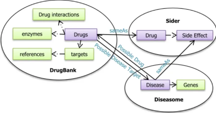
is a comprehensive knowledge base containing information about drugs, drug target (i.e. protein) information, interac-tions and enzymes. As it can be seen in Figure 1 the classes representing drugs in Drugbank and Sider are linked using
owl:sameAsand diseases from Diseasome are linked to drugs in Drugbank usingpossible Drug and possible Disease target. Diseases and side effects between Sider and Disea-some are linked using theowl:sameAs property. Note that in this figure the dotted arrows represent the properties be-tween classes inside a dataset.
Our approach can answer queries with the following three characteristics:
• Queries requiring fused information: An example is the query: “side effects of drugs used for Tubercu-losis”. Tuberculosis is defined in Diseasome, drugs for curing Tuberculosis are described in Drugbank, while we find their side effects in Sider.
• Queries targeting combined information: An ex-ample depicted in Figure 2 is the query: “side effect and enzymes of drugs used for ASTHMA”. Here the answer to that query can only be obtained by joining data from Sider (side effects) and Drugbank (enzymes, drugs).
• Query requiring keyword expansion: An exam-ple is the query “side effects of Valdecoxib”. Here the drug Valdecoxib can not be found in Sider, however, its synonym Bextra is available via Sider.
To the best of our knowledge our approach is the first ap-proach for answering questions on interlinked datasets by constructing a federated SPARQL query. Our main contri-butions can be summed up as follows:
• We extend the Hidden Markov Model approach for dis-ambiguating resources from different datasets. • We present a novel method for constructing formal
queries using disambiguated resources and leveraging the interlinking structure of the underlying datasets. • We developed a benchmark consisting of 25 queries
for a testbed in the life-sciences. The evaluation of our implementation demonstrates its feasibility with an f-measure of 90%.
This paper is organized as follows: In the subsequent sec-tion, we present the problem at hand in more detail and some of the notations and concepts used in this work. Sec-tion 3 presents the proposed disambiguaSec-tion method in de-tail along with the evaluation of the bootstrapping. In sec-tion 4, we then present the key steps of our algorithm for constructing a conjunctive query. Our evaluation results are presented in the section 5 while related work is reviewed in the section 6. We close with a discussion and future work.
2.
PROBLEM AND PRELIMINARIES
In this section, we introduce some crucial notions em-ployed throughout the paper and describe the main chal-lenges that arise when transforming user queries to formal, conjunctive queries on linked data.
Diseasome Sider
Drugs sameAs
Disease
Drug Side Effect
Genes enzymes
Drug interactions
references targets
DrugBank
Figure 1: Schema interlinking for three datasets i.e. DrugBank, Sider, Diseasome.
Diseasome
Drug
Asthma ?v0
side effect sameAs
a
?v2 ?v3
Disease
Drug Side Effect
a a
a
?v1 enzyme Enzymes
a
Sider DrugBank
Figure 2: Resources from three different datasets are fused at the instance level in order to exploit in-formation which are spread across diverse datasets.
An RDF knowledge base can be viewed as a directed, la-beled graph Gi = (Vi, Ei) where Vi is a set of nodes
com-prising all entities and literal property values, andEi is a
set of directed edges, i.e. the set of all properties. We define linked data in the context of this paper as a graph G= (V =S
Vi, E=SEi) containing a set of RDF
knowl-edge bases, which are linked to each other in the sense, that their sets of nodes overlap, i.e. thatVi∩Vj6=∅.
In this work we focus on user-supplied queries in natu-ral language, which we transform into an ordered sets of keywords by tokenizing, stop-word removal and lemmatiza-tion. Our input query thus is an n-tuple of keywords, i.e. Q= (k1, k2, ..., kn).
Challenge 1: Resource Disambiguation. In the first step, we aim to map the input keywords to a suitable set of entity identifiers, i.e. resourcesR ={r1, r2...rm}. Note,
that several adjacent keywords can be mapped to a single re-source, i.e. m≤n. In order to accomplish this task, the in-put keywords have to be grouped together to segments. For each segment, a suitable resource is then to be determined. The challenge here is to determine the right segment granu-larity, so that the most suitable mapping to identifiers in the underlying knowledge base can be retrieved for constructing a conjunctive query answering the input query.
For example, the question‘What is the side effects of drugs used for Tuberculosis?’ is transformed to the 4-keyword
tuple(side, effect, drug, Tuberculosis). This tuple can be segmented into (‘side effect drug’,‘Tuberculosis’) or (‘side effect’,‘drug’,‘Tuberculosis’). Note that the second segmen-tation is more likely to lead to a query that contains the re-sults intended by the user. In addition to detecting the right segments for a given input query, we also have to map each of these segments to a suitable resource in the underlying knowledge base. This step is dubbedentity disambiguation and is of increasing importance since the size of knowledge bases and schemes heterogeneity on the Linked Data Web grows steadily. In this example, the segment‘drug’ is am-biguous when querying both Sider and Diseasome because it may refer to the resourcediseasome:Tuberculosis describ-ing the disease Tuberculosis or to the resource
sider:Tuberculosisbeing the side effect caused by some drugs.
Challenge 2: Query Construction. Once the seg-mentation and disambiguation have been completed, ade-quate SPARQL queries have to be generated based on the detected resources. In order to generate a conjunctive query, a connected subgraphG0= (V0, E0) ofGcalled thequery graph has to be determined. The intuition behind con-structing such a query graph is that it has to fully cover the set of mapped resourcesR ={r1, ..., rm}while comprising
a minimal number of vertices and edges (|V0|
+|E0|). In
linked data, mapped resources ri may belong to different
graphsGi; thus the query construction algorithm must be
able to traverse the links between datasets at both schema and instance levels. With respect to the previous example, after applying disambiguation on the identified resources, we would obtain the following resources from different datasets:
sider:sideEffect,diseasome:possibleDrugand
diseasome:1154. The appropriate conjunctive query con-tains the following triple patterns:
1. diseasome:1154 diseasome:possibleDrug ?v1 .
2. ?v1 owl:sameAs ?v2 .
3. ?v2 sider:sideEffect ?v3 .
The second triple pattern bridges between the datasets Drug-bank and Sider.
2.1
Resource Disambiguation
In this section, we present the formal notations for ad-dressing the resource disambiguation challenge, aiming at mapping the n-tuple of keywordsQ= (k1, k2, ..., kn) to the
m-tuple of resourcesR= (r1, ..., rm).
Definition 1 (Segment and Segmentation). For a given query Q = (k1, k2, ..., kn), the segment S(i,j) is the sequence of keywords from start position i to end position j, i.e.,S(i,j)= (ki, ki+1, ..., kj). A query segmentation is an
m-tuple of segmentsSG(Q) = (S(0,i), S(i+1,j), ..., S(l,n))with non-overlapping segments arranged in a continuous order, i.e. for two continuous segmentsSx, Sx+1 :Start(Sx+1) =
End(Sx) + 1. The concatenation of segments belonging to a
segmentation forms the corresponding input queryQ.
Definition 2 (Resource Disambiguation). Let the seg-mentation SG0 = (S1(0,i), S
2
(i+1,j), ..., S x
(l,n)) be the suitable segmentation for the given query Q. Each segment Si of
SG0 is first mapped to a set of candidate resources Ri =
{r1, r2...rh}from the underlying knowledge base. The aim of
the disambiguation step is to detect an m-tuple of resources (r1, r2, ..., rm) ∈ R1×R2 ×. . .×Rm from the Cartesian
product of the sets of candidate resources for which eachri
Valid Segments Samples of Candidate Resources
side effect 1. sider:sideEffect 2. sider:side_effects
drug 1. drugbank:drugs 2. class:Offer
3. sider:drugs 4. diseasome:possibledrug
tuberculosis 1. diseases:1154 2. side_effects:C0041296
Table 1: Generated segments and samples of candi-date resources for a given query.
Data: q: n-tuple of keywords, knowledge base
Result: SegmentSet: Set of segments 1 SegmentSet=new list of segments; 2 start=1;
3 whilestart <=ndo
4 i=start;
5 while S(start,i)is validdo 6 SegmentSet.add(S(start,i));
7 i++;
8 end
9 start++;
10 end
Algorithm 1: Naive algorithm for determining all valid segments taking the order of keywords into account.
has two important properties: First, it is among the highest ranked candidates for the corresponding segment with respect to the similarity as well as popularity and second it shares a semantic relationship with other resources in the m-tuple. Semantic relationship refers to the existence of a path be-tween resources.
The disambiguated m-tuple is appropriate if a query graph [capable of answering the input query] can be constructed using all resources contained in that m-tuple. The order in which keywords appear in the original query is partially significant for mapping. However, once a mapping from key-words to resources is established the order of the resources does not affect the SPARQL query construction anymore. This is a fact that users will write strongly related keywords together, while the order of only loosely related keywords or keyword segments may vary. When considering the or-der of keywords, the number of segmentations for a query Qconsisting ofnkeywords is 2(n−1). However, not all these segmentations contain valid segments. A valid segment is a segment for which at least one matching resource can be found in the underlying knowledge base. Thus, the number of segmentations is reduced by excluding those containing invalid segments.
Algorithm 1 shows a naive approach for finding all valid segments when considering the order of keywords. It starts with the first keyword in the given query as first segment, then adds the next keyword to the current segment and checks whether this addition would render the new segment invalid. This process is repeated until we reach the end of the query. The input query is usually short. The number of keywords is mainly less than 64; therefore, this algorithm is not expensive. Table 1 shows the set of valid segments along with some samples of the candidate resources computed for the previous example using the naive algorithm. Note that ’side effect drug’, ’side’, ’effect’ are not a valid segments.
4
2.2
Construction of Conjunctive Queries
The second challenge addressed by this paper tackles the problem of generating a federated conjunctive query lever-aging the disambiguated resources i.e. R = (r1, ..., rm).Herein, we consider conjunctive queries being conjunctions of SPARQL algebra triple patterns5. We leverage the
disam-biguated resources and implicit knowledge about them (i.e. types of resources, interlinked instances and schema as well as domain and range of resources with the type property) to form the triple patterns.
For instance, for the running query which asks for a list of resources (i.e. side effects) which have a specific characteris-tic in common (i.e. caused by drugs used for Tuberculosis’). Suppose the resources identified during the disambiguation process are: sider:sideEffect, Diseasome:possibleDrug
as well asDiseasome:1154. Suitable triple patterns which are formed using the implicit knowledge are:
1. Diseasome:1154 Diseasome:possibleDrug ?v1 .
2. ?v1 owl:sameAs ?v2 .
3. ?v2 sider:sideEffect ?v3 .
The second triple pattern is formed based on interlinked data information. This triple connects the resources with the type drug in the dataset Drugbank to their equiva-lent resources with the typedrugin the Sider dataset using
owl:sameAslink. These triple patterns satisfy the informa-tion need expressed in the input query. Since most of com-mon queries comcom-monly lack of a quantifier, thus conjunctive queries to a large extend capture the user information need. A conjunctive query is called query graph and formally de-fined as follows.
Definition 3 (Query Graph). Let a set of resources R={r1, ..., rn}(from potentially different knowledge bases)
be given. A query graph QGR = (V0, E0) is a directed,
connected multi-graph such that R ⊆ E0∪V0. Each edge e ∈ E0 is a resource that represents a property from the underlying knowledge bases. Two nodes n and n0 ∈ V0 can be connected by e if n (resp. n0) satisfies the domain (resp. range) restrictions of e. Each query graph built by these means corresponds to a set of triple patterns. i.e.
QG≡ {(n, e, n0)|(n, n0
)∈V2∧e∈E}.
3.
RESOURCE DISAMBIGUATION USING
HIDDEN MARKOV MODELS
In this section we describe how we use a HMM for the concurrent segmentation of queries and disambiguation of resources. First, we introduce the notation of HMM param-eters and then we detail how we bootstrap the paramparam-eters of our HMM for solving the query segmentation and entity disambiguation problems.
Hidden Markov Models: Formally, a hidden Markov model (HMM) is a quintupleλ= (X, Y, A, B, π) where:
• X is a finite set of states. In our case,X is a subset of the resources contained in the underlying graphs. • Y denotes the set of observations. Herein,Y equals to
the valid segments derived from the input n-tuple of keywords.
5
Throughout the paper, we use the standard notions of the RDF and SPARQL specifications, such as graph pattern, triple pattern and RDF graph.
• A:X ×X →[0,1] is the transition matrix of which each entryaij= is the transition probabilityP r(Sj|Si)
from stateito statej;
• B : X ×Y → [0,1] represents the emission matrix. Each entrybih=P r(h|Si) is the probability of
emit-ting the symbolhfrom statei;
• π:X→[0,1] denotes the initial probability of states.
Commonly, estimating the hidden Markov model parame-ters is carried out by employing supervised learning. We rely onbootstrapping, a technique used to estimate an unknown probability distribution function. Specifically, we bootstrap6
the parameters of our HMM by using string similarity met-rics (i.e.,Levenshtein and Jaccard) for the emission proba-bility distribution and more importantly the topology of the graph for the transition probability. The results of the eval-uation show that by using these bootstrapped parameters, we achieve a mean reciprocal rank (MRR) above 84%.
Constructing the State Space: A-priori, the state space should be populated with as many states as there are entities in the knowledge base. The number of states inX is thus potentially large given thatX will contain all RDF resources contained in the graphG on which the search is to be carried out, i.e. X =V ∪E. For DBpedia, for ex-ample, X would contain more than 3 million states. To reduce the number of states, we exclude irrelevant states based on the following observations: (1) A relevant state is a state for which a valid segment can be observed (we described the recognition of valid segments in Section 2.1). (2) A valid segment is observed in a state if the probability of emitting that segment is higher than a given threshold θ. The probability of emitting a segment from a state is computed based on the similarity score which we describe in Section 3.1. Thus, we can prune the state space such that it contains solely the subset of the resources from the knowledge bases for which the emission probability is higher than θ. In addition to these states, we add an unknown entity state (UE) which represents all entities that were pruned. Based on this construction of state space, we are now able to detect likely segmentations and disambiguation of resources, the segmentation being the labels emitted by the elements of the most likely sequence of states. The dis-ambiguated resources are the states determined as the most likely sequence of states.
Extension of State Space with reasoning:A further extension of the state space can be carried out by including resources inferred from lightweight owl:sameAs reasoning. We precomputed and added the triples inferred from the symmetry and transitivity property of theowl:sameAs rela-tion. Consequently, for extending the state space, for each state representing a resourcexwe just include states for all resourcesy, which are in anowl:sameAsrelation withx.
3.1
Bootstrapping the Model Parameters
Our bootstrapping approach for the model parametersA andπis based on the HITS algorithm and semantic relations between resources in the knowledge base. The rationale is that the semantic relatedness of two resources can defined in
6For the bootstrapping test, we used 11 sample queries from
terms of two parameters: the distance between the two re-sources and the popularity of each of the rere-sources. The dis-tance between two resources is the path length between those resources. The popularity of a resource is simply the connec-tivity degree of the resource with other resources available in the state space. We use the HITS algorithm for transform-ing these two values to hub and authority values (as detailed below). An analysis of the bootstrapping shows significant improvement of accuracy due to this transformation. In the following, we first introduce theHITS algorithm, since it is employed within the functions for computing the two HMM parametersAandπ. Then, we discuss the distribution func-tions proposed for each parameter. Finally, we compare our bootstrapping method with other well-known distribution functions.
Hub and Authority of States. Hyperlink-Induced Topic Search (HITS) is a link analysis algorithm that was devel-oped originally for ranking Web pages [13]. It assigns a hub and authority value to each Web page. Thehub value es-timates the value of links to other pages and theauthority value estimates the value of the content on a page. Hub and authority values are mutually interdependent and com-puted in a series of iterations. In each iteration the authority value is updated to the sum of the hub scores of each refer-ring page; and the hub value is updated to the sum of the authority scores of each referring page. After each iteration, hub and authority values are normalized. This normaliza-tion process causes these values to converge eventually.
Since RDF data forms a graph of linked entities, we em-ploy a weighted version of the HITS algorithm in order to assign different popularity values to the states based on the distance between states. We compute the distance between states employing weighted edges. For each two statesSiand
Sj in the state space, we add an edge if there is a path of
maximum lengthkbetween the two corresponding resources. Note that we also takepropertyresources into account when computing the path length.The weight of the edge between the statesSi and Sj is set to wi,j =k−pathLength(i, j),
wherepathLength(i, j) is the length of the path between the corresponding resources. The authority of a state can now be computed by: auth(Sj) = P
Si
wi,j×hub(Si). The hub
value of a state is given byhub(Sj) = P Si
wi,j×auth(Si).
These definitions of hub and authority for states are the foundation for computing the transition and initial proba-bilities in the HMM.
Transition Probability. To compute the transition prob-ability between two states, we take both, the connectivity of the whole of space state as well as the weight of the edge be-tween the two states, into account. The transition probabil-ity value decreases with increasing distance between states. For example, transitions between entities in the same triple have a higher probability than transitions between entities in triples connected through auxiliary intermediate entities. In addition to edges representing the shortest path between en-tities, there is an edge between each state and theunknown entity (UE)state. The transition probability of stateSj
fol-lowing stateSiis denoted asaij=P r(Sj|Si). Note that the
conditionP Sj
P r(Sj|Si) = 1 holds.
The transition probability from the stateSito UE is
de-fined as:
aiU E=P r(U E|Si) = 1−hub(Si)
Consequently, a good hub has a smaller probability of tran-sition toUE. The transition probability from the stateSito
the stateSj is computed by:
aij=P r(Sj|Si) =
auth(Sj) P
∀aik>0
auth(Sk)
×hub(Si)
Here, the probability from stateSito the neighboring states
are uniformly distributed based on the authority values. Consequently, states with higher authority values are more probable to be met.
Initial Probability. The initial probabilityπ(Si) is the
probability that the model assigns to the initial stateSiin
the beginning. The initial probabilities fulfill the condition
P
∀Si
π(Si) = 1. We denote states for which the first keyword
is observable byInitialStates. The initial states are defined as follows:
π(Si) =
auth(Si) +hub(Si) P
∀Sj∈InitialStates
(auth(Sj) +hub(Sj))
In fact,π(Si) of an initial state is uniformly distributed on
both hub and authority values.
Emission Probability. Both the labels of states and the segments contain sets of words. For computing the emis-sion probability of the stateSi and the emitted segmenth,
we compare the similarity of the label of stateSi with the
segment h in two levels, namely string-similarity and set-similarity level:
• Thestring-similarity level measures the string similar-ity of each word in the segment with the most similar word in the label using theLevenshtein distance. • Theset-similarity levelmeasures the difference between
the label and the segment in terms of the number of words using theJaccard similarity.
Our similarity score is a combination of these two metrics. Consider the segment h = (ki, ki+1, ..., kj) and the words
from the labelldivided into a set of keywordsM and stop-wordsN, i.e.l=M∪N. The total similarity score between keywords of a segment and a label is then computed as fol-lows:
bih=P r(h|Si) = j P t=i
argmax
mi∈M
(σ(mi, kt))
|M∪h|+ 0.1∗ |N|
This formula is essentially an extension of theJaccard sim-ilarity coefficient. The difference is that we use the sum of the string-similarity score of the intersections in the numer-ator instead of the cardinality of intersections. As in the Jaccard similarity, the denominator comprises the cardinal-ity of the union of two sets (keywords and stopwords). The difference is that the number of stopwords is down-weighted by the factor 0.1 to reduce their influence since they do not convey much supplementary semantics.
Viterbi Algorithm for the K-best Set of Hidden States. The optimal path through the HMM for a given se-quence (i.e. input query keywords) generates disambiguated resources which form a correct segmentation. The Viterbi algorithm or Viterbi path [28] is a dynamic programming
approach for finding the optimal path through a HMM for a given input sequence. It discovers the most likely sequence of underlying hidden states that might have generated a given sequence of observations. This discovered path has the maximum joint emission and transition probability of the involved states. The sub-paths of this most likely path also have the maximum probability for the respective sub se-quence of observations. The naive version of this algorithm just keeps track of the most likely path. We extended this al-gorithm using a tree data structure to store all possible paths generating the observed query keywords. Thus, our imple-mentation can provide a ranked list of all paths generating the observation sequence with the corresponding probability. After running the Viterbi algorithm for our running exam-ple, the disambiguated resources are: {sider:sideEffect, dis-easome:possibleDrug, diseases:1154} and consequently the detected segmentation is: {side effect, drug, Tuberculosis}.
3.2
Evaluation of Bootstrapping
We evaluated the accuracy of our approximation of the transition probability A (which is basically a kind of uni-form distribution) in comparison with two other distribution functions, i.e.,Normal andZipfian distributions. Moreover, to measure the effectiveness of thehub and authority val-ues, we ran the distribution functions with two different in-puts, i.e. distance andconnectivity degree values as well as hub and authority values. Note that for a given edge the source state is the one from which the edge originates and the sink state is the one where the edge ends. We ran the distribution functions separately withXbeing defined as the weighted sum of the normalized distance between two states and normalized connectivity degree of the sink state:Xij=
α×distance(Si−Sj)+ (1−α)×(1−connectivityDegreeSj).
Similarly,Y was defined as the weighted sum of the hub of the source state and the authority of the sink state: Y = α×hub(Si) + (1−α)×(1−authorithysj). In addition,
to measuring the effectiveness ofhub andauthority, we also measured a similar uniform function with the input param-etersdistance andconnectivity degreedefined as:
aij=
distance(Si−Sj) P
∀Sk>0
distance(Si−Sk)
∗connectivitydegree(Si)
Given that the model at hand generates and scores a ranked list of possible tuples of resources, we compared the re-sults obtained with the different distributions by looking at themean reciprocal rank (MRR) [29] they achieve. For each queryqi∈Qin the benchmark, we compare the rank
ri assigned by different algorithms with the correct tuple
of resources and set M RR(A) = 1
|Q|
P qi
1
ri. Note that if
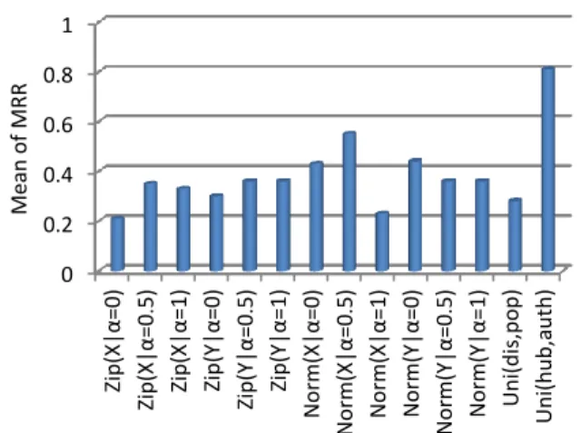
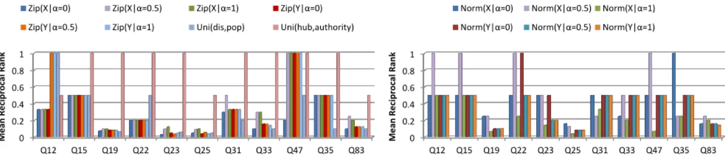
the correct tuple of resources was not found, the recipro-cal rank was assigned the value 0. We used 11 queries from QALD2-Benchmark 2012 training dataset for boot-strapping7. Figure 3 shows theM RRachieved by bootstrap-ping the transition probability of this model with 3 differ-ent distribution functions per query in 14 differdiffer-ent settings. Figure 4 compares the averageM RRfor different functions employed for bootstrapping the transition probability per setting. Our results show clearly that the proposed func-tion is superior to all other settings and achieves an MRR of approximately 81%. A comparison of the MRR achieved
7 http://www.sc.cit-ec.uni-bielefeld.de/qald-2 0 0.2 0.4 0.6 0.8 1 Zip(X| α =0 ) Zip(X| α =0 .5 ) Zip(X| α =1 ) Zip(Y| α =0 ) Zip(Y| α =0 .5 ) Zip(Y| α =1 ) Nor m( X| α =0 ) Nor m( X| α =0 .5 ) Nor m( X| α =1 ) Nor m( Y| α =0 ) Nor m( Y| α =0 .5 ) Nor m( Y| α =1 ) Uni(di s,pop) Uni(hub ,aut h) Mean of MRR
Figure 4: Comparison of different functions and set-tings for bootstrapping the transition probability. Uni stands for the uniform distribution, while Zip stands for the Zipfian and Norm for the normal dis-tribution.
when usinghubandauthority with that obtained when us-ing distance and connectivity degree reveals that usinghub andauthority leads to an 8% improvement on average. This difference is in Zipfian and Normal settings trivial, but very significant in the case of a uniform distribution. Essentially, HITS fairly assigns qualification values for the states based on the topology of the graph.
We bootstrapped the emission probabilityBwith two dis-tribution functions based on (1) Levenshtein similarity met-ric, (2) the proposed similarity metric as a combination of the Jaccard and Levenshtein measures. We observed the M RRachieved by bootstrapping the emission probability of this model employing those two similarity metrics per query in two settings (i.e. natural and reverse order of query key-words). The results show no difference in M RR between these two metrics in the natural order. However, in the reverse order the Levenshtein metric failed for 81% of the queries, while no failure was observed with the combination of Jaccard and Levenshtein. Hence, our combination is ro-bust with regard to change of input keyword order. For bootstrapping the initial probability π, we compared the uniform distribution on both – hub and authority – val-ues with a uniform distribution on the number of states for which the first keyword is observable. The result of this comparison shows a 5% improvement for the proposed func-tion. Figure 5 shows the mean ofM RRfor different values of the thresholdθemployed for prunning the state space. A high value ofθprevents inclusion of some relevant resources and a low value adds irrelevant resources. It can be observed that the optimal value of θis in the range [0.6,0.7]. Thus, we setθ to 0.7 in the rest of our experiments.
4.
QUERY GRAPH CONSTRUCTION
The goal of query graph construction is generating a con-junctive query (i.e. SPARQL query) from a given set of resource identifiers i.e., R = {r1, r2, ...rm}. The core of
SPARQL queries are basic graph patterns, which can be viewed as a query graph QG. In this section, we first dis-cuss the formal considerations underlying our query graph
0 0.2 0.4 0.6 0.8 1
Q12 Q15 Q19 Q22 Q23 Q25 Q31 Q33 Q47 Q35 Q83
Mean Reci
p
roc
al
Rank
Zip(X|α=0) Zip(X|α=0.5) Zip(X|α=1) Zip(Y|α=0) Zip(Y|α=0.5) Zip(Y|α=1) Uni(dis,pop) Uni(hub,authority)
0 0.2 0.4 0.6 0.8 1
Q12 Q15 Q19 Q22 Q23 Q25 Q31 Q33 Q47 Q35 Q83
Mean Reci
p
roc
al
Rank
Norm(X|α=0) Norm(X|α=0.5) Norm(X|α=1) Norm(Y|α=0) Norm(Y|α=0.5) Norm(Y|α=1)
Figure 3: MRR of different distributions per query for bootstrapping the transition probability.
0 0.2 0.4 0.6 0.8 1
0.1 0.2 0.3 0.4 0.5 0.6 0.7 0.8 0.9 1 1.1
M
ea
n
o
f
M
RR
Theta
Figure 5: Mean MRR for different values ofθ.
generation strategy and then describe our algorithm for gen-erating the query graph. The output of this algorithm is a set of graph templates. Each graph template represents a comprehensive set of query graphs, which are isomorphic re-garding edges. A query graphAis isomorphic regarding its edges to a query graph B, ifA can be derived fromB by changing the labels of edges.
4.1
Formal Considerations
A query graphQGconsists of a conjunction of triple pat-terns denoted by (si, pi, oi). When the set of resource
iden-tifiers R is given, we aim to generate a query graph QG satisfying the completeness restriction, i.e., each ri in R
maps to at least one resource in a triple pattern contained inQG. For a given set of resources R, the probability of a generated query graph Pr(QG|R) being relevant for an-swering the information need depends on the probability of all corresponding triple patterns to be relevant. We assume that triple patterns are independent with regard to the rele-vance probability. Thus, we define the relerele-vance probability for aQGas product of the relevance probabilities of then containing triple patterns. We denote the triple patterns with (si, pi, oi)i=1...n and their relevance probability with
Pr(si, pi, oi), thus rendering Pr(QG|R) =Qni=1Pr(si, pi, oi).
We aim at constructingQGwith the highest relevance
prob-ability, i.e.
arg max Pr(QG|R). There are two parameters that influ-ence Pr(QG|R): (1) the number of triple patterns and (2) the number of free variables, i.e. variables in a triple pat-tern that are not bound to any input resource. Given that ∀(si, pi, oi) : Pr(si, pi, oi) ≤1, a low number of triple
pat-terns increases the relevance probability ofQG. Thus, our approach aims at generating small query graphs to maxi-mize the relevance probability. Regarding the second pa-rameter, more free variables increase the uncertainty and consequently cause a decrease in Pr(QG|R). As a result of these considerations, we devise an algorithm that minimizes
the number of both the number of free variables and the number of triple patterns in QG. Note that is each triple pattern, the subjectsi(resp. objectoi) should be included
in the domain (resp. range) of the predicatepior be a
vari-able. Otherwise, we assume the relevance probability of the given triple pattern to be zero:
(si∈/domain(pi))∨(oi∈/range(pi))⇒Pr(si, pi, oi) = 0.
Forward Chaining. One of the prerequisites of our ap-proach is the inference of implicit knowledge on the types of resources as well as domain and range information of the properties. We define thecomprehensive type (CT) of a re-source r as the set of all super-classes of explicitly stated classes of r (i.e., those classes associated with r via the
rdf:typeproperty in the knowledge base). The comprehen-sive type of a resource can be easily computed using forward chaining on therdf:typeandrdfs:subClassOfstatements in the knowledge base. We can apply the same approach to properties to obtain maximal knowledge on their domain and range. We call the extended domain and range of a propertypcomprehensive domain(CDp) andcomprehensive
range(CRp). We reduce the task of finding the
comprehen-sive properties (CPr−r0) which link two resourcesr andr0
to finding propertiespsuch that the comprehensive domain (resp. comprehensive range) ofpintersects with the compre-hensive type ofrrespr0 or vice-versa. We call the setOPr
(resp. IPr) of all properties that can originate from (resp.
end with) a resourcerthe set of outgoing (resp. incoming) properties ofr.
4.2
Approach
To construct possible query graphs, we generate in a first step an incomplete query graph IQG(R) = (V00, E00) such that the vertices V00 (resp. edges E00) are either equal or subset of the vertices (resp. edges) of the final query graph V00 ⊆ V0 (resp. E00 ⊆ E0). In fact, an incomplete query graph (IQG) contains a set of disjoint sub-graphs, i.e. there is no vertex or edge in common between the sub-graphs:
IQG={gi(vi, ei)|∀gi6=gj:vi∩vj =∅ ∧ei∩ej =∅}. An
IQGconnects a maximal number of the resources detected beforehand in all possible combinations.
TheIQGis the input for the second step of our approach, which transforms the possibly incomplete query graphs into a set of final query graphsQG. Note that for the second step, we use an extension of the minimum spanning tree method that takes subgraphs (and not sets of nodes) as input and generates a minimal spanning graph as output. Since in the second step, the minimum spanning tree does not add any extra intermediate nodes (except nodes connected by
owl:sameAslinks), it eliminates both the need of keeping an index over the neighborhood of nodes and using exploration for finding paths between nodes.
Generation of IQGs.
After identifying a corresponding set of resources R = {r1, r2, ...rm}for the input query, we can construct vertices
V0 and primary edges of the query graph E00 ⊆ E0 in an initial step. Each resourceris processed as follows: (1) Ifr is an instance,CT of this vertex is equivalent toCT(r) and the label of this vertex isr. (2) Ifr is a class,CT of this vertex just containsrand the label of this vertex is a new variable.
After the generation of the vertices for all resources that are instances or classes, the remaining resources (i.e., the properties) generate an edge and zero (when connecting ex-isting vertices), one (when connecting an exex-isting with a new vertex) or two vertices. This step uses the sets of incoming and outgoing properties as computed by the forward chain-ing. For each resourcerrepresenting a property we proceed as follows:
• If there is a pair of vertices (v, v0) such thatrbelongs to the intersection of the set of outgoing properties of v and the set of incoming properties of v0 (i.e. r ∈ OPv∩IPv0), we generate an edge between v and v0
and label it with r. Note that in case several pairs (v, v0) satisfy this condition, an IQGis generated for each pair.
• Else, if there is a vertexv fulfilling the conditionr∈ OPv, then we generate a new vertexuwith the CTu
being equal to CRr and an edge labeled with the r
between those vertices (v, u). Also, if the condition r∈IPvforvholds, a new vertex wis generated with
CTwbeing equal toCDr as well as an edge betweenv
andwlabeled withr.
• If none of the above holds, two vertices are generated, one withCT equal toCDr and another one withCT
equal toCRr. Also, an edge between these two vertices
with labelris created.
This policy for generating vertices keeps the number of free variables at a minimum. Note that whenever a property is connected to a vertex, the associated CT of that vertex is updated to the intersection of the previousCT andCDp
(CRp respectively) of the property. Also, there may be
dif-ferent options for inserting a property between vertices. In this case, we construct an individualIQGfor each possible option. If the output of this step generates an IQG that contains one single graph, we can terminate as there is no need for further edges and nodes.
Example 1. We look at the query: What is the side
effects of drugs used for Tuberculosis?. Assume the
resource disambiguation process has identified the following resources:
1. diseasome:possibleDrug (type property)
CD={diseasome:disease}, CR={drugbank:drugs}
2. diseasome:1154 (type instance)
CT={diseasome:disease}
3. sider:sideEffect (type property)
CD={sider:drug}, CR={sider:sideeffect}
After running the IQGs generation, since we have only one resource with the typeclassorinstance, just one vertice is generated. Thereafter, since only the domain ofpossibleDrug
intersects with theCT of the node1154, we generate: (1) a new vertex labeled?v0with theCT being equal to
CR=drugbank:drugs, and (2) an edge labeledpossibleDrug
from1154 to ?v0. Since, there is no matched node for the property sideEffect we generate: (1) a new vertex labeled ?v1with theCTbeing equal tosider:drug, (2) a new vertex labeled ?v2with the CT being equal tosider:sideeffect, (3) an edge labeled sideEffect from?v1 to?v2. Figure 6 shows the constructedIQG, which contains two disjoint graphs.
1154 possibleDrug ?v0
Graph 1
?v1 sideEffect ?v2
Graph 2
Figure 6: IQGfor Example 1.
Connecting Sub-graphs of an IQG.
Since the query graphQGmust be a connected graph, we need to connect the disjoint sub-graphs in each of theIQGs. The core idea of our algorithm utilizes theMinimum Span-ning Tree(MST) approach, which builds a tree over a given graph connecting all the vertices. We use the idea behind Prim’s algorithm [3], which starts with all vertices and sub-sequently incrementally includes edges. However, instead of connecting vertices we connect individual disjoint sub-graphs. Hence, we try to find a minimum set of edges (i.e., properties) to span a set of disjoint graphs so as to obtain a connected graph. Therewith, we can generate a query graph that spans all vertices while keeping the number of vertices and edges at a minimum. Since a single graph may have many different spanning trees, there may be several query graphs that correspond to each IQG. We generate all dif-ferent spanning graphs because each one may represent a specific interpretation of the user query.
To connect two disjoint graphs we need to obtain edges that qualify for connecting a vertex in one graph with a suit-able vertex in the other graph. We obtain these properties by computing the set of comprehensive propertiesCP (cf. Section 4.1) for each combination of two vertices from ferent sub-graphs. Note that if two vertices are from dif-ferent datasets, we have to traverse owl:sameAs links to compute a comprehensive set of properties. This step is crucial for constructing a federated query over interlinked data. In order to do so, we first retrieve the direct prop-erties between two vertices?v0 ?p ?v1.In case such prop-erties exist, we add an edge between those two vertices to IQG. Then, we retrieve the properties connecting two ver-tices via an owl:sameAs link. To do that, we employ two graph patterns: (1) ?v0 owl:sameAs ?x. ?x ?p ?v1. (2)
?v0 ?p ?x. ?x owl:sameAs ?v1.The resulting matches to each of these two patterns are added to theIQG. Finally, we obtain properties connecting vertices havingowl:sameAs
links according to the following pattern:
?v0 owl:sameAs ?x. ?x ?p ?y. ?y owl:sameAs ?v1.Also, matches for this pattern are added to theIQG.
For each connection discovered between a pair of vertices (v, v0), a different IQGis constructed by adding the found edge connecting those vertices to the original IQG. Note that the IQGresulting from this process contains less un-connected graphs than the inputIQG. The time complexity
in the worst case is O(|v|2) (with |v| being the number of
vertices).
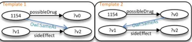
Example 2. To connect two disjoint graphs i.e. Graph 1 and Graph 2 of the IQG shown in Example 1, we need to obtain edges that qualify for connecting either the ver-tex 1154 or ?v0 to either vertex ?v1 or ?v2 in Graph 2. Forward chaining reveals the existence of two owl:sameAs
connections between two vertices i.e. (1)1154and?v2, (2) ?v0 and ?v1. Therefore, we can construct the first query graph template by adding an edge between1154and?v2and the second query graph template by adding an edge between ?v0 and?v1. The two generated query graph templates are depicted in Figure 7.
1154 possibleDrug ?v0
Template 1
?v1 ?v2
sideEffect
Template 2
1154 possibleDrug ?v0
?v1 ?v2
sideEffect
Figure 7: Generated query graph templates.
Our approach was implemented as a Java Web application which is publicly available athttp://sina-linkeddata.aksw. org. The algorithm is knowledge-base-agnostic and can thus be easily used with other knowledge bases.
5.
EVALUATION
Experimental Setup.
The goal of our evaluation was to determine how well (1) our resource disambiguation and (2) our query construc-tion approaches perform. To the best of our knowledge, no benchmark for federated queries over Linked Data has been created so far. Thus, we created a benchmark of 25 queries on the 3 interlinked datasets Drugbank, Sider and Disea-some for the purposes of our evaluation8. The benchmark
was created by three independent SPARQL experts, which provided us with (1) a natural-language query and (2) the equivalent conjunctive SPARQL query. We selected these three datasets because they are a fragment of the well inter-linked biomedical fraction of the Linked Open Data Cloud9 and thus represent an ideal case for the future structure of Linked Data sources.
We measured the performance of our resource disambigua-tion approach using theMean Reciprocal Rank(MRR). More-over, we measured the accuracy of the query construction in terms of precision and recall. To compute the precision, we compared the results returned from the query construction method with the results of the reference query provided by the benchmark. The query construction is initiated with the top-1 tuple returned by the disambiguation approach. All experiments were carried out on a Windows 7 machine with an Intel Core2 Duo (2.66GHz) processor and 4GB of RAM. For testing the statistical significance of our results, we used a Wilcoxon signed ranked test with a significance level of 95%.
8The benchmark queries are available athttp://aksw.org/ Projects/lodquery
9E.g., 859 owl:sameAs links exists between the 924 drug
instances in Sider and the 4772 drug instances in Drugbank
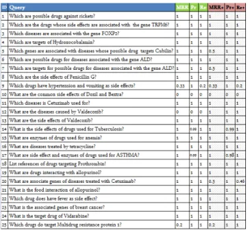
Results.
The detailed results of our evaluation are shown in Fig-ure 9. We ran our approach without and with OWL inferenc-ing durinferenc-ing the state space construction. When ran without inferencing, our approach was able to disambiguate 23 out of 25 (i.e. 92%) of the resources contained in the queries without mistakes. For Q9 (resp. Q25), the correct disam-biguation was only ranked third (resp. fifth). In the other two cases (i.e. Q10 and Q12), our approach simply failed to retrieve the correct disambiguation. This was due to the path between Doxil and Bextra not being found for Q10 as well as the mapping from disease to side effectnot being used in Q12. Overall, we achieve an MRR of 86.1% without inferencing. The MRR was 2% lower (not statis-tically significant) when including OWL inferencing due to the best resource disambiguation being ranked at the second position for three queries that were disambiguated correctly without inferencing (Q5, Q7 and Q20). This was simply due to the state space being larger and leading to higher tran-sition probabilities for the selected resources. With respect to precision and recall achieved with and without reason-ing, there were also no statistically significant differences between the two approaches. The approach without reason-ing achieved a precision of 0.91 and a recall of 0.88 while using reasoning led to precision (resp. recall) values of 0.95 (resp. 0.90). Although performance was not (yet) the pri-mary focus of our work, we want to provide evidence, that our approach can be used for real-time querying. Overall the pros and cons of using inferencing are clearly illustrated in the results of our experiments. On Q12, our approach is unable to construct a query without reasoning due to the missing equivalence between the terms disease and side effect. This equivalence is made available by the inference engine, thus making the construction of the SPARQL query possible. On the downside, adding supplementary informa-tion through inferencing alters the ranking of queries and can thus lead to poorer recall values as in the case of Q20.
Figure 8 shows the runtime average of disambiguation and query construction with and without inferencing during the state space construction for three runs. As it can be ex-pected, inferencing increases the runtime, especially when the number of input keywords is high. Despite carrying out all computations on-the-fly, disambiguation and query con-struction terminate in reasonable time, especially for smaller number of keywords. After implementing further perfor-mance optimizations (e.g. indexing resource distances), we expect our implementation to terminate in less than 10s also for up to 5 keywords.
6.
RELATED WORK
Severalinformation retrieval and question answer-ingapproaches have been developed for the Semantic Web over the past years. Most of these approaches are adapta-tions of document retrieval approaches. Swoogle [5], Wat-son [4] andSindice[24], for example, stick to the document-centric paradigm. Recently, entity-document-centric approaches, such asSig.Ma[23],Falcons[2],SWSE[11], have emerged. How-ever, the basis for all these services are keyword indexing and retrieval relying on the matching user keywords and indexed terms. Examples of question answering systems are PowerAqua [16] andOntoNL[12]. PowerAqua can au-tomatically combine information from multiple knowledge bases at runtime. The input is a natural language query
1 10 100
2 3 4 5 6
avg
ru
n
time
(s)
Number of Keywords
Disambiguation Disambiguation+ QueryConstruction QueryConstruction+
Figure 8: Average runtime of disambiguation and query construction with (+) and without reasoning in the disambiguation phase in logarithmic scale.
and the output is a list of relevant entities. PowerAqua lacks a deep linguistic analysis and can not handle complex queries.Pythia[26] is a question answering system that em-ploys deep linguistic analysis. It can handle linguistically complex questions, but is highly dependent on a manually created lexicon. Therefore, it fails with datasets for which the lexicon was not designed. Pythia was recently used as kernel forTBSL[25], a more flexible question-answering sys-tem that combines Pythia’s linguistic analysis and theBOA framework [7] for detecting properties to natural language patterns. Exploring schema from anchor points bound to in-put keywords is another approach discussed in [22]. Query-ing Linked datasets is addressed with the work mainly treat both the data and queries as bags of words [2, 30]. [10] presents a hybrid solution for querying linked datasets. It run the input query against one particular dataset regard-ing the structure of data, then for candidate answers, it finds and ranks the linked entities from other datasets . Our ap-proach is a prior work as it queries all the datasets at hand and then according to the structure of the data, it makes a federated query. Furthermore, our approach is independent of any linguistic analysis and does not fail when the input query is an incomplete sentence.
Segmentation and disambiguationare inherent chal-lenges of keyword-based search. Keyword queries are usu-ally short and lead to significant keyword ambiguity [27]. Segmentation has been studied extensively in the natural language processing (NLP) literature e.g., [18]). NLP tech-niques for chunking such as part-of-speech tagging or name entity recognition cannot achieve high performance when applied to query segmentation. [17] addresses the segmen-tation problem as well as spelling correction and employs a dynamic programming algorithm based on a scoring func-tion for segmentafunc-tion and cleaning. An unsupervised ap-proach to query segmentation in Web search is described in [21]. [32] is a supervised method based on Conditional Ran-dom Fields (CRF) whose parameters are learned from query logs. For detecting named entities, [9] uses query log data and Latent Dirichlet Allocation. In addition to query logs, various external resources such as Web pages, search result
Figure 9: Accuracy results for the benchmark.
snippets, Wikipedia titles and a history of the user activi-ties have been used [19, 21, 1, 20]. Still, the most common approach is using the context for disambiguation [15, 6, 14]. In this work, resource disambiguation is based on the struc-ture of the knowledge at hand as well as semantic relations between the candidate resources mapped to the keywords of the input query.
7.
DISCUSSION AND CONCLUSION
We presented a two-step approach for question answer-ing from user-supplied queries over federated RDF data. A main assumption of this work is that some schema infor-mation is available for the underlying knowledge base and resources are typed according to the schema. Regarding the disambiguation, the superiority of our model is related to the transition probabilities. We achieved a fair balance be-tween the qualification of states for transiting by reflecting the popularity and distance in the hub and authority values and setting a transition probability to the unknown entity state (depending on the hub value). This resulted in an ac-curacy of the generated answers of more than 90% for our test-bed with life-science datasets. This work represents a first step in a larger research agenda aiming to make the whole Data Web easily queryable. For scaling the imple-mentation, a first avenue of improvements is related to the performance of the system, which can be improved by sev-eral orders of magnitued thorough including better indexing and precomputed forward-chaining.
Acknowledgments
We would like to thank our colleagues from AKSW research group for their helpful comments and inspiring discussions during the development of this approach. This work was supported by a grant from the European Union’s 7th Frame-work Programme provided for the project LOD2 (GA no. 257943).
8.
REFERENCES
[1] D. J. Brenes, D. Gayo-Avello, and R. Garcia. On the fly query entity decomposition using snippets.CoRR, abs/1005.5516, 2010.
[2] Gong Cheng and Yuzhong Qu. Searching linked objects with falcons: Approach, implementation and evaluation.Int. J. Semantic Web Inf. Syst.,
5(3):49–70, 2009.
[3] David R. Cheriton and Robert Endre Tarjan. Finding minimum spanning trees.SIAM J. Comput., 1976. [4] M. D’aquin, E. Motta, M. Sabou, S. Angeletou,
L. Gridinoc, V. Lopez, and D. Guidi. Toward a new generation of semantic web applications.Intelligent Systems, IEEE, 23(3):20–28, 2008.
[5] Li Ding, Timothy W. Finin, Anupam Joshi, Rong Pan, R. Scott Cost, Yun Peng, Pavan Reddivari, Vishal Doshi, and Joel Sachs. Swoogle: a search and metadata engine for the semantic web. InCIKM. ACM, 2004.
[6] L. Finkelstein, E. Gabrilovich, Y. Matias, E. Rivlin, Z. Solan, G. Wolfman, and E. Ruppin. Placing Search in Context: the Concept Revisited. InWWW, 2001. [7] Daniel Gerber and Axel-Cyrille Ngonga Ngomo.
Extracting multilingual natural-language patterns for rdf predicates. InProceedings of EKAW, 2012. [8] K.I. Goh, M.E. Cusick, D. Valle, B. Childs, M. Vidal,
and A.L. Barab´asi. Human diseasome: A complex network approach of human diseases. InAbstract Book of the XXIII IUPAP International Conference on Statistical Physics. 2007.
[9] J. Guo, G. Xu, X. Cheng, and H. Li. Named entity recognition in query. ACM, 2009.
[10] Daniel M. Herzig and Thanh Tran. Heterogeneous web data search using relevance-based on the fly data integration. pages 141–150. ACM, 2012.
[11] Aidan Hogan, Andreas Harth, J ˜Aijrgen Umbrich, Sheila Kinsella, Axel Polleres, and Stefan Decker. Searching and browsing linked data with swse: The semantic web search engine.J. Web Sem., 9(4), 2011. [12] Anastasia Karanastasi, Alexandros Zotos, and Stavros
Christodoulakis. The OntoNL framework for natural language interface generation and a domain-specific application. InFirst International DELOS
Conference, Pisa, Italy. 2007.
[13] J. M. Kleinberg. Authoritative sources in a hyperlinked environment.J. ACM, 46(5), 1999. [14] R. Kraft, C. C. Chang, F. Maghoul, and R. Kumar.
Searching with context. InWWW ’06. ACM, 2006. [15] S. Lawrence. Context in web search.IEEE Data Eng.
Bull., 23(3):25–32, 2000.
[16] V. Lopez, Fernandez M., Motta E., and N. Stieler. Poweraqua: Supporting users in querying and exploring the semantic web. InJournal of Semantic Web, In press.
[17] K. Q. Pu and X. Yu. Keyword query cleaning. PVLDB, 1(1):909–920, 2008.
[18] Lance A. Ramshaw and Mitchell P. Marcus. Text chunking using transformation-based learning.CoRR, 1995.
[19] K. M. Risvik, T. Mikolajewski, and P. Boros. Query segmentation for web search. 2003.
[20] A. Shepitsen, J. Gemmell, B. Mobasher, and R. Burke. Personalized recommendation in social tagging systems using hierarchical clustering. ACM, 2008. [21] B. Tan and F. Peng. Unsupervised query segmentation
using generative language models and wikipedia. In WWW. ACM, 2008.
[22] Thanh Tran, Haofen Wang, Sebastian Rudolph, and Philipp Cimiano. Top-k exploration of query candidates for efficient keyword search on graph-shaped (rdf) data. InICDE, 2009.
[23] Giovanni Tummarello, Richard Cyganiak, Michele Catasta, Szymon Danielczyk, Renaud Delbru, and Stefan Decker. Sig.ma: Live views on the web of data. J. Web Sem., 8(4):355–364, 2010.
[24] Giovanni Tummarello, Renaud Delbru, and Eyal Oren. Sindice.com: weaving the open linked data. 2007. [25] Christina Unger, Lorenz B¨uhmann, Jens Lehmann,
Axel-Cyrille Ngonga Ngomo, Daniel Gerber, and Philipp Cimiano. Template-based question answering over rdf data. ACM, 2012.
[26] Christina Unger and Philipp Cimiano. Pythia: compositional meaning construction for
ontology-based question answering on the semantic web. In16th Int. Conf. on NLP and IS, NLDB’11, pages 153–160, 2011.
[27] A. Uzuner, B. Katz, and D. Yuret. Word sense disambiguation for information retrieval. AAAI Press, 1999.
[28] Andrew J. Viterbi. Error bounds for convolutional codes and an asymptotically optimum decoding algorithm.IEEE Transactions on Information Theory, IT-13(2), 1967.
[29] E. Vorhees. The trec-8 question answering track report. InProceedings of TREC-8, 1999.
[30] Haofen Wang, Qiaoling Liu, Thomas Penin, Linyun Fu, Lei Zhang 0007, Thanh Tran, Yong Yu, and Yue Pan. Semplore: A scalable ir approach to search the web of data.J. Web Sem., 2009.
[31] David S. Wishart, Craig Knox, Anchi Guo, Savita Shrivastava, Murtaza Hassanali, Paul Stothard, Zhan Chang, and Jennifer Woolsey. Drugbank: a
comprehensive resource for in silico drug discovery and exploration.Nucleic Acids Research,
34(Database-Issue), 2006.
[32] X. Yu and H. Shi. Query segmentation using conditional random fields. ACM, 2009.