397
[Journal of Political Economy,2004, vol. 112, no. 2]
䉷2004 by The University of Chicago. All rights reserved. 0022-3808/2004/11202-0002$10.00
Do the Rich Save More?
Karen E. Dynan
Federal Reserve Board
Jonathan Skinner
Dartmouth College and National Bureau of Economic Research
Stephen P. Zeldes
Columbia University and National Bureau of Economic Research
The question of whether higher–lifetime income households save a larger fraction of their income was the subject of much debate in the 1950s and 1960s, and while not resolved, it remains central to the evaluation of tax and macroeconomic policies. We resolve this long-standing question using new empirical methods applied to the Panel Study of Income Dynamics, the Survey of Consumer Finances, and the Consumer Expenditure Survey. We find a strong positive rela-tionship between saving rates and lifetime income and a weaker but still positive relationship between the marginal propensity to save and lifetime income. There is little support for theories that seek to explain these positive correlations by relying solely on time preference rates, We thank Dan Bergstresser, Jeffrey Brown, Wynn Huang, Julie Kozack, Geng Li, Stephen Lin, Byron Lutz, and Marta Noguer for research assistance; Orazio Attanasio for help with the CEX data; Joe Lupton for help with the PSID data; and Andrew Samwick for help with the Social Security data and calculations. Zeldes is grateful for financial support from Columbia Business School and a TIAA-CREF Pension and Economic Research grant, and Skinner for financial assistance from the National Institute on Aging (PO1 AG19783). We thank two anonymous referees, Don Fullerton, David Laibson, Steve Levitt, James Poterba, John Sabelhaus, James Smith, Mark Warshawsky, David Weil, and seminar participants at the NBER Summer Institute, the NBER Inter-American Conference, the Universities of Michigan, Maryland, Pennsylvania, California at Berkeley, Chicago, Georgetown, Harvard, Johns Hopkins, Northwestern, New York, Stanford, and Yale for helpful comments; we are especially grateful to Casey Mulligan for detailed suggestions. The views expressed are those of the authors and not necessarily those of the Federal Reserve Board or its staff.
nonhomothetic preferences, or variations in Social Security benefits. There is more support for models emphasizing uncertainty with re-spect to income and health expenses, bequest motives, and asset-based means testing or behavioral factors causing minimal saving rates among low-income households.
I. Introduction
It would be easy to convince a room full of noneconomists that higher lifetime income levels lead to higher saving rates. Noneconomists would tell you that low-income people cannot afford to save. Certainly a room full of journalists would need little convincing: Examples include “a sales tax would shift the tax burden from the rich to the middle class, since affluent people save a much larger portion of their earnings” (Passell 1995, p. 1) and “the poor and middle class spend a higher percentage of their income on goods than do the rich, and so, according to most economists’ studies, a value-added tax is regressive” (Green-house 1992, p. 1).
A room full of economists would be less easily persuaded that higher lifetime income levels lead to higher saving rates. The typical economist would point out that people with temporarily high income will tend to save more to compensate for lower future income, and people with temporarily low income will tend to save less in anticipation of higher future income. Thus, even if the saving rate is invariant with regard to lifetimeincome, we would observe people with highcurrentincomes sav-ing more than their lower-income brethren (Friedman 1957).
Moreover, one can point to several stylized facts that do not seem to support a positive correlation between saving rates and income. First, there has been no time-series increase in the aggregate saving rate dur-ing the past century despite dramatic growth in real per capita income. Also, the increasing concentration of income toward the top income quintile during the 1980s and early 1990s did not lead to higher ag-gregate saving rates.1
Looking across countries, Schmidt-Hebbel and Serven (2000) found no evidence of a statistically significant link be-tween measures of income inequality and aggregate saving rates. Turn-ing to household data, several recent studies that estimate roughly con-stant wealth-income ratios across lifetime income groups (Gustman and Steinmeier 1997, 1999; Venti and Wise 1999) pose a serious challenge to the view that saving rates rise with lifetime income.
1Blinder (1975) finds little connection between shifts in the income distribution and
the aggregate saving rate but argues that the changes in the income distribution present in postwar U.S. data are unlikely to correspond to the type of pure redistribution required by the theory.
Despite an outpouring of research in the 1950s and 1960s, the ques-tion of whether the rich save more has since received little attenques-tion. Much of the early empirical work favored the view that high-income people did in fact save a higher fraction of their income (e.g., Mayer 1966, 1972). However, studies by Milton Friedman and others that reached the opposite conclusion, together with suggestive evidence like that described above, have left “reasonable doubt” about the alleged propensity of high–lifetime income households to save more.
We return to the relationship between saving rates and lifetime in-come for two reasons. First, there are a wide variety of newer data sources such as the Panel Study of Income Dynamics (PSID), the Survey of Consumer Finances (SCF), the Consumer Expenditure Survey (CEX), and work on imputed saving from Social Security and pension contri-butions (Gustman and Steinmeier 1989; Feldstein and Samwick 1992). Second, we believe that the topic has important implications for the evaluation of economic policy. If Friedman and his collaborators did not earn a clear-cut victory in the empirical battles of the 1960s, they won the war. “Representative agent” models and many other models used for macroeconomic or microeconomic policy evaluation assume that saving rates are at best invariant to proportional increases in the sum of human and physical wealth (Auerbach and Kotlikoff 1987; Ful-lerton and Rogers 1993; Leeper and Sims 1994; Altig et al. 2001).
The link between income and saving rates bears on a number of specific issues. First, differences across income groups in saving rates and marginal propensities to save imply that the effects on aggregate consumption of shocks to aggregate income or wealth depend on the distribution of the shock across income groups (see Stoker 1986; Shapiro and Slemrod 2003); this issue figured prominently in the debate sur-rounding the 2001 tax “rebates.” Second, the incidence and effectiveness of reform proposals that shift taxation away from saving, such as con-sumption or value-added taxes or expanded 401(k) or individual re-tirement accounts, depend on how much saving is done by each income group. Third, the link between income and saving rates influences how changes in income inequality alter saving and possibly aggregate growth. Finally, the question of whether higher-income households save at higher rates than lower-income households has important implications for the distribution of wealth.
We find first, like previous researchers, a strong positive relationship between current income and saving rates across all income groups, in-cluding the very highest income categories. Second, and more impor-tant, we continue to find a positive correlation when we use proxies for permanent income such as education, lagged and future earnings, and measures of consumption. Estimated saving rates range from zero for the bottom quintile of the income distribution to more than 25 percent
of income for the top quintile. The positive relationship is equally strong or even more pronounced when we include imputed Social Security saving and pension contributions. Among the elderly, we find little ev-idence of dissaving and some suggestive evev-idence of slightly higher sav-ing rates among high-income households. In sum, our results suggest strongly that the rich do save more; more broadly, we find that saving rates increase across the entire income distribution. In addition, we present evidence suggesting that the marginal propensity to save is greater for higher-income households than for lower-income house-holds.
After documenting the basic patterns of saving, we consider why the rich save more. Our findings are not consistent with the predictions of standard homothetic life cycle models. Nor, as we show below, are they consistent with explanations that range from differences in time pref-erence rates or subsistence parameters to variation in Social Security replacement rates. Alternative models of saving that can explain the empirical regularities include those with hyperbolic discounting (e.g., Laibson, Repetto, and Tobacman 1998) or those with differential asset accumulation against out-of-pocket health expenditures late in life (e.g., Smith 1999b; Dynan, Skinner, and Zeldes 2002).
II. The Empirical and Theoretical Background
Many economists in previous generations used both theory and empirics to assess whether people with high incomes save more than those with low incomes (e.g., Fisher 1930; Keynes 1936; Vickrey 1947; Duesenberry 1949; Hicks 1950; Pigou 1951; Friend and Kravis 1957; Modigliani and Ando 1960). In his pioneering work on the permanent income hy-pothesis, Friedman (1957) argued that the positive correlation between income and saving rates observed in cross-sectional data reflected in-dividuals changing their saving in order to keep consumption smooth in the face of temporarily high or low income. He presented empirical evidence consistent with the proportionality hypothesis that individuals with high permanent income consume the same fraction of income as individuals with low permanent income. Many studies of this hypothesis followed, some supporting Friedman and some not. Evans (1969) sum-marized the state of knowledge about consumption in 1969, concluding that “it is still an open question whether relatively wealthy individuals save a greater proportion of their income than do relatively poor in-dividuals” (p. 14).
In a comprehensive examination of the available results and data, Mayer (1972) disagreed, claiming strong evidence against the propor-tionality hypothesis. For example, using five-year income and spending measures, he found the elasticity of consumption with respect to
per-manent income to be significantly below one (0.905) and not much different from the elasticity based on one year of income.
Despite the abundance of early studies on this important question, little work has been done since the 1970s. The lull in part reflects the influential work of Lucas (1976) and Hall (1978), which shifted interest away from learning about levels of consumption or saving and toward “Euler equation” estimation techniques that implicitly examine first dif-ferences in consumption (see Browning and Lusardi 1996).
Some studies have found that wealth levels are disproportionately higher among households with high lifetime income (Diamond and Hausman 1984; Bernheim and Scholz 1993; Hubbard, Skinner, and Zeldes 1995). While this result could be explained by higher saving rates among higher-income households, it could also be explained by higher rates of return (on housing or the stock market, e.g.) or the receipt of proportionately more intergenerational transfers by these households. Others (Gustman and Steinmeier 1999; Venti and Wise 1999) have ar-gued that ratios of wealth including Social Security and pension wealth to lifetime income are no higher among high-income households, con-sistent with the Friedman hypothesis.
To help make our question more precise, consider a life cycle/per-manent income model with a bequest motive. At each aget, households maximize expected lifetime utility
T ∗
U(Cis)Dis
U {E
冘
⫹(D ⫺D)V(B ) , (1)it t
[
(1⫹d)s⫺t is⫺1 is is]
spt iwhereEis the expectation operator,Cis∗is nonmedical consumption for householdiat ages,diis the household-specific rate of time preference, is the bequest left in the event of death, and is the utility of
Bis V(7)
leaving a bequest. To allow for mortality risk,Disis a state variable that is equal to one if the household is alive through period s and zero otherwise, andTis the maximum possible length of life.
The family begins periodswith net worth (exclusive of human wealth) , where is the real after-tax rate of return on non– Ais⫺1(1⫹ris⫺1) ris⫺1
human wealth betweens⫺1ands. We assume that there are no private annuity markets. The family first learns about medical expenses(Mis), which we treat as necessary consumption that generates no utility. It next receives transfers (TRis) from the government. It then learns whether it survives through the period. If not, it leaves to heirs a non-negative bequest
B pA (1⫹r )⫺M ⫹TR . (2)
is is⫺1 is⫺1 is is
nonmedical consumption. We define total consumption asC {C∗⫹
is is . End-of-period wealth is thus
Mis (Ais)
A pA (1⫹r )⫹TR ⫹E ⫺C . (3)
is is⫺1 is⫺1 is is is
We define real annual income asY {r A ⫹E ⫹TR and saving is is⫺1 is⫺1 is is
asS {Y ⫺C pA ⫺A .2 is is is is is⫺1
Define lifetime resources (as of age t) as age t non–human wealth plus the expected present value of future earnings and transfers. Under what circumstances will saving rates be identical across households with different lifetime resources? In a life cycle model without uncertainty, there are two alternative assumptions that will cause consumption to be proportional to lifetime resources. Either we can assume that the rate of time preference (di) and the rate of return(ris)are constant and equal to each other (in which case the result holds for any time-separable utility function), or we can assume that preferences are homothetic (i.e., , in which case the result holds for any rate 1⫺g
U(C)p[C ⫺1]/[1⫺g]
of interest or time preference). If all households face the same interest rates and have the same preference parameters and life span, then the ratio of consumption to lifetime resources will be the same for all house-holds (of a given age). If one further assumes that the initial wealth and the age-earnings and age-transfers profiles of rich households are simply scaled-up versions of those for poor households, then the pro-portionality in consumption implies that the saving rate (at a given age) will be the same across lifetime resource groups.3
How then could saving rates differ across income groups? We consider three general classes of models: one encompasses certainty models with-out a bequest motive, the second allows for uncertainty with respect to future income or health expenses (but no bequest motive), and the third includes an operative bequest motive. To provide illustrative cal-culations of how saving rates differ across income groups in these classes of models, we present results from a simple three-period version of the model above. We think of period 1 (“young”) as ages 30–60, period 2
2Note that sincerincludes the total return to non–human wealth including capital
gains, saving measured as income minus consumption is identical to saving measured as the change in wealth. We return to this issue below.
3Adding uncertainty complicates the model, but again two sets of assumptions will
generate the result that consumption rises proportionately with the scale factor for earn-ings. First, if the utility function is quadratic anddiandrisare constant and equal to each
other, consumption will be proportional to the expected value of lifetime resources, as defined above. If the utility function is not quadratic, then there is no single summary statistic that defines consumption. However, if one assumes that the utility function is isoelastic and initial wealth and all possible realizations of earnings are scaled up by a constant factor, then consumption will also be scaled up by that factor and saving rates will be identical (Bar-Ilan 1995).
(“old”) as ages 60–90, and period 3 as the time around death (when old) when medical expenditures are paid and bequests are left.4
A. Consumption Models with No Uncertainty and No Bequest Motive We begin with a model with no bequest motive and no uncertainty other than about the length of life.5We use an isoelastic utility function with , a value consistent with previous studies. We examine low-income
gp3
and high-income groups, with respective average first-period incomes of $14,634 and $78,666, based on the top and bottom quintiles of five-year average income from the 1984–89 PSID (discussed in more detail below). We assume that in the second period Social Security and pension income replace 60 percent of preretirement (or first-period) income, consistent with the overall replacement rate in Gustman and Steinmeier (1999). The (annual) rates of time preference and interest are 0.02 and 0.03, respectively, which, together with uncertain life span, result in a roughly flat pattern of nonmedical consumption over the lifetime.
As shown in table 1, for both working-age (young) and retirement age (old) households, the predicted saving rate for the low-income group is identical to that of the high-income group. The saving rate (exclusive of pension and Social Security) while young equals 12.5 per-cent and while old equals⫺16.0 percent.
There are two approaches to generating higher saving rates for higher-income households in the standard life cycle model: differences in the timing of income for these households and differences in the timing of consumption. We consider each in turn.
Differences in the timing of earnings and transfers across lifetime income groups do not change the slope of the consumption path but yield different patterns of saving. For example, Social Security programs typically provide a higher replacement rate for low-income households and thus reduce the need for these households to save for retirement (e.g., Smith 1999b; Huggett and Ventura 2000).6As shown in table 1, increasing the replacement rate for the low-income households from 60 percent to 75 percent (and increasing their first-period Social Se-curity taxes such that the present value of lifetime resources is unaf-fected) reduces saving while young—to 6.7 percent. However, it also increases saving while old to⫺7.5 percent. The higher replacement rate
4
The only purpose of the third period is to allow for medical expenses late in life; we assume no nonmedical consumption in this period.
5We set the probability of living to old age (period 2) at 82 percent, on the basis of
U.S. life tables from the Berkeley-Wilmoth data set (http://www.demog.berkeley.edu/ wilmoth/mortality/). Since period 3 represents the very end of life, all households that survive to period 2 die in period 3.
6Other examples include differences in age-earnings profiles, differences in life
TABLE 1
Simulated Saving Patterns Saving Rate of
Young
Saving Rate of Old Benchmark:
Low income 12.5 ⫺16.0
High income 12.5 ⫺16.0
Income replacement rate:
Low income (75%) 6.7 ⫺7.5
High income (60%) 12.5 ⫺16.0
Time preference rate:
Low income (5%) 5.4 ⫺8.0
High income (2%) 12.5 ⫺16.0
Income and medical expense uncertainty:
Low income 29.9 24.2
High income 16.8 ⫺7.9
Income and medical expense uncertainty with consumption floor ($10,000):
Low income .0 .0
High income 16.8 ⫺7.9
Bequest motive (mp1.5):
Low income 12.5 ⫺16.1
High income 17.2 ⫺2.9
Income and medical expense uncertainty, consumption floor, and bequest mo-tive:
Low income .0 .0
High income 18.3 ⫺1.8
Note.—Default parameters are 2 percent time preference rate, 82 percent chance of surviving to be “old,” 60 percent replacement rate, and 3 percent interest rate.
for the low-income households leads to less saving while working and lessdissavingwhile retired.
To properly account for Social Security saving, we construct a more comprehensive first-period saving rate that includes implicit Social Se-curity saving (equal to the present value of future Social SeSe-curity benefits accrued as a result of contributions) in both the numerator (saving) and the denominator (income), an approach we also use in the em-pirical section. This comprehensive saving rate (not shown in the table) is identical for low-income and high-income households. In other words, adding back implicit Social Security saving “undoes” the substitution between private and public saving that might otherwise make low-income households appear to save less. Furthermore, were the Social Security program in the model progressive, providing a net present value transfer to lower-income households, their comprehensive saving rate would be greater than that of high-income households.7
7If low-income households were unable to fully offset higher Social Security saving with
lower private saving, then the comprehensive saving rate would again be higher for low-income households.
Next consider differences in the timing of consumption. If high-in-come households choose more rapid growth rates in consumption, they will have higher saving rates, at least at younger ages.8This might happen in a world with imperfect capital markets because households with lower time preference rates would have a greater inclination toward saving (when young) and would also be more likely to have higher earnings because of greater investment in education and other forms of human capital.9Alternatively, Becker and Mulligan (1997) suggest that a higher level of income might encourage people to invest in resources that make them more farsighted, steepening their consumption paths. Finally, dif-ferences across lifetime income groups in the number and timing of children could also generate differences in the timing of consumption (Attanasio and Browning 1995).
Table 1 shows that when low-income households have an (annual) time preference rate of 0.05 instead of 0.02, saving patterns look similar to those when the income replacement rate is higher for these house-holds. Their saving rate while young drops to 5.4 percent, and their saving rate while old increases to ⫺8.0 percent. Once again, we see higher saving by higher-income households while young and more dis-saving while old.10
A “subsistence” or necessary level of consumption will also produce differences in consumption growth rates across income levels. Informal arguments are sometimes made that subsistence levels imply that poor households have lower saving rates because they cannot “afford to save” after buying the necessities. However, this result requires that r1d; if , a subsistence level of consumption causes rich households to save r!d
less than poor households.11
Closely related are models in which the intertemporal elasticity of substitution is larger for high-income
house-8See especially Samwick (1998) for a model in which
d is correlated with income. Lawrance (1991) offers empirical evidence to this effect, although Dynan (1994) shows that the patterns are not pronounced after controlling for ex post shocks to income.
9
With perfect capital markets, households with a high time preference would borrow to finance their education, yielding no relationship between time preference and years of schooling or earnings (see, e.g., Cameron and Taber 2000).
10A similar logic holds if survival probabilities increase with lifetime income.
Higher-income households will have higher saving rates when young but lower rates when old, conditional on surviving to that age (Skinner 1985).
11Although the need to meet the current subsistence level depresses the saving rate of
lower-income households, the need to meet future requirements boosts the saving rate of those households. Because of the subsistence level, poor households will be on a more steeply sloped portion of their utility functions than rich households. As a result, they will be less willing to substitute consumption over time and will have flatter consumption paths. Ifr1d, the consumption paths of both rich and poor households will slope upward, and the flatter paths of poor households will be associated with lower saving rates when young. Ifr!d, the reverse is true: consumption paths will slope downward, and the flatter path of the poor will be associated with a higher saving rate when young. A different way to generate the result that higher-income households have higher saving rates is to assume that subsistence levels decline with age.
holds (Attanasio and Browning 1995; Atkeson and Ogaki 1996; Ogaki, Ostry, and Reinhart 1996). Finally, higher-income households may save more if they enjoy better access to investment opportunities, such as equity markets, pensions, housing, and businesses, potentially providing a higher rate of return (Yitzhaki 1987; Gentry and Hubbard 2000).12In sum, differences in the timing of income and differences in the timing of consumption can explain higher saving among higher-income house-holds while young, but they also imply that these househouse-holds have higher dissaving rates when old.
B. Consumption Models with Uncertainty but No Bequest Motive
Does the precautionary motive for saving imply that high-income house-holds should save more? To answer this question, we incorporate two additional sources of uncertainty in the model. First, we allow for risk to second-period income that might be associated with earnings shocks, forced early retirement, or the loss of a spouse. We assume a discretized distribution with an equal chance of earnings either one-quarter higher or one-quarter lower than in the case of perfect certainty.13
Second, we allow for the possibility of large medical expenses, es-pecially near death. For example, Hurd and Wise (1989) found a decline in median wealth of $103,134 (in 1999 dollars) for couples following the death of a husband, and Smith (1999a) estimated that wealth fell following severe health shocks, by $25,371 for households above median income and by $11,348 for families below median income. Covinsky et al. (1994) found that 20 percent of a sample of families experiencing a death from serious illness reported that the illness had essentially wiped out their assets.14 We include uncertainty about health care ex-penditures that is revealed only in the final period, at the very end of life. In the model, the bad state of health occurs 10 percent of the time, and when it does, out-of-pocket expenditures are $8,000, or one-quarter second-period income averaged across high- and low-income groups.15 We compute the average saving rate in period 2 as average saving divided by average income.
12This result presumes that substitution effects dominate income effects (see Elmendorf
1996). Note also that higher-income households face higher marginal tax rates, lowering their after-tax return.
13
This degree of uncertainty is consistent with empirical parameterizations of earnings variability (e.g., Hubbard et al. 1994).
14On the other hand, Hurd and Smith (2001) find smaller median changes in wealth
near death.
15Crystal et al. (2000) found that elderly patients in poor health spend 28.5 percent of
their income in out-of-pocket health care expenditures. See also French and Jones (2003), who find that a very small fraction of individuals experience health shocks with a present value of $125,000 or more. In good health, health expenditures are assumed to be zero.
Table 1 shows that when these types of uncertainty are added, the saving rate while young for low-income households (29.9 percent) is larger than that for high-income households (16.8 percent), and low-income households continue to save even in the second period against the possibility of large final-period medical expenses. While income risk is proportional to lifetime income, health expenditures represent a greater proportional risk for low-income households. The introduction of these factors alone implies that low-income households should save morethan high-income households.
A difficult part of fitting theoretical models to actual saving patterns is to explain why low-income households save so little. At a minimum, one requires a Medicaid program (or charity care) to avoid the impli-cation that every elderly household needs to save against the “worst-case” health expense outcome. One additional approach is to specify hyperbolic preferences among some households but allow financial in-stitutions such as pension plans and home ownership to be available differentially to higher-income households. This would leave many low-income households in a hyperbolic saving trap with little or no wealth accumulation (Thaler 1994; Laibson 1997; Laibson et al. 1998; Harris and Laibson 2001). For analytic convenience, we consider in this model a mechanism that relies instead on the presence of asset-based means-testing, like Medicaid or supplemental security income, combined with a consumption “floor,” to explain low saving among the bottom income group (Hubbard et al. 1995; Powers 1998; Gruber and Yelowitz 1999). We guarantee to households a consumption floor of $10,000 in period 2 plus payment of all period 3 medical expenses; to be eligible, house-holds must hand over all available period 2 assets. Table 1 shows that these programs lead low-income households to have zero saving when young and to dissave nothing when older.
C. Consumption Models with a Bequest Motive
Thus far, our model has produced only bequests that do not generate utility for the household—sometimes referred to as unintended or ac-cidental bequests. Here we consider an operative bequest motive as in Becker and Tomes (1986) or Mulligan (1997). Suppose that individuals value the utility of their children and that earnings are mean-reverting across generations. In this case, Friedman’s permanent income hypoth-esis effectively applies across generations: a household with high lifetime income will save a higher fraction of its lifetime income in order to leave a larger bequest to its offspring, who are likely to be relatively worse off.16
16An alternative model is one in which wealth per se gives utility above and beyond the
We implement this model by specifying an operative bequest function , wheremis the trade-off parameter c 1⫺g
V(B )pm[(B ⫹YL ) ⫺1]/(1⫺g)
is is is
between own consumption and bequests, and c is the value of the YLis
next generation’s lifetime earnings. We assume complete mean rever-sion of earnings, so that earnings of the children are equal to the average earnings of parents, andmp1.5.
Saving rates in this bequest model (without income or medical ex-pense uncertainty) are shown in table 1. Saving rates while young and old are higher for the higher-income group, where the bequest motive is operative. By contrast, lower-income households expect their children to have earnings higher than theirs and so consume their overall re-sources, yielding saving rates that are the same as for the life cycle model. Finally, we consider a model with income and medical expense un-certainty, a consumption floor, and an operative bequest motive. Here, bequests are conditional on the health and income draws, so in the good states of the world, the family leaves a much larger bequest than in the bad states of the world (Dynan et al. 2002). For the high-income household, the saving rate is 18.3 percent when young and just ⫺1.8 percent when old. For the low-income household, the saving rate is zero for both periods because saving is discouraged by the presence of an asset-tested consumption floor.
III. Empirical Methodology
Three key issues arise in designing and implementing empirical tests. The first is how to define saving. One approach is to consider all forms of saving, including realized and unrealized capital gains on housing, financial assets, owned businesses, and other components of wealth. (These capital gains should also be added to income to be consistent with the Haig-Simon definition of full income.) An alternative is to examine a definition of saving that focuses on the “active” component— that is, the difference between income exclusive of capital gains and consumption.
Neither saving concept is clearly superior for our purposes. Measures that include capital gains are more comprehensive, in that they include all wealth accumulation regardless of the form it takes. However, if capital gains are unanticipated as of the time the saving decision is made, then the true intentions of households may be better captured by active saving measures that exclude these capital gains. The appropriate saving concept may also depend on the question of interest. For example, capital gains should be included when measuring the adequacy of saving (ex post) for retirement. On the other hand, active saving corresponds to the supply of loanable funds for new investment and therefore may be helpful in gauging the effect of a redistribution of income on
eco-nomic growth (Gale and Potter 2002). We thus consider both measures that include capital gains (from the SCF and PSID) and active saving measures (from the CEX and PSID).
The second and third key issues are how to distinguish those with high lifetime income from those whose income is high only transitorily and how to correct for measurement error in income. As Friedman (1957, p. 29) pointed out, these issues are intertwined: “in any statistical analysis errors of measurement will in general be indissolubly merged with the correctly measured transitory component [of income].”
When we measure saving as the residual between income and con-sumption, measurement error in income (Y) will, by construction, show up as measurement error of the same sign in saving(Y⫺ .17Therefore,
C)
measurement error in income, like transitory income, can induce a positive correlation between measured income and saving rates even when saving rates do not actually differ across groups with different lifetime resources. A bias arises in the other direction when we define saving as the change in wealth: measurement error in income enters only in the denominator, inducing a negative correlation between mea-sured income and the saving rate.
To reduce the problems associated with measurement error and tran-sitory income, we use proxies for permanent income—an approach with a long history (Mayer 1972). We consider four instruments: consump-tion, lagged labor income, future labor income, and education. A good instrument for permanent income should satisfy two requirements. First, it should be highly correlated with true “permanent” or anticipated lifetime income at the time of the saving decision. Second, the instru-ment should be uncorrelated with the error term, which includes mea-surement error and transitory income, so that it affects saving rates only through its influence on permanent income.
All our instruments are likely to satisfy the first requirement. What about the second? Since consumption reflects permanent income in standard models, it should be uncorrelated with transitory income and thus be an excellent instrument (see, e.g., Vickrey 1947).18 However, transitory consumption will bias the estimated relationship between sav-ing rates and permanent income toward besav-ing negative, and measure-ment error will reinforce the bias when saving is defined as the differ-ence between income and consumption. Although these (highly probable) forms of bias likely make the resulting point estimates not useful for policy analysis, we can still potentially use the point estimates to address our main question. Specifically, a finding that measured
sav-17This assumes that the measurement error inYis uncorrelated with that inC. 18If some households face binding liquidity constraints, however, consumption may be
ing rates rise with measured consumption, despite the induced bias in the opposite direction, would represent strong evidence that saving rates do rise with permanent income.
Consider next the use of lagged and future labor earnings. The longer the lags used and the less persistent transitory income is, the more likely that lagged and future labor income will be uncorrelated with transitory income. MaCurdy (1982) and Abowd and Card (1989) find that the transitory component of earnings shows little persistence. Note that if households’ forecasts of future labor income are superior to what they would be on the basis solely of the income history, then using future labor income as an instrument will (as with consumption) tend to bias the estimated relationship between income and saving rates toward be-ing negative; households predictbe-ing higher income in the future (and hence more likely allocated to a higher instrumented income quintile) will tend to save less in anticipation.
Finally, education is typically constant over time and therefore has little correlation with transitory income; there is a long tradition of using it to proxy for permanent income (Modigliani and Ando 1960; Zellner 1960). However, it may be correlated with tastes toward saving (see Mayer 1972) or have an independent effect on the ability to plan for retirement (e.g., Lusardi 1999).
A related set of issues arises with respect to our choice of denominator for the saving rate. Our theoretical analysis focused on consumption and saving relative to lifetime resources; since we cannot measure life-time resources, we must use an imperfect proxy in our empirical work. We use “current” income as the denominator; that is, we use a five-year average for the PSID, a two-year average for the SCF, and a one-year figure for the CEX. Although these income measures are likely more influenced by transitory income and measurement error than some of the instruments for permanent income mentioned above, measurement error in the denominator is unlikely to bias median estimates of saving ratios as long as the permanent income quintiles are determined ac-curately. In practice, we have not found evidence that the choice of denominator is important; the patterns we find are not sensitive to switching between a one-year and two-year average of income in the SCF and switching between a one-year, five-year, and ten-year (or more) average of income in the PSID (results not reported).
Most of our results are based on a two-stage estimation procedure. In the first stage, we regress current income on proxies for permanent income and age dummies. We then use the fitted values from the first-stage regression to place households into predicted permanent income quintiles and create an indicator dummy for each predicted income quintile. The quintiles of predicted permanent income are created sep-arately for each age group. In the second stage, we estimate a median
regression, with the saving rate as the dependent variable and the pre-dicted permanent income quintile dummies and age dummies as the independent variables. We follow this procedure to allow for nonlin-earities in the saving rate–income relationship. We construct standard errors for the estimated saving rates by bootstrapping the entire two-step process. Separately, we also use fitted permanent income, instead of fitted quintiles, as the independent variable in the second stage, both to summarize the relationship between the variables and to provide a simple test of whether the relationship is positive.
IV. Data
Using the CEX, the SCF, and the PSID not only allows for different measures of saving but also ensures that our conclusions are not unduly influenced by the idiosyncracies of a single data source. Most of our results are based on the saving patterns of working-age households— those between the ages of 30 and 59 (as of the midpoint of their par-ticipation in each sample), with younger households excluded because they are more likely to be in transitional stages. Examination of the saving behavior of older households is complicated by the noncompar-ability of households that are on the verge of retirement and those that are beyond retirement. To increase comparability, our CEX and SCF analyses of older households are based on those aged 70–79 (most of whose heads should already be retired). For the PSID, we examine households aged 62 and older, but we focus on the subset of retired households. In this section we describe briefly each of the data sets; further details are in a data appendix available from the authors on request.
A. Consumer Expenditure Survey
The CEX has the best available data on total household consumption.19 In each quarter since 1980, about 5,000 households have been inter-viewed; a given household remains in the sample for four consecutive quarters and then is rotated out and replaced with a new household. The survey asks for information about consumption, demographics, and income.
We define the saving rate for a CEX household as the difference between consumption and after-tax income divided by after-tax income. Consumption equals total household expenditures plus imputed rent for home owners minus mortgage payments, expenditures on home
19Attanasio (1994) provides a comprehensive analysis of U.S. saving rate data based on
capital improvements, life insurance payments, and spending on new and used vehicles. This definition includes expenditures for houses and vehicles as part of saving, in part in order to make the measure of saving in the CEX closer to those in the PSID and SCF. We use Nelson’s (1994a) reorganization of the CEX, which sums consumption across the four interview quarters for households in the 1982–89 waves. After-tax in-come equals pretax inin-come for the previous year less taxes for this period, as reported in each household’s final interview.20 We deflate both income and consumption with price indexes based in 1994.
We exclude households with income below $1,000, as well as house-holds with invalid income or missing age data and househouse-holds that did not participate for all the interviews. We are left with 13,054 households for our working-age analysis and 2,970 households for our older-house-hold analysis.
B. Survey of Consumer Finances
The 1983–89 SCF panel contains information on 1,479 households that were surveyed in 1983 and then again in 1989. The sample has two parts: households from an area-probability sample and households from a special high-income sample selected on the basis of tax data from the Internal Revenue Service. The SCF contains very high quality infor-mation about assets and liabilities, as well as limited data on demo-graphic characteristics and income in the calendar year prior to the survey.
The saving rate variable used for the SCF calculations equals the change in real net worth between 1983 and 1989 divided by six times the average of 1982 and 1988 total real household income. Because it spans several years, this variable is likely to be a less noisy measure of average saving than a one-year measure. Net worth is calculated as the value of financial assets (including the cash value of life insurance and the value of defined-contribution pension plans), businesses, real estate, vehicles, and other nonfinancial assetsminuscredit card and other con-sumer debt, business debt, real estate debt, vehicle debt, and other debt. We exclude households with 1982 or 1988 income less than $1,000. We also eliminate households in which the head or spouse changed between 1983 and 1989 because such changes tend to have dramatic and idiosyncratic effects on household net worth. The resulting sample
20Nelson (1994b) warns that the data on household tax payments are quite poor.
In-accurate tax data will bias our results only if the degree of inaccuracy is correlated with our instruments for permanent income.
contains information on 728 households for our working-age analysis and 154 households for our older-household analysis.21
C. Panel Study of Income Dynamics
The PSID is the longest-running U.S. panel data set, and, as such, it provides a valuable resource unavailable to researchers in the 1950s and 1960s. The long earnings history for each household helps us disentan-gle transitory and permanent income shocks, thus facilitating the key issue of identification. Our baseline analysis explores saving between 1984 and 1989; these years correspond to the first two wealth supple-ments. We also confirm the robustness of our results by examining saving between 1989 and 1994.
Net worth is calculated as the sum of the value of checking and savings accounts, money market funds, certificates of deposit, government sav-ings bonds, Treasury bills, and individual retirement accounts; the net value of stocks, bonds, rights in a trust or estate, cash value of life insurance, valuable collections, and other assets; the value of the main house, net value of other real estate, net value of farm or business, and net value of vehicles;minusremaining mortgage principal on the main home and other debts. Net worth does not include either defined-ben-efit or defined-contribution pension wealth.
We consider several different measures of the saving rate. First, we use the change in real net worth divided by average real after–federal tax money income for the period. Second, we use an “active saving” measure. We start with a measure designed by the PSID staff—the change in wealth minuscapital gains for housing and financial assets, inheritances and gifts received, and the value of assets less debt brought into the household plusthe value of assets less debt taken out of the household—and then modify it, following Juster et al. (2001), to correct for inflation and to account for likely reporting error in whether a family moved.22 The saving rate is computed by dividing active saving by five times the average real income measure described above. This active
21Our SCF samples actually contain 2,184 and 462 observations, respectively, because
each household’s data are repeated three times with different random draws of imputed variables in order to more accurately represent the variance of the imputed variables. Thus the standard errors in our analysis must be corrected for the presence of replicates. We do so by multiplying them by 1.73—the square root of the number of replicates (three).
22Capital gain in housing is set equal to the change in the value of the main home
during years in which the family did not move and to zero during years in which the family did move less the cost of additions and repairs made to the home. We also tried a third measure of saving, equal to the change in net worth adjusted for assets and debt brought into and out of the household and inheritances. The results were very close to those based on the change in net worth without adjustments.
saving measure should more closely match the traditional income minus consumption measure of saving.
We also create variants of the two PSID saving measures above that include estimates of saving through Social Security and private pensions. Feldstein and Samwick (1992) used then-current (1990) Social Security legislation to determine how much of the payroll tax is reflected in higher marginal benefits at retirement and how much constitutes re-distribution. We count the former part as the implicit saving component of the 11.2 cents in total Social Security (Old Age and Survivors Insur-ance) contributions per dollar of net income. In addition, if a household worker is enrolled in a defined-contribution plan, we count his or her own contribution as saving (we have no data on employer contribu-tions). If a household worker is enrolled in a defined-benefit plan, we include imputations of saving for representative defined-benefit plans, as provided by Gustman and Steinmeier (1989).
We drop households that had active saving greater in absolute value than $750,000 (1994 dollars) and households that, during relevant years (either 1984–89 or 1989–94), had missing data, a change in head or spouse, or real disposable income less than $1,000. For the regressions that include lagged or future earnings, we drop households for which there was a change in head or spouse during the relevant years.
D. Summary Statistics from the Three Data Sources
Table 2 shows summary measures of saving and income from the CEX, SCF, and PSID. All saving rates are given on an annual basis, and all income figures are given in 1994 dollars. To avoid undue influence from extreme values of the saving rate when income is close to zero, the “average” saving rates are calculated as average saving for the group divided by average income for the group.
The PSID “active” saving rates are generally the lowest in the table. By contrast, the estimates from the CEX—where saving is also based on the “active” concept—are among the highest. The high levels of CEX saving have been noted by previous authors (e.g., Bosworth, Burtless, and Sabelhaus 1991) and probably reflect measurement error: both income and consumption are understated by respondents, but con-sumption is thought to be understated by a greater amount, lending an upward bias to saving (Branch 1994). We also calculate the saving rate averaged over the entire sample in each data set, including younger and older respondents, to correspond most closely to an aggregate rate of saving. For comparison, the average national income and product
TABLE 2
Summary Saving and Income Measures
CEX SCF PSID
Y⫺C
(1)
DWealth (2)
DWealth (3)
DWealth
⫹Pension (4)
Active (5)
Active⫹ Pension (6) Ages 30–39
Median saving
rate .27 .07 .05 .13 .05 .14
Average saving
rate .30 .04 .17 .25 .12 .20
Median income 33,807 39,566 36,438 38,670 36,438 38,670 Ages 40–49
Median saving
rate .26 .10 .03 .15 .05 .16
Average saving
rate .29 .32 .19 .28 .14 .23
Median income 38,810 38,425 45,626 49,586 45,626 49,586 Ages 50–59
Median saving
rate .26 .06 .03 .16 .02 .16
Average saving
rate .30 .25 .31 .41 .07 .19
Median income 34,087 38,186 33,478 36,828 33,478 36,828 Aggregate (All Ages)
Average saving
rate .25 .22 .21 NA* .11 NA*
Aggregate (NIPA) Saving rate for
period cov-ered by data set
.09 (1982–89)
.08 (1983–89)
.08 (1984–89)
Note.—For each column, the top heading indicates the data set used and the second heading indicates the saving measure used. Measures of income: CEX: disposable income; SCF: pretax income; PSIDDwealth and active: disposable income; PSID “Dwealth⫹pension” and “active⫹pension”: sum of disposable income and employer contributions to Social Security and pensions. All income data are expressed in 1994 dollars. Median saving rate equals median of the ratio of saving to income. Average saving rate equals average saving divided by average income. The sample is the same as the one used in table 3.
* Estimates of pension saving not available for the elderly.
accounts (NIPA) saving rate is shown in the final row; conceptually, this rate is closest to the average “active” saving rate.23
23Note, though, that our active saving measures include purchases of motor vehicles,
TABLE 3
Median Regressions of Saving Rate on Current Income
CEX SCF PSID (1984–89)
Y⫺C
(1) DWealth (2) DWealth (3) DWealth⫹ Pension (4) Active (5) Active⫹ Pension (6) Quintile 1 ⫺.227
(.017) .014 (.019) .000 (.002) .068 (.007) .010 (.006) .090 (.008) Quintile 2 .150*
(.008) .090* (.029) .015* (.007) .110* (.010) .033* (.008) .135* (.009) Quintile 3 .269*
(.007) .111 (.032) .055* (.009) .162* (.011) .063* (.007) .172* (.011) Quintile 4 .346*
(.006) .173 (.027) .077 (.012) .195* (.011) .067 (.009) .192* (.010) Quintile 5 .455*
(.006) .236 (.040) .185* (.018) .307* (.016) .137* (.011) .244* (.011)
Top 5% NA .372
(.098)
NA NA NA NA
Top 1% NA .512
(.111)
NA NA NA NA
Ages 30–39 .006 (.006) ⫺ .041 (.028) .000 (.004) ⫺ .012 (.008) ⫺ .005 (.006) ⫺ .025 (.008) Ages 50–59 ⫺.001
(.007) ⫺ .012 (.027) .002 (.005) .017 (.016) ⫺ .010 (.006) .005 (.011)
PseudoR2 .142 .047 .028 .045 .030 .044
Sample size 13,054 728 2,854 2,854 2,854 2,854 Coefficient on income/104 .068 (.002) .018 (.002) .022 (.002) .028 (.002) .015 (.001) .019 (.001)
Note.—For each column, the top heading indicates the data set used and the second heading indicates the saving measure used. Bootstrapped standard errors are shown in parentheses. The SCF and PSID quintiles are weighted; all regressions are unweighted. Definitions of income: CEX: current income; SCF: average of 1982, 1988 income; PSID: average of 1984–88 income. The PSID active saving and wealth data cover 1984–89.
* The coefficient is significantly greater than that for the previous quintile, on the basis of a one-sided 5 percent test.
V. Empirical Results
A. Saving Rates and Current Income
We begin our empirical inquiry by documenting the well-accepted fact that saving rates increase with current income. Table 3 summarizes how the saving rate varies with respect to the current income quintile for households between the ages of 30 and 59.24
We estimate median re-gressions, with the saving rate as the dependent variable and dummies for income quintiles and age categories as independent variables. In each case, we suppress the constant term and include dummies for all
24Income quintiles were calculated (on a weighted basis for the SCF and PSID) for each
10-year age group separately to ensure comparability across data sets and within the U.S. population. We did not use population weights in the regression analysis because the SCF weights—especially those for the top of the income distribution—ranged by orders of magnitude, causing considerable instability in the estimated coefficients. For example, just three of the 107 households in the top 1 percent of the income distribution accounted for 38 percent of the total population weights of these 107 households.
five income quintiles and the 30–39 and 50–59 age groups so that the estimated coefficient for a given income quintile corresponds to the saving rate for households in that quintile with heads between 40 and 49 years old. (Regressions that include interaction terms between age and income variables are similar.) Bootstrapped standard errors for the coefficients, based on 500 replications, are shown in parentheses.
Column 1 of table 3 shows that the saving rate increases dramatically with measured current income in the CEX. Among households with heads between 40 and 49, median saving rates range from⫺23 percent in the lowest income quintile to 46 percent in the highest. We also calculate (but do not report) bootstrapped standard errors for the dif-ference in the saving rate of quintilesiandi⫺1and use an asterisk to indicate a statistically significant difference, based on a 95 percent con-fidence level and a one-sided test. All the differences in this column are statistically significant. We also report the coefficient from a re-gression of saving rates on the level of income. This coefficient suggests that a $10,000 increase in income is associated with a seven-percentage-point increase in the saving rate. Consistent with previous research based on the CEX, we estimate an extremely low saving rate for the lowest income quintile; this reflects bias from measurement error in income and possibly transitory income, since households in this quintile could not sustain such a high rate of dissaving for very long (see Sabelhaus 1993).
Column 2 shows results from similar regressions using SCF data, in-cluding saving rate estimates for households in the ninety-fifth and ninety-ninth percentiles of the income distribution.25
The slope of the relationship between the saving rate and measured current income is smaller than in the CEX. This result is not surprising: the change-in-wealth saving rate is not subject to the upward bias associated with measurement error in income, and many transitory movements in in-come likely wash out over the six-year period covered by the SCF panel. Nevertheless, we see the estimated (annualized) median saving rate rising significantly from 1 percent for households in the bottom quintile to 24 percent for households in the top quintile.26Saving rates are even larger for the richest households: 37 percent for those in the top 5 percent of the income distribution and 51 percent for those in the top
25We are able to estimate fairly precise saving rates for households in the highest part
of the income distribution because the SCF disproportionately samples high-income house-holds: out of a total of 728 households in the age 30–59 sample, 193 have income above the ninety-fifth percentile and 86 have income above the ninety-ninth percentile.
26Because median saving rates within quintiles are calculated using population weights,
the saving rates of the fifth quintile in the SCF (in this and subsequent tables) will be biased upward because of the very high income households in this group. Since median income in this quintile will be higher as well, however, the slope of the line in fig. 2 below will convey the true relationship between saving rates and income.
1 percent.27
The coefficient from the linear regression suggests that the saving rate rises two percentage points for each additional $10,000 in income.28
The remaining columns of the table show the relationship between saving and income in the PSID. As in the SCF, the several-year period over which saving is measured reduces the importance of transitory income. The (annualized) change-in-wealth saving rate—shown in col-umn 3—is similar to that in the SCF for the lowest-income households and rises as income moves up. For the highest income quintile, the estimated saving rate of 19 percent is somewhat lower than the com-parable figure from the SCF. Still, the coefficient from the linear re-gression is similar to that from the SCF.
Adding estimates of saving through Social Security and private pen-sions to the PSID change-in-wealth saving rate (col. 4) both raises the levels and somewhat steepens the trajectory of saving rates across the income distribution. How can this be, given the higher Social Security rates of return and replacement rates among households with lower earnings? The main answer is that saving through private pensions in-creases disproportionately with income, more than offsetting the decline in Social Security saving rates.29 The column 4 results suggest that the low observed rates of financial saving among lower-income households cannot be explained by higher implicit Social Security and pension wealth accumulation.
Columns 5 and 6 of table 3 show the results for the active PSID saving measures. For the first four income quintiles, active saving rates are very similar to change-in-wealth saving rates. But for the highest income group, the change-in-wealth saving rates are five to six percentage points higher than the active ones, owing to “passive” capital gains.
Looking at averages rather than medians does not alter the basic
27The top quintile includes the top 5 percent, and the top 5 percent includes the top
1 percent.
28Because of nonlinearities at very high levels of income, in this SCF regression (but
not in the quintile regressions) we exclude households with income in excess of $500,000. In the corresponding subsequent SCF two-stage regressions, we exclude households from the second-stage regression if their fitted values of income exceed $500,000.
29For example, among households 40–49, median Social Security saving as a percentage
of disposable income declines from 6.5 percent for the lowest income quintile to 3.9 percent for the highest income quintile. However, Social Security plus pension saving rises from 7.6 percent in the lowest income quintile to 11.1 percent in the highest income quintile. One reason why Social Security saving is not more strongly progressive is that we measure saving relative to disposable income rather than earnings. Because transfer payments such as Aid to Families with Dependent Children, disability insurance, and unemployment insurance are concentrated among lower-income households, Social Se-curity saving is a smaller fraction of disposable income among these households. Account-ing for additional factors such as the correlation between income and life span would presumably attenuate the progressivity of Social Security further (Coronado, Fullerton, and Glass 2000; Gustman and Steinmeier 2001; Liebman 2002).
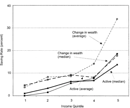
Fig.1.—Median and average saving rates: active saving and change in wealth, PSID, 1984–89. Estimates of the median saving rate are taken from table 3. Average saving rates were calculated by dividing the average level of saving for the quintile by the average level of income; to improve statistical power, the full sample (ages 30–59) was used for the calculation.
picture formed by table 3. Figure 1 shows average saving rates and median saving rates (from table 3) by income quintile for both the change-in-wealth measure of saving and active saving. As in table 2, average saving rates are defined to be average saving for each quintile divided by average five-year income. Although the mean saving rates are somewhat higher than the medians, the patterns are generally sim-ilar except in the top quintile, where the mean change-in-wealth saving rate jumps to 34 percent of income.
B. Saving Rates and Permanent Income
We now turn to the relationship between saving rates and permanent income, using the two-stage procedure described earlier. We first focus on consumption as an instrument. Recall that transitory consumption will bias the estimated slope toward a negative number in all three data sets, as will measurement error in the case of the CEX.
Median Instrumental Variable Regressions of Saving Rate on Income Using Consumption as an Instrument
CEX SCF PSID
Y⫺C DWealth DWealth DWealth⫹Pension Active
Nonauto Consumption (1) Vehicles (2) Food Consumption (3) Weighted Consumption (4) Weighted Consumption (5) Weighted Consumption (6)
Quintile 1 .211
(.010) .028 (.030) .000 (.005) .000 (.004) .077 (.010) .011 (.006)
Quintile 2 .288*
(.008) .140* (.044) .021* (.008) .029* (.008) .124* (.011) .045* (.008)
Quintile 3 .278
(.008) .134 (.039) .033 (.010) .044 (.010) .159* (.013) .053 (.007)
Quintile 4 .283
(.007) .173 (.027) .057* (.010) .078* (.013) .191* (.016) .076* (.008)
Quintile 5 .246
(.007) .286* (.049) .139* (.018) .260* (.032) .344* (.027) .121* (.013)
Top 5% NA .505
(.113)
NA NA NA NA
Top 1% NA .356
(.158)
NA NA NA NA
Ages 30–39 .007
(.007) ⫺ .051 (.029) .005 (.007) .000 (.005) ⫺ .012 (.011) ⫺ .003 (.006)
Ages 50–59 ⫺.001
(.009) ⫺ .016 (.034) .006 (.008) .002 (.007) .042 (.018) ⫺ .011 (.007) Pseudo 2
R .003 .031 .013 .034 .040 .022
Sample size 13,054 728 2,793 2,793 2,793 2,793
Coefficient on income/104 ⫺.003
(.002) .040 (.026) .022 (.003) .035 (.004) .041 (.004) .018 (.002)
Note.—For each column, the top heading indicates the data set used, the second heading indicates the saving measure used, and the third heading indicates the instrument used. Bootstrapped standard errors are shown in parentheses. The SCF and PSID quintiles are weighted; all regressions are unweighted.
median saving rate rises from the predicted first to second quintile but then remains fairly flat. One interpretation is that the results favor the Friedman proportionality hypothesis, but a more likely explanation is that the negative bias associated with transitory consumption and con-sumption measurement error is approximately offset by a positive cor-relation between saving rates and permanent income.
We next consider data from the SCF and PSID, where saving is derived from the change in wealth and is thus likely uncorrelated with sumption measurement error. The SCF does not contain direct con-sumption flow measures, but it does include the reported value of owned vehicles. As shown in column 2, the results when the average of 1983 and 1989 vehicle values is used as an instrument are surprisingly similar to those in table 3, with saving rates rising from 3 percent in the lowest quintile to 29 percent in the top quintile. Saving rates in the top 5 percent are even higher. The estimated linear impact of income on saving rates is roughly four percentage points per $10,000 in income but is not significant at the 5 percent level.
Column 3 of table 4 shows that when PSID food consumption is used as an instrument, the estimated change-in-wealth saving rate rises con-sistently with income.30Indeed, the step-up in the saving rate is signif-icant for every quintile but the third. Columns 4–6 of table 4 use a more comprehensive measure of consumption from the PSID: a weighted average of food at home, food away from home, rental payments, and imputed housing flows, with weights derived from the CEX (Hamermesh 1984; Skinner 1987).31
The estimated gradients of the saving rate with respect to income are similar to (and in some cases slightly larger than) those in table 3.32
Our next approach instruments current income with lagged and fu-ture earnings. For the CEX, we have no data on lagged or fufu-ture earn-ings. For the SCF, we redefine current income (for the purposes of putting households into quintiles) as 1988 income and instrument with 1982 income. Column 1 of table 5 shows that this procedure yields a strong relationship between predicted income and saving rates. Only
30In the first stage, we predict average current disposable income (1984–88) using food
consumption for each year from 1984 to 1987. (The food questions were temporarily suspended in 1988, so that we have no consumption measures for that year.) See Zeldes (1989) for further details on the construction of the food consumption variable.
31More specifically, we calculate the measure for each year from 1984 to 1987, using
weights from Bernheim, Skinner, and Weinberg (2001), so that
weighted
C p1.930(food at home)⫹2.928(food away from home)
⫹1.828(rental payments if renter)⫹.1374(value of house if home owner).
32To save space, we do not report active plus pension and Social Security saving estimates
Median Instrumental Variable Regressions of Saving Rate on Income using Lagged and/or Future Earnings as Instruments
SCF PSID
Lagged Income Lagged Earnings Future Earnings
DWealth
(1)
DWealth
(2)
DWealth⫹
Pension (3) Active (4) DWealth (5)
DWealth⫹
Pension (6)
Active (7)
Quintile 1 .022
(.025) .000 (.004) .065 (.010) .003 (.005) .000 (.003) .063 (.008) .003 (.005)
Quintile 2 .094*
(.027) .024* (.012) .136* (.019) .024* (.009) .025* (.008) .140* (.013) .028* (.009)
Quintile 3 .106
(.036) .059 (.019) .174 (.020) .052* (.011) .057* (.010) .170* (.011) .064* (.008)
Quintile 4 .167
(.028) .081 (.019) .195 (.019) .073 (.013) .072 (.014) .201* (.015) .062 (.009)
Quintile 5 .246
(.035) .115 (.035) .239 (.030) .080 (.016) .170* (.017) .289* (.020) .119* (.010)
Ages 30–39 ⫺.057
(.026) .000 (.008) ⫺ .012 (.016) .006 (.009) .000 (.004) ⫺ .020 (.010) ⫺ .001 (.006)
Ages 50–59 ⫺.016
(.027) .001 (.007) .029 (.018) ⫺.003 (.006) .000 (.004) .010 (.015) ⫺.003 (.006) Pseudo 2
R .041 .013 .022 .017 .025 .041 .030
Sample size 728 1,359 1,359 1,359 2,471 2,471 2,471
Coefficient on income/104 .020
(.005) .014 (.002) .022 (.003) .011 (.002) .026 (.002) .031 (.003) .017 (.002)
Note.—For each column, the top heading indicates the data set used, the second heading indicates the saving measure used, and the third heading indicates the instrument used. Bootstrapped standard errors are shown in parentheses. The SCF and PSID quintiles are weighted; all regressions are unweighted. The SCF results use 1988 income as current income and 1982 income as lagged income. The PSID results use 1974–78 for lagged earnings and 1989–91 for future earnings. The SCF coefficients for the top 5 percent and top 1 percent are .397 (.115) and .455 (.088), respectively.
TABLE 6
Median Regressions of Saving Rate on Education
CEX SCF PSID
Y⫺C
(1) DWealth (2) DWealth (3) DWealth⫹ Pension (4) Active (5) No high school diploma .155
(.009) .057 (.043) .000 (.003) .090 (.009) .020 (.006) High school diploma .284*
(.006) .131 (.031) .039* (.006) .148* (.009) .052* (.007) College degree⫹ .342*
(.007) .323* (.027) .123* (.015) .236* (.014) .102* (.010)
Ages 30–39 ⫺.004
(.007) ⫺.063 (.033) .002 (.005) ⫺.021 (.009) ⫺.006 (.007)
Ages 50–59 .017
(.009) .021 (.046) .008 (.007) .033 (.013) ⫺.017 (.008)
PseudoR2 .017 .025 .014 .020 .014
Sample size 13,054 728 2,840 2,840 2,840
Coefficient on income/104 .060
(.003) .009 (.002) .028 (.003) .033 (.003) .021 (.002)
Note.—For each column, the top heading indicates the data set used and the second heading indicates the saving measure used. Bootstrapped standard errors are shown in parentheses. The regressions are unweighted. Definitions of income: CEX: current income; SCF: average of 1982, 1988 income; PSID: average of 1984–88 income.
* The coefficient is significantly greater than that for the next lower education, on the basis of a one-sided 5 percent test.
one of the differences between quintile estimates is statistically signifi-cant, but the estimate from the linear equation (a two-percentage-point increase for each $10,000 in predicted income) is highly significant.
For the PSID, we use as instruments labor earnings of the head and wife (combined) for each year from 1974 to 1978—10 years before the period over which saving is measured.33
Columns 2, 3, and 4 of table 5 show the results of this approach for the three PSID saving measures. In all cases, saving rates rise with predicted permanent income. The magnitudes of the differences are in fact quite close to those from the uninstrumented results in table 3, suggesting that the simple five-year average of current income eliminates much of the effects of transitory income. Columns 5–7 of table 5 show that when future earnings (1989– 91) are used as instruments, we again see saving rates increasing with predicted income. This is true whether one looks at the quintile coef-ficients (ranging, for the change-in-wealth plus pension saving measure, from 6 percent to 29 percent) or the coefficient from the regression on predicted income.
In table 6, we next turn to education as an instrument—a proxy for permanent income that is generally fixed over the life cycle. For the
33We have earnings information back to 1967, but when we condition on earnings in
more recent years, the earlier earnings added little or no predictive power for income in 1984–88.