Vol 8, No 9 (2019)

(1)

COMPUTATION OF CHEMICAL POTENTIAL AND FERMI-

DIRAC INTEGRALS APPLIED TO STUDY THE TRANSPORT

PHENOMENA OF SEMICONDUCTORS

R. Kobaidze

[a] [b]

_{, E. Khutsishvili}

[a] [b]

**_{*, Z. Chubinishvili}**

[a] [c]

_{, G. Kekelidze}

[d]

_{, N.}

Kekelidze †

Keywords:

Chemical potential, Fermi–Dirac integrals, Gauss–Legendre method

In the given paper, two methods of calculating with high precision accuracy the chemical potential and the integrals of the type called the

Fermi–Dirac of different indexes are presented. Our calculations are conclusive with already existing data. These data are essential not only

in the study of the theory of solids but at the explanation of the experimental results of investigated transport phenomena in solids, namely,

in semiconductors.

* Corresponding Author:

E-Mail: [email protected]

[a] Laboratory of Semiconductor Materials Science, Ferdinand

Tavadze Institute of Materials Science and Metallurgy, Tbilisi,

0186, Georgia

[b] Institute of Materials Research, Ivane Javakhishvili Tbilisi

State University, Tbilisi 0179, Georgia

[c]

Department of Engineering Physics, Georgian Technical

University, Tbilisi, 0175, Georgia

[d]

NPO “International Innovative Technologies”, Tbilisi, 0192,

Georgia

Introduction

The physical laws of systems consisting of a huge number

of particles are of a statistical nature. Statistical distribution

determines the probability of having those or other defining

states parameters of the particles of the system.

1

_{One example}

of systems of the huge number of particles that requires a

statistical approach is the solid state, in particular,

semiconductors. The distribution of electrons over energies,

namely, the Fermi–Dirac distribution, is the most important.

The Boltzmann distribution, which is valid for particles

obeying classical mechanics, is the limiting case of the

Fermi-Dirac distribution. In the state of statistical equilibrium, the

ideal electrons gas in solid state obeys the Fermi–Dirac

statistics.

2,3

_{Different physical phenomena are differently}

sensitive to the type of statistical distribution. When

considering the transport properties in a solid state, we

inevitably collide with integrals of the type called the Fermi–

Dirac integrals.

2,3

_{These are certain integrals often}

encountered not only in the study of the theory of

semiconductors but at the explanation of the experimental

results of investigated transport phenomena in

semiconductors.

In this case, we have to use not only the tables of values of

the Fermi integral but also their approximate formulas.

4

However, the calculation of integrals according to

approximate formulas and tables gives a sufficiently high

value of error, especially for large and small values of the

reduced Fermi level. The error can reach approximately 25%.

Using approximations is inconvenient and inaccurate.

Therefore, the goal of our paper is to find an appropriate

method for calculation of the Fermi–Dirac integrals for

application in the study of semiconductors properties with

high accuracy <<1%. The presented paper allows also

determining a normalization constant, included in the Fermi–

Dirac statistics, - the chemical potential with high reasonable

accuracy.

Methodology

Gauss–Legendre method integrals solution

Functional integral according to Gauss–Legendre method is

presented as the sum of (

n-1

) coefficients:

.

(1)

Let’s say, at searching of integral we foresee only 2

coefficients, then it follows from (1):

(2)

This expression consists of 4 unknown coefficients (

C

0

,

C

1

,

x

0

,

x

1

) and, consequently, we need 4 boundary conditions:

f

=

const

f

=

x

f

=

x

2

3

f

=

x

(3)

The value of integral may be taken at an arbitrary [

a

,

b

]

boundary. In our case, we take [–1,1] interval and const=1.

From (3), boundary conditions follow:

(4)

The solution of (4) equations gives the following values for

C

and

x

coefficients:

0

( )

0 1

( )

1 2

( )

2 3

( ) ...

3 n 1

(

n 1

)

I

≈

C f x

+

C f x

+

C f x

+

C f x

+ +

C

−

f x

−

0

(

0

)

1

( )

1

I

≈

C f x

+

C f x

1

0 0 1 1

1 1

0 0 1 1

1 1

2

0 0 1 1

1 1 3

0 0 1 1

1

1 (

)

( )

2 (

)

( )

0

2 (

)

( )

3 (

)

( )

0 dx C f x

C f x

xdx C f x

C f x

x dx C f x

C f x

x dx C f x

C f x

−

=

+

=

+

=

+

=

+

=

∫

(2)

(5)

Taking into account the value of two coefficients, the

magnitude of integral is:

(6)

Taking into account 4 coefficients, we have to add 4

boundary conditions:

f

=

x

4

_,

_f

₌

_x

5

_,

_f

₌

_x

6

_,

_f

₌

_x

7

_{. At these boundary}

conditions calculated coefficients are:

(7)

These coefficients are needed to be installed into (1) for

calculation of the digital value of integral. If we take into

account

n

coefficients, we will need 2

n

boundary conditions.

In general, our task is to solve integral

in arbitrary boundaries. For calculation of integral, it is

necessary to transfer the boundary [a,b] into [–1,1]. Let’s say,

the value of the new argument is given by:

(8)

and we search the integral value in the form of

because integrals values are equal to each other:

From this it follows new conditions:

Finally, for integral solved with two coefficients we obtain

formula:

.

(9)

The more terms we take into account in the formula (1), the

more accurate value of integral will be. In general, taking into

n

coefficients:

(10)

where ƒ(

x

) is an arbitrary function, which is continuous in

[a,b] interval and

C

i

and

x

i

are coefficients found from

boundary conditions.

The second way to calculate

C

i

and

x

i

coefficients is to solve

Legendre polynomial equitations:

5,6

(11)

(12)

To obtain

C

i

and

x

i

coefficients, first, we have to generate

Legendre polynomials and solve them. We can use

MATLAB-s built-in functions to generate polynomials and

solve them

7

_{(legendrePolynomials_1.m), or we can manually}

generate. Program

(legendrePolynomials_2.m) uses

polynomials properties:

5

,

(13)

These values are uploaded on the repository (roots_2,

weights_2).

7

Method of undefined integrals solution

Let’s say the integral is not given in limited [

a

,

b

] interval,

but in [0,

+∞]

range. We can decompose integral into two

parts:

.

(14)

In the second part of integral, we substitute the variable:

0 0

1 1

1

3

1

3 C

x

C

x

=

= −

=

1

1 (

)

(

)

3

3 I

=

f

−

+

f

0 2

1 3

18

30

18

30

36

18

30

18

30

36

36 C

C

−

+

=

+

−

=

0 2

1 3

525 70 30

35

35 525 70 30

525 70 30

35

35 x

x

+

−

= −

=

−

+

= −

=

( )

b

a

I

=

∫

f x dx

1 2 d

x

= +

a

a x

1

( )

_d _d

I

f x dx

−

=

∫

1

(

)

( )

b

d d

a

I

f x dx

I

f x dx

−

=

_∫

=

_∫

1 2

a

b

a

+

=

−

=

d

2

2 b

a

b

a

x

=

+

−

x

d

2 b

a

dx

=

−

dx

b 1

d d

a 1

( )

2

2 b a

a b

b a

f x dx

f

x dx

−



+

−



=

_

+

_





∫

b n

i i

i 1 a

( )

2

2 b

a

b

a

f x dx

C

f

x

=

−



+

−



=

_

+

_





∑

∫

n

(

i

)

0 P x

=

2 i

i 2

n 1 i

2(1

)

[

( ) ]

x

C

nP

₋

x

−

=

0 1

( )

1 ( )

P x

x

=

2 2

3 3

1 ( )

(3

1)

2

1 ( )

(5

3 )

2 P x

x

P x

x

=

−

=

−

( n 1) n n 1

2

1 ( )

( )

1

1 n

n

P

xP x

P

x

n

+ −

+

=

−

+

1

0 0 1

( )

f x dx

∞ ∞

=

+

∫

1 t

x

=

dx

1

₂

dt

t

= −

1

0 x

t

x

t

=

(3)

Finally, we obtain formula (15) for approximate calculation

of integral:

(15)

We can apply (10) formula to the two parts of this integral

and solve any integral, which is defined in this range. Taking

into account (14) and (15) formulas, we obtain:

(16)

Calculation of integrals by (16) formulas and their

summation give the final meaning of (14) integral.

Integral Fermi and its derivative

The general view of integrals of Fermi is given by the

formula:

(17)

where

ξ

is the chemical potential. Many authors do not take

into account

Γ( +

k

1)

member and introduce integral Fermi

as:

(18)

The formula for Fermi integrals derivative is given by:

(19)

For gamma function, given in (17) formula, it can be

written:

If

n

is a natural number,

It is also known, that

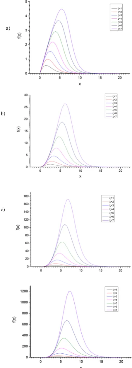
The graphics of integrand function in (18) formula for

different values of

k

and

ξ

are given in Fig.1. It is clear from

Fig.1 that these functions are decomposable and it is possible

to integrate them in certain approximation.

a)

b)

c)

Figure 1

. Dependence of integrand functions of Fermi integrals of

different indexes (

k

) on

x

coefficient (parameter in Gauss–Legendre

decomposition) for different values of chemical potential (

ξ

)

according (18) formula.a)

k

= 1; b)

k

= 2; c)

k

=

3; d)

k

=

4

1 1

2

0 0 0

1

1 ( )

( )

(

)

f x dx

f

dt

t

∞

=

+

∫

1 n

i i

i 1 0

( )

0.5 (0.5 0.5 )

f x dx

C

f

x

=

∑

+

∫

1 n

i

i 0 i i

0

1

1 (

)

0.5 (

)

0.5 0.5

f

dt

C

f

t

=

x

=

+

∑

∫

( )

0

1 (

1)

1

k

k x

x dx

F

k

e

ξ

) =

∞ ₋

Γ( +

∫

+

( ) 0

(

1

k

k x

x dx

F

e

ξ

) =

∞ ₋

+

∫

( )

( 1)

(

k k

dF

F

d

ξ

−

)

=

)

( )

n

(

n

1)!

Γ

=

−

(

n

1)

n

( )

n

Γ + = Γ

1 ( )

2 π

Γ

=

3 ( )

2

2 π

(4)

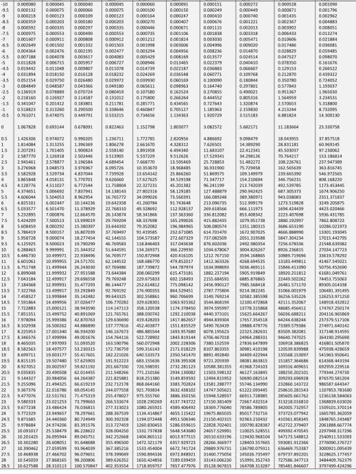
Table 1.

Fermi integrals calculated using Gauss–Legendre numerical method for different

k

and

ξ values.

ξ F(-0.5)(ξ) F(0)(ξ) F(0.5)(ξ) F(1)(ξ) F(1.5)(ξ) F(2)(ξ) F(2.5)(ξ) F(3)(ξ) F(3.5)(ξ) F(4)(ξ)

(5)

29 29.5 30

10.723418 10.834220 10.954374

28.828660 29.431761 30.087872

103.379363 106.663945 110.248115

417.578079 435.476104 455.062998

1801.457447 1899.035693 2006.114497

8105.944774 8638.191699 9223.788410

37565.730293 40470.262904 43673.935454

177957.836926 193815.317953 211348.075056

857572.092172 944184.493311 1040169.670945

4189989.132597 4663258.212882 5188924.669727

Finally, the Fermi integrals values have been calculated by

the Gauss–Legendre method, where

C

i

and

x

i

coefficients

have been found from (11) and (12) formulas. The Program

has been written in Matlab programming language

(Fermi_integral_calculator_1.m) and it uses 100 points of

Gauss–Legendre coefficients.

7

_{The values of calculated Fermi}

integrals for different parameters

k

and

ξ

are given in Table 1.

Simson’s integral calculation method

Another way to calculate integrals of function

f

(

x

), which

are defined in [

a

,

b

] range, is Simson’s

integration method, the

general formula of which is given in (20):

7

(20)

Results for Simson’s rule are in good agreement with the

Gauss–Legendre method.

Error estimation

Finally, we show the advantages of the method presented in

the article by calculating the error of implemented

calculations.

Gauss–Legendre method error estimation has been done by

using (21) formula:

(21)

where

(22)

and

a

≤ ≤

θ

b

.

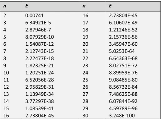
The values of

E

parameter estimated by (22) formula are

given for different

n

in Table 2.

Table 2.

Values of

E

according to (22) formula for different

n

E

n

E

2

3

4

5

6

7

8

9

10

11

12

13

14

15

16 0.00741

6.34921E-5

2.87946E-7

8.07929E-10

1.54087E-12

2.12743E-15

2.22477E-18

1.82325E-21

1.20251E-24

6.52056E-28

2.95829E-31

1.13949E-34

3.77297E-38

1.08539E-41

2.73804E-45

16

17

18

19

20

21

22

23

24

25

26

27

28

29

30 2.73804E-45

6.10607E-49

1.21246E-52

2.15736E-56

3.45947E-60

5.0253E-64

6.64363E-68

8.02751E-72

8.89959E-76

9.08485E-80

8.56732E-84

7.48625E-88

6.07844E-92

4.59789E-96

3.248E-100

It is clear that the increase of

n

-value decreases the value of

E

and error goes to nearly zero.

Conclusion

The chemical potential and Fermi–Dirac integrals are

essential for a basic understanding of semiconductors

properties. In this paper, there have been calculated Fermi–

Dirac integrals by two different ways – Gauss–Legendre and

Simson’s methods. Both methods are in good agreement with

each other. Our data let reduce the error of calculation of

Fermi–Dirac integrals up to <<1%.

Acknowledgment

Paper was presented at the 5th International Conference

"Nanotechnologies," November 19–22, 2018, Tbilisi, Georgia

(Nano–2018).

References

1

_{Lifshitz, E. M., and Pitaevski}

ǐ

_{, L. P.,}

_{Statistical physics}

_{/ Part 2,}

Theory of the condensed state

, Oxford; New Yor : Pergamon

Press,

1980

.

2

_{Blatt, F. J.,}

_{Theory of Mobility of Electrons in Solids}

_{, Academic}

Press Inc., New York,

1957

.

3

_{Anselm, A. I.,}

_{Introduction to the Theory of Semiconductors}

_{, Nauka,}

Moscow,

1978

.

4

_{Fistul, V. I.,}

_{Heavily doped semiconductors}

_{, Phys.-Math. Lit. Press,}

Moscow,

1967

.

5

_{Davis P. and Rabinowitz, P., Abscissas and Weights for Gaussian}

Quadratures of High Order,

J. Res. Natl. Bureau Standards

,

1956

,

56(1),

35-37.

https://nvlpubs.nist.gov/nistpubs/jres/56/jresv56n1p35_A1b.pd

f

b

a

x

n

−

∆ =

b

a

( )

(First Last 4(sum of odds) 2(sum of evens))

3 x

f x dx

=

∆

+

∫

(2n 1) 4

3

2 ( !)

(2

1)((2 )!)

n

E

n

+

=

+

(2n )

Error

=

Ef

( )

θ

b

1 3

a

5 2n 1 2

4 6 2n

( )

( ( )

( )

4( ( )

( ) ...

3 ( )

(

))

2( (

) ...

(

)

(

) ... (

)))

x

f x dx

f a

f b

f x

+

∆

=

+

(6)

6

_{http://keisan.casio.com/exec/system/1280883022.}

7

_{https://github.com/scienceman001/Fermi-integrals.}

8

_{https://www.intmath.com/integration/6-simpsons-rule.php.}