Proceedings of the
4th International Workshop on
Multi-Paradigm Modeling
(MPM 2010)
A Visual Notation for Declarative Behaviour Specification
Thomas Kühne
10 pages
Guest Editors: Vasco Amaral, Hans Vangheluwe, Cécile Hardebolle, Lazlo Lengyel Managing Editors: Tiziana Margaria, Julia Padberg, Gabriele Taentzer
A Visual Notation for Declarative Behaviour Specification
Thomas Kühne
Victoria University of Wellington
Abstract: Logical programming has many merits that should appeal to modellers. It enables declarative specifications that are free from implementation details and even (mostly) abstracts away from control flow specification. However, the textual syntax of, for example PROLOG, most likely represents a barrier to the adoption of such languages in the modelling community. The visual notation presented in this paper aims to facilitate the understanding of behaviour specifications based on logic programming. I anticipate that the dataflow-like nature of the resulting diagrams will appeal to modellers. I believe the visual notation to be an improvement over the traditional textual syntax for the purpose of specifying PROLOG programs as such, but the ultimate hope is to have found a vehicle to make declarative logic programming a commonplace activity in multi-paradigm modelling.
Keywords:behaviour modelling, declarative specification, visual syntax
1
Introduction
Modelling the structure of a subject is well supported by existing languages. For instance, UML class diagrams [BRJ98] have successfully been used to model the structure of problem domains and software systems. In general, however, modelling the subject’s behaviour is much more challenging. Typically, the set of all possible behaviour traces is much more complex than the structure that supports it. As with structural modelling, in behaviour modelling a finite, static description has to be used, however, in this case to capture dynamic behaviour with a multitude of variations, case distinctions, etc. There is an intrinsic disconnect between the static description of behaviour and the latter’s temporal character that supports a potentially infinite unfolding of branches.
By restricting the behaviour to be described to simple reactive behaviour, as exhibited by many small embedded systems, it becomes possible to use notations such as UML state diagrams to in-tuitively and completely capture their behaviour [MB02]. However, when faced with describing more complex behaviour, it seems that one of the three following approaches has to be adopted:
1. Visual notations, such as activity diagrams and interaction diagrams, are regarded as con-straining potential behaviour, but no attempt is made to completely specify the behaviour.
2. Visual notations, such as state diagrams and the above, are extended with action languages. The visual notation thus provides the structure into which conventional behaviour specifi-cation fragments are embedded.
It is outside the scope of this paper to provide empirical evidence for the following assumptions but we will nevertheless assume them to be true in the context of this paper:
• It is desirable to avoid unnecessary media changes. If many properties of the system are described using a visual notation, one should not add textual notations to the mix unless there is a good reason for doing so.
• Some textual descriptions can benefit from being transcribed into a visual notation in order to acknowledge their graph-like (as opposed to tree-like) structure.
In multi-paradigm modelling typically a large variety of different notations will be used and I believe the modeller’s experience will be improved if they can use visual models most of the time, in particular if the visual form is more appropriate to do justice to graph-like descriptions.
In this paper, I propose to use a declarative formalism for modelling behaviour (Section 2) and present a visual notation for it (Section 3), arguing that the visual form bears a number of advantages. I then discuss related work (Section 4) and conclude with a final discussion (Section 5).
2
Declarative Behaviour Specification
The intention of modelling is to focus on the “What?” not on the “How?”. This is why declara-tive formalisms lend themselves to be used in modelling. Logic programming languages could be regarded as quintessential behaviour modelling languages since they attempt to describe the be-haviour logic only, leaving control aspects to inference engines [Kow79]. Execution is achieved by logical inference and in principle the inference engine could use one of many ways to execute the specified logic.
A well-known logic programming language is PROLOG[CR92]. It is one of the most declar-ative programming languages in existence because
• unification is directionless. In general, any parameter of a PROLOG predicate may be used as an input parameter, or output parameter, or precondition, depending on how the predicate is used.
• PROLOGdefines relations rather than functions. As a result, one relation definition often substitutes a number of function definitions.
• control flow is implicit rather than explicitly specified. A PROLOGprogram specifies facts and rules but no explicit control flow1.
All the above make PROLOGa formalism that should be very useful in modelling and indeed it has already been used for the specification of transformations [CH03].
Arguments against PROLOGinclude
1. it is difficult to structure large PROLOGprograms.
2. the textual notation is rather dense and will likely meet reservations from modellers used to visual notations.
3. it is easier to write PROLOG programs than to read them. The fact that only the bare essentials are expressed and that a PROLOGpredicate can often be used in a multitude of ways, can make it hard to understand PROLOGprograms.
There is hope that by using other models as structuring aids, it will be possible to address the first of the above issues. In this paper, however, I propose a visual syntax for PROLOG(the abstract syntax and semantics from PROLOG are retained) that I believe to somewhat alleviate the last two of the above issues.
3
Visual Notation
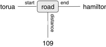
A typical problem of reading and writing PROLOG programs is that one is not sure about the meaning and role of parameters. For instance, inListing 1it is not clear whether Peter is Paul’s parent or vice versa. Likewise, the road description could first specify the destination and then the starting point or vice versa. The number at the third position could be among other things a road ID, the label of a motorway, or a distance specification.
parent ( peter , paul ).
road( rotorua , hamilton , 109).
Listing 1: PROLOGFact Definitions
This problem can be addressed through comments or using descriptive formal parameter names for other clauses that use the same functor, but in either case the information is at a different location and potentially there are no clauses which could list descriptive formal parameter names.
road hamilton
dis
tanc
e
rotorua
109
end start
Figure 1: Visual Fact Notations
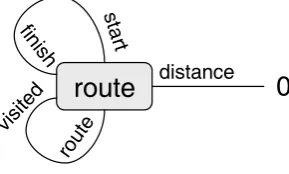
route ( Finish , Finish , Visited , Visited , 0).
route ( Start , Finish , Visited , Route, Distance ) :− road( Start , End, Length ),
not(member(End, Visited )),
route (End, Finish , [ Start | Visited ], Route, AccumulatedDistance), Distance is Length + AccumulatedDistance.
Listing 2: PROLOGRoute Clauses
Listing 2shows the definition of a PROLOGpredicate that will compute all possible routes be-tween two cities including the respective distances.
Note that it is next to impossible to understand the meaning of the first clause without consult-ing the second clause in order to gain an understandconsult-ing of the parameter roles. The first clause states that if the start and the finish positions are identical then the route is identical to list of previously visited cities and the distance between the start and finish locations is zero.
ConsiderFigure 2and note how much easier it is to attain the same understanding of the first clause without consulting any other location of the specification.
route
start fin
ish
0
distance
rout
e visite
d
Figure 2: First Route Clause
Lines connecting parameters with each other state that these parameters have to have the same value. PROLOGunification applies so no statement is made whether a start value is transferred to a finish value or vice versa, or whether two values are compared.
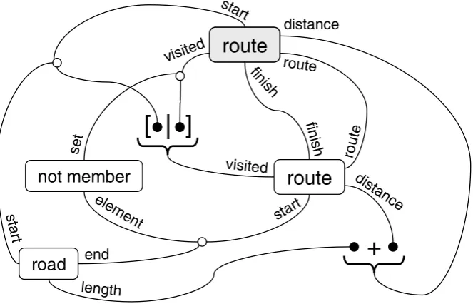
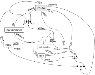
The second route clause ofListing 2is more interesting as it involves other predicates. Fig-ure 3shows the same clause in my proposed visual notation. Several observations can be made regardingFigure 3:
finis h
road
start
distance
route
visited
route
route
end
length
start
not member
+
set
elem
ent start
fin ish
[ | ]
[ | ]
visited ro
ute
distance
route
Figure 3: Second Route Clause
• the keyword parameters help to understand the significance of a value for a predicate used as a premise. For instance, it is possible to figure out that the “[Start | Visited]” value at the third position of the “route” premise is meant to be the updated list of visited locations but this requires looking up the formal parameter name of the clause definition. In comparison, the “visited” role of the “route” premise in the visual notation makes it explicit in what way the value is going to be used.
• variable names can appear in more than two places which results in more than two roles being connected by the same line. I currently use little circles as explicit junction points for such n-ary connectors. It is possible to annotate these connectors or lines in order to communicate the role of a value in the context of a clause definition. For instance, one could add an “accumulated distance” annotation to the line that connects “route” with the second operand of the addition operator.
• the graph shown inFigure 3offers a direct visual insight into the topology of the clause definition. Akin to a dataflow diagram it becomes readily apparent how values are used to form new aggregates or feed into further computations. Consider the connection between the “road” and “route” premises. It becomes evident that the end point of the road used in the route becomes the start point of the sub-route that needs to be computed. The same can be inferred from the textual version in Listing 2 but it requires to find locate two occurrences of the “End” variable and one has to look for the connection while it is has been turned into explicit geometry inFigure 3.
is not encoded by multiple variable occurrences using the same name but becomes explicitly apparent by using visual connectors. The fundamental purpose of using a variable in two posi-tions (e.g., “End” in the “road” and “route” premisses) is to connect the two positions. Any arbitrary variable name like “X” would have worked as well. The (potentially n-ary) line in the visual form does just this; it connects positions that need to be connected. If the relevance of the connections is not clear from all the role names involved, one can annotate the line with a label, such as “intermediate location”.
3.1 Further Applications
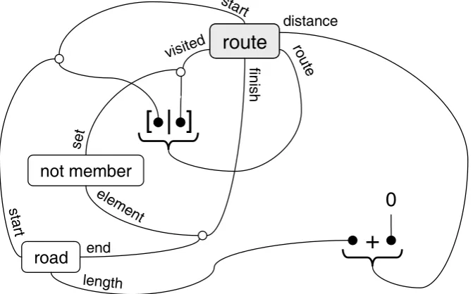
The graphs created using the visual notation lend themselves to unfolding of premisses. For instance, there are two possibilities in which the “route” premise ofFigure 3may be unfolded. Either the clause shown inFigure 2or that inFigure 3applies.
Figure 4 shows the resulting structure if the first clause is inserted within the second. This corresponds to the situation where the final location of a route has been found. It is very easy to manually insert the structure ofFigure 2into that of Figure 3(in this case this mainly leads to connection shortcuts) but ideally there should be tool support for this.
road
start
distance ro
ute visited
route
route
end
length
start
not member
+
set
elem ent
finish
[ | ]
[ | ]
0
Figure 4: Unfolding Using the First Route Clause
Figure 5shows the insertion of the second clause into itself. This particular unfolding is useful to illustrate the recursive nature of the second clause. One can clearly see how the “visited” list is built up by successive additions of elements to the head of the list.
Unfolding operations such as the above are useful to check whether special cases are handled correctly and/or whether the clauses cooperate with each other as intended. The unfolded graphs will reveal unexpected structures in case the clause definitions are erroneous.
road
sta rt
distance
route
visited routeroute
end
length
start
not member
+
set
elem ent
fin ish
[ | ]
[ | ]
visited
finis h
road sta
rt end
length
not member
+ set
element
start
[ | ]
visited
rout e
distance
route
Figure 5: Unfolding Using the Second Route Clause
the “visited” locations and hence will not appear as part of the “route” result. After having looked atFigure 5, a developer will also know that the “visited” locations, and hence the locations in the “route” result are in reverse order. Both these facts are not as apparent from the textual clause definitions inListing 2. The reverse ordering of the locations is caused by the use of an accumulator technique which makes the “route” predicate more efficient. This “route” predicate version was deliberately chosen over a more straightforward definition in order to demonstrate the efficacy of the visual notation in making the reverse ordering apparent.
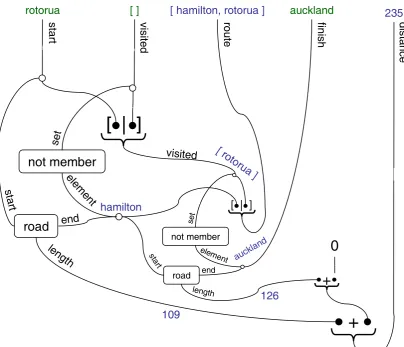
Another use for the visual notation is shown inFigure 6. Here actual values have been provided for “start”, “visited”, and “finish” and the graph shows how these values yield the “route” and “distance” results. Again, a simple unfolding of premises using the appropriate clause definitions is all that is required to produce the graph inFigure 6. Note how actual values flowing between premises are shown as annotations, in this example “hamilton”, “auckland” and the distance values. Such usage scenario graphs could prove to be useful for debugging purposes or helping to understand how a predicate works prior to using it.
4
Related Work
pro-visite d
road
sta rt end length rotoruanot member
+
set elem ent[ | ]
[ | ]
visited road start end length not member+
set element [ | ] [ ] start distanc
e
235
ro
ut
e
[ hamilton, rotorua ] auckland
fin ish hamilton auckla nd 109 126
0
[ rotorua ]
Figure 6: Actual Usage Scenario
vides a better understanding of the topology of an execution graph. Currently, my visualisation approach does not aim at indicating potential future continuations of execution or depicting past computations and is therefore not as suited as AND/OR trees for such purposes.
SLDNF-DRAWis visualisation system used to support the teaching of PROLOG[Gav07]. As with AND/OR trees, lines between predicates are motivated by the call graph, not by corefer-enced variables. As a result, the system is successful in showing PROLOGexecution including the extra-logical “cut” operator, but does not provide insights into the dataflow between premises in clause definitions.
LOGICHART was developed to visualise the execution flow of PROLOG programs [AF07]. Similar to AND/OR trees, no attempt is made to visualise the connections between predicate argument positions. These connections have to be inferred by matching variable names. It is possible that the LOGICHARTwork on obtaining optimal layouts [ATIY99] is transferable to the visual notation presented here.
The respective visualisation also uses lines to show variable coreference but visual embedding is used to depict logical inclusion. As a result, the program visualisation seems to yield far less intuitive diagrams compared to the approach presented in this paper.
Puigsegur et al. also use set inclusion relationships in order to derive a visual layout based on embedding [PAR96,PAR98]. While the resulting diagrams may be regarded as intuitive for relations which can be thought of having a set and membership underpinning, the further the stretch to that underpinning, the less intuitive the diagrams appear. The diagrams are not very self-explanatory, in particular because connectors do not use role names. I am of the opinion that the approach by Puigsegur et al. overlays a set metaphor on top of the generic relations paradigm that, overall, just adds a complication rather than being helpful. Further research is required to evaluate whether the notation proposed in this paper is actually easier to use in practice.
VPL aims to use visualisations to emphasise the relational nature of logic programming. It supports program composition and editing in both textual and graphical representations [LR91]. VPL also presents predicates as boxes but replaces variable names with graphical patterns. The task to infer coreferenced variables is therefore turned into the arguably even harder task of matching patterns. The visual notation captures logical conjunction and disjunction. The ap-proach presented in this paper always assumes logical conjunction within one diagram and re-quires the use of multiple diagrams for including disjunction. It remains to be seen which ap-proach is more advantageous in practice.
5
Conclusion
In this paper I argued that logical programming has many merits that should appeal to modellers. I briefly discussed PROLOGas a well-known example for a declarative language that enables the specification of many functions through the definition of comparatively fewer relations.
I speculated that the dense textual syntax and the resulting “easier to write than to read ”-character of such languages may have been a barrier for adopting such approaches in modelling. The visual notation presented in this paper is hoped to facilitate the understanding of PROLOG programs by PROLOG programmers, but the fact that role names as known from UML class diagrams are used and that the resulting diagrams resemble dataflow diagrams should appeal to modellers in particular.
Part of the effectiveness of the visual notation derives from the fact that coreferencing is made visually explicit. Instead of requiring the reader to infer the coreferencing through matching vari-able names, the visual notation shows how predicate argument positions are connected through n-ary connectors. One could argue that PROLOGclause definitions have an inherent graph struc-ture and that the visual notation is the more natural one to do justice to this property.
Note that it is trivial to translate any of the diagrams presented in this paper to executable PROLOG programs. A modeller can therefore obtain an executable behaviour specification by simply drawing diagrams in the spirit as presented here.
Bibliography
[AF07] Y. Adachi, Y. Furusawa. Logichart: A Prolog Program Diagram and its Layout. ECE-ASST7, 2007.
[ATIY99] Y. Adachi, K. Tsuchida, T. Imaki, T. Yaku. Logichart - Intelligible Program Diagram for Prolog and its Processing System.Electr. Notes Theor. Comput. Sci.30(4), 1999.
[BRJ98] G. Booch, J. Rumbaugh, I. Jacobson.The Unified Modeling Language User Guide. Addison-Wesley, 1998.
[CH03] K. Czarnecki, S. Helsen. Classification of Model Transformation Approaches. In
OOPSLA’03 Workshop on the Generative Techniques in the Context Of Model-Driven Architecture. 2003.
[CR92] A. Colmerauer, P. Roussel. The birth of Prolog. InSecond ACM SIGPLAN conference on History of programming languages. Pp. 37–52. 1992.
[Gav07] M. Gavanelli. SLDNF-Draw: a visualisation tool of prolog operational semantics. CEUR workshop proceedings, ISSN 1613-0073, 2007.
[Kow79] R. Kowalski. Algorithm = Logic + Control. Communications of the ACM 22:424– 436, July 1979.
[LR91] D. Ladret, M. Rueher. VLP: a visual logic programming language.J. Vis. Lang. Com-put.2(2):163–188, 1991.
doi:http://dx.doi.org/10.1016/S1045-926X(05)80028-X
[MB02] S. J. Mellor, M. J. Balcer.Executable UML: A Foundation for Model-Driven Archi-tecture. Addison-Wesley, 2002.
[PAR96] J. Puigsegur, J. Agusti, D. Robertson. A Visual Logic Programming Language.Visual Languages, IEEE Symposium on0:214, 1996.
doi:http://doi.ieeecomputersociety.org/10.1109/VL.1996.545290
[PAR98] J. Puigsegur, J. Agusti, D. Robertson. A Visual Syntax for Logic and Logic Pro-gramming.JOURNAL OF VISUAL LANGUAGES AND COMPUTING9(4):399–428, 1998.