including odd-
A
and odd-odd nuclei, with the Skyrme finite-amplitude method
T. Shafer∗ and J. Engel†Department of Physics and Astronomy, CB 3255, University of North Carolina, Chapel Hill, NC 27599-3255
C. Fr¨ohlich and G. C. McLaughlin
Department of Physics, NC State University, Box 8202, Raleigh, NC 27695
M. Mumpower
Department of Physics, University of Notre Dame, Notre Dame, IN 46556 and Theory Division, Los Alamos National Laboratory, Los Alamos, NM 87544
R. Surman
Department of Physics, University of Notre Dame, Notre Dame, IN 46556 (Dated: May 14, 2018)
After identifying the nuclei in theA'80 andA'160 regions for whichβ-decay rates have the greatest effect on weak and mainr-process abundance patterns, we apply the finite-amplitude method (FAM) with Skyrme energy-density functionals (EDFs) to calculateβ-decay half-lives of those nuclei in the quasiparticle random-phase approximation (QRPA). We use the equal filling approximation to extend our implementation of the charge-changing FAM, which incorporates pairing correlations and allows axially symmetric deformation, to odd-A and odd-odd nuclei. Within this framework we find differences of up to a factor of seven between our calculatedβ-decay half-lives and those of previous efforts. Repeated calculations withA'160 nuclei and multiple EDFs show a spread of two to four inβ-decay half-lives, with differences in calculatedQvalues playing an important role. We investigate the implications of these results forr-process simulations.
I. INTRODUCTION
The solar abundances of nuclei heavier than iron, on the neutron-rich side of stability, have traditionally been attributed to rapid neutron-capture, or r-process, nu-cleosynthesis [1]. The three largest abundance peaks in the solar pattern, at A ∼ 80, 130, and 195, are associ-ated with the closed neutron shells atN = 50, 82, and 126, suggesting that astrophysical conditions of increasing neutron-richness are responsible for each. A smaller fourth abundance peak in the rare-earth elements (A∼160) is also formed in neutron-rich environments. Observational data from meteorites and metal-poor halo stars confirm the separate origins for 70 . A . 120 (“weak”) and A >120 (“main”)r-process nuclei and provide hints of the nature of ther-process astrophysical site, though the exact site (or sites) has not yet been definitively pinned down [2].
In principle ther-process sites can be identified by com-paring simulations of prospective astrophysical environ-ments with observational data from the solar system and other stars (see, e.g., Ref. [3]). The precision ofr-process abundance predictions, however, is limited by our incom-plete knowledge of properties—such as masses, reaction rates, and decay lifetimes—of nuclei on the neutron-rich side of stability [4]. It is particularly important that we
better determine decay lifetimes, sincer-process nuclei are built up via a sequence of captures andβ decays. Thus, β-decay lifetimes determine the relative abundances of the nuclei along ther-process path [1,2,5] and the over-all timescale for neutron capture [6, 7]. At late times, as nuclei move back from the r-process path towards stability and the last remaining neutrons are captured, the lifetimes determine the shape of the final abundance pattern [5,8]. Finally, for a weakr processβ-decay rates control the amount of material that remains trapped in theA∼80 peak and the amount that moves to higher mass numbers [9], i.e. they determine where the weakr
process terminates. For all these reasons, an accurate picture of theβ decay of neutron-rich nuclei is crucial for the accuracy ofr-process simulations.
Although manyβ-decay lifetimes have been measured (see, e.g., Refs. [9–13]), most of the nuclei populated dur-ing ther process remain out of reach. Simulations must therefore rely on calculated lifetimes. The most widely-used sets of theoretical rates are from gross theory [14–16] and from an application of the quasiparticle random-phase approximation (QRPA) within a macroscopic-microscopic framework [6, 17] that employs gross theory for first-forbidden transitions. Here we use a fully microscopic Skyrme QRPA, implemented through the proton-neutron finite-amplitude method (pnFAM) [18] and extended to treat odd-Aand odd-odd nuclei (hereafter “odd” nuclei) in the equal-filling approximation (EFA) [19]. We can now use arbitrary Skyrme energy-density functionals (EDFs) to self-consistently computeβ-decay rates of both even-even and odd axially-symmetric nuclei, including
butions of both allowed (Jπ = 1+) and first-forbidden (Jπ= 0−, 1−, or 2−) transitions.
We evaluate lifetimes for key r-process nuclei in two highly populated regions of the abundance pattern: the large maximum at A ∼ 80 and the smaller rare earth peak at A ∼ 160. In a main r-process, the rare earth peak forms in a different way than do the large peaks at A∼130 and 195, both of which originate from long-lived “waiting points” near closed neutron shells atN= 82 and 126. The rare earth peak, by contrast, forms during the late stages of ther process, as β decay, neutron capture, and photo-dissociation all compete with one another and ther-process path moves toward stability [20,21]. The A∼160 abundance peak is thus useful for studying the mainr-process environment [22,23]. TheA∼80 region is not so clearly related to the mainr process. In fact, nuclei with 70.A.120 can be created in a variety of nucleosynthetic processes, ranging from the neutron-rich weakr process to the proton-richνpprocess [24–26] (see also Refs. [27,28]). Untangling the various contributions to these elements requires rigorous abundance pattern predictions, which in turn require a better knowledge of still unmeasuredβ-decay half-lives.
In this paper, we aim to study and improver-process abundance predictions for both weakr-process nuclei and the rare-earth elements by identifying and recalculating key β-decay rates. We begin in Sec. II by reviewing the pnFAM and then discussing our extension to odd nuclei. In Sec.III, guided byr-process sensitivity studies, we calculateβ-decay rates separately for the important isotopes in the two mass regions (after optimizing the Skyrme EDF separately for each region). We also examine the effect onβ-decay half-lives of varying the Skyrme EDF in rare-earth nuclei. Finally, in Sec. IVwe discuss the impact of ourβ-decay rates onr-process abundances. Sec. V is a conclusion.
II. NUCLEAR STRUCTURE
A. The proton-neutron finite-amplitude method The finite-amplitude method (FAM) is an efficient way to calculate strength distributions in the random-phase approximation (RPA) or the QRPA. Nakatsukasaet al. first introduced the FAM to calculate the RPA response of deformed nuclei [29] with Skyrme EDFs, and the method has been rapidly extended to include pairing correlations in Skyrme QRPA, both for spherical [30] and axially-deformed nuclei [31], and to include similar correlations in the relativistic QRPA [32]. Ref. [18] applied the same ideas to charge-changing transitions, in particular those involved in β decay; the resulting method is called the pnFAM. Like the FAM implemented in Ref. [31], the pnFAM computes strength functions for transitions that change the K quantum number by arbitrary (integer) amounts in spherical or deformed superfluid nuclei.
The first work with the pnFAM focused on the impact
of tensor terms in Skyrme EDFs [18]. More recently, the authors of Ref. [33] used the method to constrain the time-odd part of the Skyrme EDF and compute aβ-decay table that includes the half-lives of 1387 even-even nuclei. We leave most details of the pnFAM itself to these references, but repeat the main points here in anticipation of the extension to odd nuclei in Sec.II B.
QRPA strength functions are related to the linear time-dependent response of the Hartree-Fock-Bogoliubov (HFB) mean field (see, e.g., Refs. [34,35] for a discussion). The static HFB equation can be written as
H0,R0= 0, (1)
where (e.g., for protons or neutrons)
R0=
ρ0 κ0
−κ∗
0 1−ρ∗0
, H0=
h0 ∆0
−∆∗0 −h∗
0
. (2)
In Eq. (2),R0is the generalized static density (the
sub-script 0 indicates a static quantity), built from the single-particle density ρ0 and the pairing tensorκ0 (see, e.g.,
Ref. [34]), and H0 is the static generalized mean field,
built from the static mean fieldh0and the static pairing
field ∆0. The generalized mean fieldH0 depends on both
ρ0 andκ0 and is usually writtenH0[R0]. The matrices
R0 and H0 are diagonalized by a unitary Bogoliubov
transformation,
W=
U V∗ V U∗
, (3)
which connects the set of single-particle states (created by c†k) in which the problem is formulated to a set of quasiparticle states (created byᆵ):
c c†
=
U V∗ V U∗
α α†
. (4)
Thus, the transformed generalized density and mean field,
R0≡W†R0W, H0≡W†H0W, (5)
are in the quasiparticle basis and have the diagonal form
R0=
0 0 0 1
, H0=
E 0
0 −E
. (6)
In the pnFAM we solve the small-amplitude time-dependent HFB (TDHFB) equation,
iR˙(t) =H[R(t)] +F(t),R(t), (7)
whereF(t) is a time-dependent external field that changes neutrons into protons or vice versa. Equation (7) deter-mines the oscillation of the generalized density around the static solutionR0 of Eq. (1); for external fields
pro-portional to a small parameterη, a first-order expansion R(t)≈R0+ηδR(t) is sufficient to describe the behavior of the nucleus. It leads to the linear-response equation:
HereδH(t) and δR(t) are the first-order changes in the generalized mean field and density.
If the perturbing field oscillates at a frequencyω, the resulting generalized density can be written in the form:
δR(t) =δR(ω)e−iωt+δR†(ω)eiωt, (9)
with
δR(ω)≡
0 X(ω) −Y(ω) 0
, (10)
where the requirement thatR(t) remain projective (R2=
R) forces the diagonal blocks to be zero [32]. The time-dependent generalized Hamiltonian also oscillates har-monically, with
δH(ω) =
δH11(ω) δH20(ω)
−δH02(ω) −δH11(ω).
, (11)
The superscripts on the blocks inδHrefer to the number of quasiparticles created and destroyed by the corresponding block Hamiltonian.
Putting everything together in Eq. (8) (including the oscillating external fieldF(t), which we have not written out explicitly here), and evaluating the commutators, one obtains the pnFAM equations [18]:
Xπν(Eπ+Eν−ω) +δHπν20(ω)=−Fπν20, (12a)
Yπν(Eπ+Eν+ω) +δHπν02(ω)=−Fπν02, (12b)
whereπand ν label proton and neutron states, andEπ andEν are single-quasiparticle energies. Eqs. (12) can be put into matrix-QRPA form [30], but they are more easily solved directly (through iteration) [18,29,30]. The FAM transition strength is then just given byS(F;ω) = trF†δR(pn)(ω) [18,29,30].
B. The equal-filling approximation and the linear response of odd nuclei
Our pnFAM code andhfbtho, the HFB code on which it is based, require time-reversal-symmetric nuclear states [36]. To apply the FAM to odd nuclei, the ground states of which break time-reversal symmetry, we use the EFA, an “phenomenological” approximation, in the words of Ref.
[19] in which the interaction between the odd nucleon and the core are captured at least partially without breaking time-reversal symmetry.
In odd-nucleus density-functional theory, the ground state is typically represented in leading order by a one-quasiparticle excitation of an even-even core, |ΦΛi =
α†Λ|Φi. This state, however, produces the time-reversal-breaking single-particle and pairing densities [19,37]
ρkk0 = (V∗VT)kk0+UkΛUk∗0Λ−Vk∗ΛVk0Λ, (13a)
κkk0 = (V∗UT)kk0+UkΛVk∗0Λ−Vk∗ΛUk0Λ. (13b)
The EFA replaces the densities in (13) with new ones that average contributions from the stateα†Λ|Φiand its time-reversed partnerα†Λ¯|Φi:
ρEFAkk0 = (V∗VT)kk0+ 1 2
UkΛUk∗0Λ+UkΛ¯Uk∗0Λ¯
−Vk∗ΛVk0Λ−Vk∗Λ¯Vk0Λ¯
,
(14a)
κEFAkk0 = (V∗UT)kk0+ 1 2
UkΛVk∗0Λ+UkΛ¯Vk∗0Λ¯
−Vk∗ΛUk0Λ−Vk∗Λ¯Uk0Λ¯
,
(14b)
where we have assumed that the state of the even-even core|Φiis time-reversal even. The odd-AHFB calcula-tion then proceeds as usual withρ→ρEFAandκ→κEFA [19].
The EFA appears to be an excellent approximation to the full HFB solution for odd-Anuclei. Ref. [37] contains calculations of odd-proton excitation energies in rare-earth nuclei, in both the EFA and the blocking approximation. The EFA reproduces the full one-quasiparticle energies to within a few hundred keV. The approximation was given a theoretical foundation in Ref. [19], which showed that ρEFA andκEFAcan be obtained rigorously by abandoning
the usual product form of the HFB solution and instead describing the nucleus as a mixed state. From this point of view, the nucleus is not represented by a single state vector|ΦΛibut rather by a statistical ensemble with a
density operator ˆD ≡exp ˆK[38]:
ˆ
D=|ΦihΦ|+X µ
ᆵ|ΦipµhΦ|αµ
+ 1 2!
X
µν
ᆵα†ν|ΦipµpνhΦ|αναµ+. . . . (15)
In Eq. (15), pµ is the probability that the excitation ᆵ|Φiis contained in the ensemble. Expectation values
are traces with ˆD in Fock space (we use ‘Tr’ for these traces and ‘tr’ for the usual trace of a matrix),
hAi= Tr[ ˆDAˆ]/Tr[ ˆD], (16)
so that, e.g., the particle density is
ρkk0 = Tr[ ˆDc†k0ck]/Tr[ ˆD]. (17)
An ensemble like the above is familiar from finite-temperature HFB [39], where the quasiparticle occupa-tions are statistical and determined during the HFB min-imization. Ref. [19] shows that the EFA emerges from a specific non-thermal choice of the ensemble probabilities:
pµ=
(
1, µ∈[Λ,Λ]¯
0, otherwise. (18)
With these values ofpµ, one finds that for an arbitrary one-body operator ˆO,
hOiˆ o-e=
1
2(hΦ|αΛ ˆ
and the trace in Eq. (17) produces ρEFA (14a). The formalism may also be applied in a straightforward way to odd-odd nuclei as well by constructing an ensemble from the proton (π) and neutron (ν) orbitals Λπ, ¯Λπ, Λν, and ¯Λν. Then one finds that
hOiˆ o-o=
1
2(hΦ|αΛναΛπ ˆ Oα†Λ
πα †
Λν|Φi
+hΦ|αΛ¯ναΛ¯πOαˆ Λ†¯πα†Λ¯ν|Φi).
(20)
The statistical interpretation of the EFA allows us to ex-tend the pnFAM, which is an approximate time-dependent HFB, to odd nuclei. The thermal QRPA, described in Refs. [40–44] generalizes Eq. (8) to a statistical density operator ˆD= exp ˆKand a thermal ensemble; here we do the same with the non-thermal ensemble in Eq. (18).
Of the matrices that enter the TDHFB equations (7), only the generalized densityRis fundamentally altered in the EFA; the external field is unaffected and the ground-state Hamiltonian matrixH0assumes its usual form [19].
But the replacementhΦ|Aˆ|Φiby Tr[ ˆDAˆ]/Tr[ ˆD] has im-plications for both the static density R0 and the
time-dependent perturbation δR(t). In the usual HFB, the definition of the generalized density in the quasiparticle basis [34,35],
R=
hα†αi hααi hα†α†i hαα†i
, (21)
leads to the form ofR0in Eq. (6). In the EFA ensemble,
however, the expectation valueshα†αiandhαα†iare [19]:
hαν†αµi=δµνfµ, (22a)
hανᆵi=δµν(1−fµ), (22b)
leading to anR0 with the more general form
REFA0 =
f 0
0 1−f
. (23)
The matrix f is diagonal, with factorsfµ related to the pµ (18) and taking on the values
fµ=
(
1
2, µ∈[Λ,Λ]¯ ,
0, otherwise. (24)
The use of an ensemble also changes the way we calcu-late the responseδR(t). Following Ref. [40], we consider
the evolution of the density operator under a unitary transformationU(t) = exp[iηSˆ(t)]. The operator ˆS(t) is undetermined, but Hermitian. To first order inη, the ensemble evolves as
ˆ
D(t)'[1 +iηSˆ(t)] ˆD(0)[1−iηSˆ(t)]
≡Dˆ(0) +ηδDˆ(t),
(25)
withδDˆ(t) = −i[ ˆD,Sˆ(t)]. The cyclic invariance of the trace [19] guarantees that Tr[δDˆ(t)] = 0. The time evo-lution of ˆD(t) determines the evolution of δR(t), e.g., via
hα†αi →Tr[ ˆD(t)α†α]/Tr[ ˆD(0)]
=hα†αi −iηhˆ
S(t), α†αi,
(26)
so thatδRis no longer block anti-diagonal as in Eq. (10). Instead it has the form
δR(t)≡
Pπν(t) Xπν(t) −Xπν∗ (t) −Pπν∗ (t)
, (27)
withP(t) and X(t) proportional to matrix elements of ˆ
S(t):
Pπν(t)≡i(fν−fπ)Sπν11(t), (28a)
Xπν(t)≡i(1−fν−fπ)Sπν20(t). (28b)
(The matricesS11 andS20 arise from the quasiparticle
representation of the one-body operator ˆS(t); see, e.g., the Appendix of Ref. [34].) When the external field is sinusoidal, we have
Pπν(t) =Pπν(ω)e−iωt+Q∗πν(ω)eiωt, (29a)
Xπν(t) =Xπν(ω)e−iωt+Yπν∗(ω)eiωt, (29b)
and, finally, the frequency-dependent perturbed density for an odd nucleus in the EFA is
δR(ω) =
Pπν(ω) Xπν(ω) −Yπν(ω) −Qπν(ω)
. (30)
The use of the EFA ensemble doubles the number of pnFAM equations, from two to four:
Xπν(ω)[(Eπ+Eν)−ω] =−(1−fν−fπ)[δHπν20(ω) +Fπν20], (31a)
Yπν(ω)[(Eπ+Eν) +ω] =−(1−fν−fπ)[δHπν02(ω) +F
02
πν], (31b)
Pπν(ω)[(Eπ−Eν)−ω] =−(fν−fπ)[δHπν11(ω) +F
11
πν], (31c)
Equations (31) are coupled through the dependence of the Hamiltonian matrixδH(ω) on the perturbed density δR(ω). Besides the two ‘core’ equations for X andY, which are modified from Eqs. (12), the EFA pnFAM includes equations for the matricesP (31c) andQ(31d), which describe transitions of the odd quasiparticle(s).
The EFA pnFAM equations equations are actually no more difficult to solve than the usual ones. Eqs. (31) contain the additional matrices labeled 11 and 11, but, because we solve forHiteratively in in the single-particle basis and then transform to the quasiparticle basis [18], we multiply by the Bogoliubov matrixWin Eq. (3) to obtain these additional matrices. A few additional iterations may be needed to solve the linear response equations, but that does not significantly increase computation time.
We compute the strength function in odd nuclei in the same way as in even ones, but becauseδR(ω) is not block anti-diagonal, the valence nucleon(s) affectsS(F;ω) explicitly throughP andQ, aw well as implicitly through X andY:
S(F;ω) =X πν
h
Fπν20∗Xπν(ω) +Fπν02∗Yπν(ω)
+Fπν11∗Pπν(ω) +Fπν11∗Qπν(ω)i. (32)
Equation (32) can be obtained directly from the EFA expectation value Tr[ ˆF†Dˆ(t)]/Tr[ ˆD(0)] (cf. Refs. [18, 29, 30]) by requiring thatδDˆ(t) vary sinusoidally.
With the EFA ensemble, S(F;ω) is simply the aver-age transition strength from the equally occupied odd-A ground statesα†Λ|Φiandα†Λ¯|Φi:
S(F;ω) =1
2[SΛ(F;ω) +SΛ¯(F;ω)]. (33)
(See Eq. (19).) The two EFA states include the polar-ization of the core due to the valence nucleon, at least partially [19].
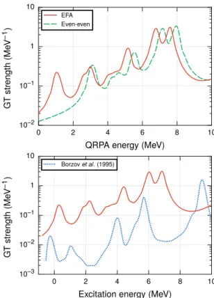
In Fig. 1, we plot the total Gamow-Teller strength function for the proton-odd nucleus71Ga. (In our EFA
calculation,71Ga has a slight deformationβ
2=−0.007;
our methods for extracting lab-frame transition strength from a deformed intrinsic nuclear ensemble are presented in the appendix). The top panel compares the strength functions obtained with the EFA-pnFAM and the even-even pnFAM, artificially constrained to obtain the correct odd particle number as suggested in Ref. [45]. The two calculations apply the same Skyrme energy-density func-tional (SV-min) without proton-neutron isoscalar pairing, but begin with distinct HFB calculations. The EFA cal-culation clearly includes important one-quasiparticle tran-sition strength nearEQRPA= 1 MeV that is not present
in the other calculation. The bottom panel compares the EFA-pnFAM strength, this time as a function of excita-tion energy in the daughter nucleus (shifted downward in energy by E0(pn) ' 749 keV—see Eq. (38) and the
discussion around Eq. (34)) with a finite Fermi system calculation from Ref. [46]. Although the two calculations
0 2 4 6 8 10
QRPA energy (MeV)
10–2 10–1 1 10
G
T
st
re
ng
th
(M
eV
–1)
EFA Even-even
0 2 4 6 8 10
Excitation energy (MeV)
10–3 10–2 10–1 1 10
G
T
st
re
ng
th
(M
eV
–1)
Borzovet al. (1995)
Figure 1. (Color online)Top panel: Gamow-Teller transition strength for71Ga, computed with the EFA-pnFAM (red, solid
lines) and the even-even pnFAM (green, dashed lines), after constraining the ground-state solution to have the correct odd average particle number, as in Ref. [45]. Bottom panel: The same EFA pnFAM strength function as in the top panel, plotted vs. excitation energyEex=EQRPA−E0(pn) (see (38)),
alongside the strength function from Ref. [46] (blue, dotted line).
do not yield identical strength functions, they clearly mirror one another, and both include low-energy one-quasiparticle strength.
Finally, the odd-Aformalism of Ref. [47], used by the authors of Ref. [17], is an approximate version of ours. We would recover similar expressions to those in Ref. [47] by substituting a separable Gamow-Teller interaction for the Skyrme interaction and dropping terms beyond leading order inPπν andQπν.
C. Application to β decay in deformed nuclei
Second, we apply theQ-value approximation of Ref. [7]:
Qβ= ∆Mn−H+λn−λp+E0(pn). (34)
Here ∆Mn−H is the neutron-Hydrogen mass difference, the λq are Fermi energies, andE0(pn) is the energy of
the lowest two-quasiparticle state for even-even nuclei, or the smallest one-quasiparticle transition energy for odd nuclei. We approximate E0(pn) with one-quasiparticle
energies from the HFB solution; this choice affects only Qβ, not the size of the QRPA energy window, which is determined as in Ref. [18]:
EQRPAmax =Qβ+E0(pn) =λn−λp+ ∆Mn−H. (35)
Our procedure for going from the intrinsic frame to the lab frame, generalized to include the odd-A EFA ensemble, is described in the appendix.
III. HALF-LIFE CALCULATIONS A. Identification of important nuclei
To identify the most importantβ-decay rates for weak and rare-earthr-process nucleosynthesis, we turn to two sets of nucleosynthesis sensitivity studies. Ref. [4] reviews sensitivity studies for mainr processes; our studies here proceed as described in Refs. [5,48,49] and Section 5.2 of the review, Ref. [4].
The rare-earth peak is formed in a mainr process, so for our first set of studies we begin with several choices of astrophysical conditions that produce a good match to the solarr-process pattern forA&120. These condi-tions include hot and cold parameterized winds, similar to those that may occur in core-collapse supernovae or accretion disk outflows, along with mildly heated neu-tron star merger ejecta. We run a baseline simulation for each astrophysical trajectory (i.e. condition) chosen, and then repeat it with individualβ-decay rates changed by a small factor, K. Individual β-decay half-lives in the rare-earth region tend to produce local changes to the final abundance pattern that influence the size, shape, and location of the rare-earth peak. Thus we compare the final abundances with those of the baseline simulation by using a local metric,flocal, defined as:
flocal(Z, N) = 100×
180
X
A=150
|YK(A)−Yb(A)|, (36)
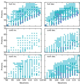
where Yb is the final baseline isotopic abundance, andYK is the final abundance in a simulation in which the β -decay rate of the nucleus withZ protons andN neutrons is multiplied by a factor K. Results for six studies, in which individualβ-decay rates were changed by a factor of K= 5, with hot, cold and neutron star mergerr-process conditions appear in Fig.2. The largest impacts to the final abundances occur near the peak (A∼160), though
50 55 60 65 70
Protons
hot inc hot dec
50 55 60 65 70
Protons
cold inc cold dec
90 95 100 105 110 115 120 Neutrons
50 55 60 65 70
Protons
nsm inc
90 95 100 105 110 115 120 Neutrons
nsm dec
Figure 2. (Color online) Influentialβ-decay rates in the rare-earth region for hot, cold, and mergerr-process conditions. The hot conditions are parameterized as in Ref. [50] with entropys/k= 200, dynamical timescaleτdyn = 80 ms, and
initial electron fraction Ye = 0.3; the cold conditions are parameterized as in Ref. [51] withs/k= 150,τdyn= 20 ms, andYe= 0.3; and the merger conditions are from a simulation of A. Bauswain and H.-Th. Janka, similar to that of Ref. [52]. We performed two sensitivity studies for each trajectory, looking at the results of increases and decreases to the rates by a factor ofK = 5. In order of lightest to darkest, the shades are: white (flocal= 0), light blue (0.1< flocal≤0.5), medium blue (0.5< flocal≤1.0), dark blue (1< flocal≤5), and darkest blue (flocal>5).
which nuclei are most sensitive depends a little on the astrophysical conditions chosen.
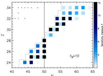
Figure 3. (Color online) Influentialβ-decay rates in theA∼80 region for weakr-process conditions, parameterized as in Ref. [50] with entropy per baryons/k = 10, dynamic timescale
τ = 200 ms, and starting electron fraction Ye = 0.3. The shaded boxes show the global sensitivity measures Fglobal
resulting fromβ-decay rate increases of a factor ofK = 10. Stability is indicated by crosses; theβ-decay rates of nuclei to the right of stability and to the left of the solid gray line have all been measured and so are not included in the sensitivity analysis.
a global sensitivity measureFglobal:
Fglobal= 100×X A
|XK(A)−Xb(A)|, (37)
whereXb(A) andXK(A) are the final mass fractions of the baseline simulation and the simulation with theβ-decay rate changed, respectively. Figure3shows representative results. The pattern of most influentialβ-decay lifetimes is similar to that identified for a mainr process [5]: the important nuclei tend to be even-N isotopes along either the r-process path or the decay pathways of the most abundant nuclei.
We select isotopic chains with the highest sensitivity measures, according to Figs.2 and3, and carefully re-calculate their β-decay half-lives. The selected chains encompass 70 nuclei in the rare-earth region and 45 nuclei in theA∼80 region1.
B. Selection and adjustment of Skyrme EDFs Our density-dependent nucleon-nucleon interactions are derived from Skyrme EDFs. Refs. [56–58] contain compre-hensive reviews of the properties of Skyrme functionals; Refs. [18,33] contain discussions of the most important
1 Measured half-lives of76,77Co and80,81Cu were recently reported
in Ref. [55]. We still include these nuclei in our calculations.
terms of the EDF for β decay. In our calculations, we largely apply the Skyrme EDF ‘as-is,’ but adjust a few important parameters that affect ground-state proper-ties and β-decay rates. Among these are the proton and neutron like-particle pairing strengths, Vp andVn; the spin-isospin coupling constant,C10s; and the
proton-neutron isoscalar pairing strength, V0. We tune these
parameters separately for each mass region; the coupling constants that multiply the remaining ‘time-odd’ terms of the Skyrme EDF are set either to values determined by local gauge invariance [58] or to zero.
1. Multiple Skyrme EDFs for the rare-earth elements
The pnFAM’s efficiency significantly reduces the com-putational effort in β-decay calculations. The smaller computational cost makes repeated calculations feasible and allows us to examine the extent to whichβ-decay predictions depend on the choice of Skyrme EDF. Here we use four very different Skyrme functionals: SkO0 [59], SV-min [60],unedf1-hfb [61], and SLy5 [62]. SkO0, has already been applied to theβ decay of spherical nuclei [7]; it was also chosen for the recent global calculations of Ref. [33]. SV-min, andunedf1-hfbare more recent; the latter is a re-fit of theunedf1parameterization [63], without Lipkin-Nogami pairing. SLy5 tends to yield less-collective Gamow-Teller strength than some other Skyrme parameterizations [64].
We do most of our calculations in a 16-shell harmonic os-cillator basis, a choice that further reduces computational time from that associated with the 20-shell basis applied in theunedfparameterizations of Refs. [63,65,66]. Be-causeunedf1-hfb was constructed with hfbtho in a 20-shell basis, however, we use this larger basis for that particular functional. We determine the nuclear deforma-tion by starting from three trial shapes (spherical, prolate, and oblate) and selecting the most bound result after the HFB energy and deformation have been determined self-consistently. We obtain the ground states of odd nuclei within the EFA, beginning from a reference even-even solution and then computing odd-A solutions for a list of blocking candidates reported byhfbtho. For odd-odd nuclei, we try allNp×Nn proton-neutron configurations to take into account as many odd-odd trial states as are practical. Again, we select the most-bound quasiparticle vacuum from among these candidates.
Returning to the functionals themselves: to adjust the pairing strengths and coupling constant C10s , we start from the published parameterizations.2 Then we fix the
2With a few exceptions: We use the same nucleon mass for proton
and neutrons, unlike Ref. [60], which originally determined SV-min, and we employ the SLy5 parameterization written into
hfbtho, which differs from that published in Ref. [62]. The
hfbtho values are the same as those of Ref. [67], but t0 =
Table I. OES indicators ˜∆(3)for the even-even nuclei used to
fit the pairing strengthsVpandVn.
Z N ∆˜(3)p (MeV) ∆˜(3)n (MeV)
52 84 0.79096±0.00464 0.75491±0.0024 54 86 0.90975±0.01527 0.87276±0.0022 56 90 0.92059±0.01093 0.92025±0.0204 58 90 0.99503±0.00975 0.97777±0.0092 60 92 0.68605±0.01176 0.77895±0.0298 62 94 0.57543±0.02887 0.67368±0.0042 62 96 0.55867±0.05021 0.58183±0.0049 64 96 0.57608±0.00276 0.67969±0.0018 66 98 0.53795±0.00277 0.67866±0.0016 68 100 0.55392±0.00312 0.64734±0.0017 68 102 0.50391±0.03646 0.60222±0.0021 70 104 0.52725±0.00300 0.53483±0.0017 72 106 0.62796±0.00168 0.63470±0.0016 72 108 0.62486±0.00388 0.57799±0.0022 74 110 0.55784±0.00199 0.66483±0.0008 74 112 0.60795±0.01224 0.70165±0.0013 74 114 0.67773±0.03607 0.79595±0.0227 76 116 0.78248±0.01110 0.83218±0.0020 78 118 0.75364±0.00128 0.88139±0.0009
like-particle pairing strengths Vp andVn by comparing the average HFB pairing gap to the experimental odd-even staggering (OES) of nuclear binding energies for the small set of test nuclei listed in Table I.3 Following
the procedure in Refs. [63, 65, 66], we adjust the HFB pairing gap to match the indicator (e.g., for neutrons)
˜
∆(3)n (Z, N) = 12[∆n(3)(Z, N+ 1) + ∆(3)n (Z, N−1)] for even-even nuclei. We obtain the usual three-point indicators ∆(3) [68,69] from mass excesses in the 2012 Atomic Mass Evaluation [70,71]—after using the prescription of Ref. [71] to remove the electron binding [65] from the atomic binding energies [72]. After finding pairing strengths that correspond to one-σuncertainties in ˜∆(3)(treating
asymmetric uncertainties as in Ref. [73]), we find best-fit valuesVpandVnfor our sample set of nuclei. For all EDFs except SV-min, we choose mixed volume-surface pairing, with α= 0.5 as in Ref. [18]. SV-min’s pairing piece was originally fixed along with the rest of the functional, but in the HF+BCS framework. We therefore re-fit the pairing strengths to better represent ground state properties with our HFB solver, keeping the coefficient that specifies density dependence at its value ofα= 0.75618 from Ref. [60].
Next, we determine an appropriate value for Cs
10 by
comparing the excitation energy,
Eex=EQRPA−E0(pn), (38)
of the Gamow-Teller giant resonance (GTR) to an experimentally-measured value in a nearby nucleus. This
3 The
unedf1-hfbpairing strengths were originally fit
simultane-ously with the rest of the functional (withhfbtho), so we do not re-adjust theunedf1-hfbpairing strengths.
0 5 10 15 20
Excitation energy (MeV)
0 5 10 15 20 25
G
am
ow
-T
el
le
rs
tre
ng
th
(M
eV
–1) Cs10(SkO′) = 128.0 MeV fm3
Cs10(SkO′-Nd) = 102.0 MeV fm3
Figure 4. (Color online) Gamow-Teller strength functions in
150
Pm for SkO0 (red dashed line, with Cs10 fit to the GTR
energy in208Pb) and SkO0
-Nd (purple solid line, withCs 10 fit
to the GTR energy in150Nd). The vertical line marks the measured GTR energy in150Pm.
constantCs
10 is the same one we adjusted to GTR data
in the past [18], following the work of Ref. [74]; Ref. [33] recently showed that it is the only particle-hole constant that is truly important forβ decay. In theseA ' 160 nuclei, we use the resonance associated with the doubly-magic nucleus208Pb, withEex= 15.6±0.2 MeV in the
odd-odd daughter208Bi [75], to fix it. We also use the
deformed rare-earth nucleus 150Nd (E
ex ' 15.25 MeV
in150Pm [76]), to fix an alternative valueCs
10 in SkO0,
calling the resulting functional SkO0-Nd. The two fits result in values ofC10s that differ by nearly 20%. Figure4 compares the Gamow-Teller strength functions produced by the two values in150Pm. Not only are the resonances
at different places, but there also a big difference in the strength functions at the low energies that are important forβ decay.
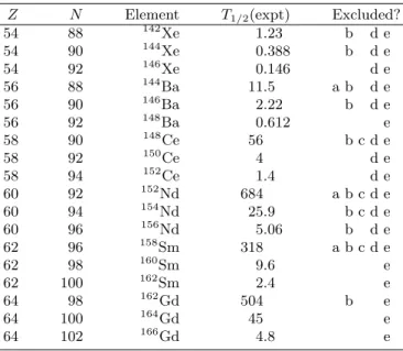
To adjust the T = 0 pairing, we select short-lived even-even isotopes withZ = 54, 56, 58, 60, 62, and 64 withβ-decay rates that have been measured reasonably precisely, according to Ref. [77]; the 18 nuclei we use are listed in TableII. For each nucleus, we attempt to find a pairing strengthV0that reproduces the measured half-life.
If a calculated half-life is too short, even when V0 = 0,
we remove the nucleus from consideration; this prevents our fit from being influenced by especially long-lived or sensitive isotopes. After determining an approximate V0 6= 0 for each nucleus (where possible), we compute
average of these values, weighing fast decays more than slow ones (since the very neutron-rich r-process nuclei are short-lived), with weight factors
wi =
1
log10
T1expt/2 (i)/35 ms. (39)
The fit is fairly insensitive to the weighting half-lifeT0=
35 ms; with T0 = 25 ms the fit values of V0 change by
Table II. Isotopes used to fit the proton-neutron isoscalar pairing to experimental half-lives from Ref. [77]. Labels a–e in the “Excluded?” column note which isotopes were excluded from the fits for the functionals (a) SkO0, (b) SkO0-Nd, (c) SV-min, (d) SLy5, and (e)unedf1-hfb, as discussed in the text.
Z N Element T1/2(expt) Excluded?
54 88 142Xe 1.23 b d e
54 90 144Xe 0.388 b d e
54 92 146Xe 0.146 d e
56 88 144Ba 11.5 a b d e
56 90 146Ba 2.22 b d e
56 92 148Ba 0.612 e
58 90 148Ce 56 b c d e
58 92 150Ce 4 d e
58 94 152Ce 1.4 d e
60 92 152Nd 684 a b c d e
60 94 154Nd 25.9 b c d e
60 96 156Nd 5.06 b d e
62 96 158Sm 318 a b c d e
62 98 160Sm 9.6 e
62 100 162Sm 2.4 e
64 98 162Gd 504 b e
64 100 164Gd 45 e
64 102 166Gd 4.8 e
Table III. Summary of proton-neutronT = 0 pairing fit, includ-ing the amount of test data in each fit (N) and the resulting pairing strength (V0).
EDF N V0
SkO0 15/18 −320.0
SV-min 14/18 −370.0
SkO0-Nd 9/18 −300.0
SLy5 6/18 −240.0
unedf1-hfb 0/18 −0.0
TableIII lists the values for V0 that we end up with
and the number of nuclei incorporated into the fit for each EDF. We find that none of the EDFs predict long-enough half-lives to fixV06= 0 for the entire set of test nuclei; SkO0
(15 of 18) and SV-min (14) come the closest, while SLy5 (only 6) andunedf1-hfb(zero) come less close and are thus poorly constrained byβdecay. (We discuss SkO0-Nd momentarily.) One cannot really have confidence in fits (SLy5,unedf1-hfb) that take into account less than half of the available data, but Fig.5provides at least a partial explanation. It compares our calculatedQvalues (34) to measured values [71] and those of the finite-range droplet model in Ref. [6]. Our Q values are almost uniformly larger than experiment (those of Ref. [6] are generally smaller), and those of SLy5 andunedf1-hfbare much larger. Because theβ-decay rate is roughly proportional to Q5 [78], a Q value that is too large will lead to an
artificially short half-life. TheT = 0 pairing only make the half-lives shorter.
TheQ-value fitting difficulties, however, do not
mani-142Xe144Xe146Xe144Ba146Ba148Ba148Ce150Ce152Nd154Nd156Nd158Sm160Sm162Gd –1.0
–0.5 0.0 0.5 1.0 1.5 2.0
Qβ
(c
al
c)
-Qβ
(e
xp
t)
(M
eV
)
Figure 5. (Color online) The difference between calculated and experimentalβ-decayQvalues, with SkO0 (circles), SV-min (diamonds), SLy5 (squares), andunedf1-hfb(triangles). Q
values of Ref. [6] (crosses) also appear.
fest themselves in actual half-life predictions as much as they might, even with SLy5 andunedf1-hfb. Figure6 compares our calculations to experimental measurements in the 18 test nuclei used to fit V0 (listed in Table II)
and an additional 18 rare-earth nuclei (listed in Table IV). Our results display the same pattern as many others (e.g., Refs. [17, 45, 79]), reproducing half-lives of short-lived nuclei better than those of longer-short-lived ones. The Q-value errors discussed previously show up as systematic biases in our half-life predictions (particularly with SLy5 andunedf1-hfb, for which half-lives of long-lived nuclei are artificially reduced). The shortest-lived nuclei, how-ever, are not so poorly represented even with SLy5 and
unedf1-hfb; these half-lives are still systematically short but by less than a factor of about two (the shaded region in Fig.6covers a factor of 5 relative to measured values). The systematic problems in the two functionals based on SkO0 are barely noticeable. SV-min, which performs the best overall, is somewhere in the middle. Because all the functionals do well with the short-lived isotopes, we use them all for our rare-earth calculations. The lifetimes we get withunedf1-hfb serve as lower bounds on our predictions.
Finally, although SkO0-Nd, the SkO0 variant that re-produces the GTR in 150Nd, fails in 9 of the 18 nuclei used for fitting, its predictions do not differ significantly from those of SkO0. Figure4 shows increased low-energy Gamow-Teller transition strength asCs
10 is reduced to
reproduce the rare-earth GTR. This increased low-lying strength reducesβ-decay half-lives so that a smaller pair-ing strength is required (see TableIII), with no loss of quality.
2. Weak r-process elements
Table IV. The 18 even-even rare-earth nuclei in Fig.6that are not included in the EDF fitting. Experimental half-lives are from Ref. [77].
Z N Element T1/2(expt)
50 84 134Sn 1.05
50 86 136Sn 0.25
52 82 134Te 2508
52 84 136Te 17.63
52 86 138Te 1.4
54 84 138Xe 844.8
54 86 140Xe 13.6
56 86 142Ba 636
56 94 150Ba 0.3
58 90 146Ce 811.2
62 90 156Sm 33840
66 102 168Dy 522
68 106 174Er 192
70 108 178Yb 4440
70 110 180Yb 144
72 112 184Hf 14832
72 114 186Hf 156
74 116 190W 1800
1 102 104 10–4
10–2 1 102 104
SkO′
1 102 104
SkO′-Nd
1 102 104
SV-min
1 102 104 10–4
10–2 1 102 104 SLy5
1 102 104
unedf1-hfb Experimental half-life (s)
Experimental half-life (s)
T1/
2
(c
al
c)
/
T1/
2
(e
xp
t)
T1/
2
(c
al
c)
/
T1/
2
(e
xp
t)
Figure 6. (Color online) Performance of fit functionals in even-even rare-earth nuclei. Filled symbols mark nuclei used to fit theT = 0 pairing. The experimental data are from Ref. [77].
best reproduces measured half-lives. Both Fig.6and the metrics in Ref. [17] point to SV-min as the best EDF. We adjust SV-min for these lighter nuclei in much the same way as discussed in the previous section. We fit the like-particle pairing to calculated OES values (see Table V), this time employing the fitting softwarepounders[80] to search for the best values ofVp andVn. We provide
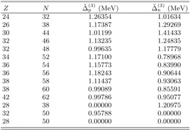
Table V. A' 80 nuclei used to fit the like-particle pairing strengths. We again use data from Ref. [71] to compute the experimental indicators ˜∆(3). We set ˜∆(3)= 0 for nuclei with
Z= 28 orN= 50.
Z N ∆˜(3)p (MeV) ∆˜
(3) n (MeV)
24 32 1.26354 1.01634
26 38 1.17387 1.29269
30 44 1.01199 1.41433
32 46 1.13235 1.24835
32 48 0.99635 1.17779
34 52 1.17100 0.78968
36 54 1.15773 0.83990
36 56 1.18243 0.90644
38 58 1.11437 0.93063
38 60 0.99089 0.85591
42 62 0.99786 0.95077
28 38 0.00000 1.20975
32 50 0.95788 0.00000
28 50 0.00000 0.00000
pounderswith the weighted residuals
Xi=wih∆¯i(Vp, Vn)−∆˜
(3)
i
i
, (40)
where ¯∆i is the average HFB pairing gap for the ith nucleus and the weight factorwi is 1 for non-magic nuclei and 10 for magic ones. The search yieldsVp =−361.0 MeV fm3 and V
n = −320.9 MeV fm3. We adjust the coupling constantC10s to the GTR in a lighter
doubly-magic nucleus,48Ca (E
ex= 10.6 MeV in48Sc [81]).
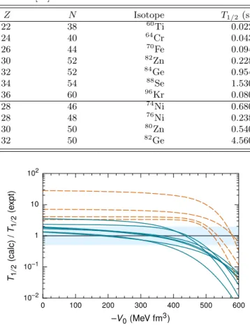
Finally, as before, we adjust theT = 0 pairing strength to reproduce measured half-lives of even-even nuclei, now withA'80 (see TableVI). In this region of the isotopic chart the fit is complicated by the presence of both proton and neutron closed shells (see Fig.3), so we includeZ= 28 andN= 50 semi-magic nuclei in the fit. Figure7shows the impact of the T = 0 pairing on half-lives and in particular in the difference in the effect between non-magic nuclei (solid lines) and semi-non-magic nuclei (dashed lines). We search for distinct values ofV0 for these two
cases, findingV0(nm) =−353.0 MeV fm3for non-magic
nuclei andV0(sm) =−549.0 MeV fm3 is for our set of
semi-magic nuclei.
The top panel of Fig. 8 shows the results of these adjustments, comparing calculatedβ-decay half-lives of even-even (left panel) and singly-odd (right) nuclei with measured values [82], for nuclei with 22< Z < 36 and T1/2<1 day. The bottom panel shows the same
compari-son for the finite-range droplet model (FRDM) calculation of Ref. [17]. The two sets of results are comparable, but those of Ref. [17] have a clear bias in even-even nuclei. A metric defined in Ref. [17],
ri= log10
"
T1calc/2(i)
T1expt/2 (i)
#
. (41)
captures the bias. The mean and RMS deviation of the tenth power ofri, called M10
Table VI. Open-shell (top) and semimagic (bottom) even-even
A'80 nuclei whose half-lives are used to adjust the proton-neutron isoscalar pairing. Experimental half-lives are from the ENSDF [82].
Z N Isotope T1/2(s)
22 38 60Ti 0.022
24 40 64Cr 0.043
26 44 70Fe 0.094
30 52 82Zn 0.228
32 52 84Ge 0.954
34 54 88Se 1.530
36 60 96Kr 0.080
28 46 74Ni 0.680
28 48 76Ni 0.238
30 50 80Zn 0.540
32 50 82Ge 4.560
0 100 200 300 400 500 600
–V0(MeV fm3) 10–2
10–1 1 10 102
T1/
2
(c
al
c)
/
T1/
2
(e
xp
t)
Figure 7. (Color online) Impact ofT = 0 pairing onβ-decay half-lives, both for non-magic (solid lines) and semi-magic (dashed lines) nuclei. The shaded region marks agreement between our calculation and measured half-lives [82] to within a factor of two.
deviation between calculation and experiment: A value M10
r = 2 would signify that calculations produce half-lives that are too long by a factor of two, on average. Our calculated rates yieldM10
r = 1.32 in even-even nuclei while those of Ref. [17] give M10
r = 3.55. For the standard deviation, our rates yield Σ10
r = 5.14, vs. 7.50 for those of Ref. [17]. Thus, we indeed do measurably better in even-even nuclei. Our results in odd-Anuclei are worse than those of Ref. [17], however; we obtainMr10 = 2.71 (vs. 0.95) and Σ10
r = 11.61 vs. (6.46). The two sets of calculations are comparable for short-lived odd-Anuclei, however: we getM10
r = 1.11 vs. 0.96 and Σ10r = 2.48 vs. 2.21 for isotopes withT1/2≤1 s.
C. Results near A= 160
Guided by the sensitivity studies in Fig.2, we identify 70 rare-earth nuclei, all even-even or proton-odd, with
10–4 10–2 1 102
104 This work
10–2 1 102 104 106 10–4
10–2 1 102
104 M¨olleret al. (2003)
10–2 1 102 104 106
Experimental half-life (s)
T1/
2
(c
al
c)
/
T1/
2
(e
xp
t)
Figure 8. (Color online) Performance of our SV-min calcu-lations (top panels) and the FRDM calcucalcu-lations of Ref. [17] (bottom panels) for nuclei with 22< Z < 36 and T1/2 ≤1
day. Left panels show the ratio of calculated to measured half-lives in even-even nuclei; right panels show the ratio in odd-A nuclei. Filled circles in the upper-left panel denote even-even nuclei used to fit theT = 0 proton-neutron pairing. The shaded horizontal band marks agreement to within a factor of five, and the white background marks nuclei with measured half-lives that are shorter than one second.
rates that strongly affectr-process abundances nearA= 160. (Neutron-odd nuclei do not significantly affect ther
process since they quickly capture neutrons to form even-N isotopes [1].) The top panels of Fig. 9present new calculated half-lives in two isotopic chains, with all five adjusted Skyrme EDFs. The bottom panels compare our half-lives to measured values where they are available [77], as well as to the results of previous QRPA calculations [17,33,83]. Our calculations span the (narrow) range of predicted half-lives in these isotopic chains, with SLy5 and unedf1-hfb predicting the shortest half-lives for the most neutron-rich isotopes, as one could expect from the analysis of Sec.III B 1. While theunedf1-hfb half-lives are uniformly short, however, those of SLy5 actually are actually the longest predictions (and the closest to measured values) for nuclei nearer to stability.
10–2 10–1 1 10 102 103
Z= 58 Z= 60
90 98 106 114 10–2
10–1 1 10 102 103
Z= 58
90 98 106 114 Z= 60
Neutron number
H
al
f-l
ife
(s
)
Figure 9. (Color online) Top panels: Half-lives for nuclei in the Ce (Z = 58, left) and Nd (Z = 60, right) isotopic chains, calculated with the Skyrme EDFs described in the text. Symbols correspond to the same EDFs as in Fig. 6. Bottom panels: Calculated half-lives of Refs. [17] (×), [33] (+), and [83] (?), measured half-lives [82] (circles), and the range of half-lives reported in this paper (shaded region).
half-lives, shorter than even those of unedf1-hfbmost of the time. Still, the band of predicted half-lives is relatively narrow among these three calculations even in the most neutron-rich nuclei. Ref. [33] points out that despite their differences, most global QRPA calculations produce comparable half-lives. Our results in bothA'80 and A'160 nuclei support this observation.
Finally, we have examined the impact of first-forbidden β decay on half-lives of rare-earth nuclei. Figure10shows that in heavier nuclei forbidden decay makes up between 10 and 40 percent of the total decay rate. The percentage generally increases withA.
D. Results nearA= 80
Following the weakr-process sensitivity study in Fig. 3, we present new half-lives for 45A'80 nuclei in Fig. 11, comparing our results to those of Refs. [17,33]. Not surprisingly, in light of Fig. 8, our calculated half-lives (circles) are often slightly shorter than those of Ref. [17] (crosses). They are also similar to those of Ref. [33], which used the same pnFAM code for even-even nuclei. We have also compared ourA'80 half-lives to those of the QRPA calculations in Ref. [79], finding very similar results for the few isotopic chains discussed both here and there.
One interesting feature of our calculation is that the half-lives of85,86Zn,89Ge, and (to a lesser extent)90As are long compared to those of Ref. [17]. The top panel of Fig. 12, which plots our calculated quadrupole deformationβ2
95 100 105 110 115 120
Neutron number
48 50 52 54 56 58 60 62 64 66
Pr
ot
on
nu
m
be
r
0% 10% 20% 30% 40% 50%+
Figure 10. (Color online) Impact of first-forbiddenβ transi-tions in rare-earth nuclei that are important for ther-process nuclei, with the Skyrme EDF SV-min.
forA'80 nuclei, suggests these longer half-lives are at least partially due to changes in ground-state deformation. The Zn isotopes switch from being slightly prolate to oblate near86Zn (N = 56), while Ge and As isotopes
do the same nearN = 57. Our calculations find 89Ge to be spherical and situated between two isotopes with β2 ∼ ±0.17. The authors of Ref. [17] appear to force 83−90Ge to be spherical.
The bottom panel of Fig.12shows the impact of first-forbiddenβ decay in this mass region; together with the top panel it connects negative-parity transitions with ground-state deformation. As discussed in Ref. [84], first-forbidden contributions toβ-decay rates are small, except in the oblate transitional nuclei discussed above. These results largely agree with those of the recent global calcu-lation in Ref. [33].
We also find that while the most deformed nuclei decay almost entirely via allowed transitions, spherical isotopes show a large scatter in the contribution of forbidden decay. More than 80 percent of the89Ge decay rate is driven
by first-forbidden transitions. This analysis may bear on the large first-forbidden contributions nearN= 50 and Z= 28 reported by Ref. [45], which restricted nuclei to spherical shapes. Ref. [79], which considers the effect of deformation on Gamow-Teller strength functions, suggests that it is important near this mass region.
44 46 48 10–3
10–2 10–1 1
H
al
f-l
ife
(s
)
Z= 24
46 48 50
Z= 25
46 48 50
Z= 26
49 50
Z= 27
51 52
Z= 29
54 56 10–3
10–2 10–1 1
H
al
f-l
ife
(s
)
Z= 30
55 57
Z= 31
54 56 58 60
Z= 32
56 58 60 62
Z= 33
58 60 62 64
Z= 34
Neutron number
Figure 11. (Color online) Computed half-lives inA'80β-decay (red circles), along with those of Refs. [33] (orange squares) and [17] (blue crosses).
apply the residue theorem to obtain integrated strength [85] we include (the negative of) spurious β+. Because
that strength is at low energy, it is strongly weighted by β-decay phase space. Of the 45 rates we calculate near A= 80, those for80,81Cu,86Ga,94As, and97Se may be
artificially small. This problem does not seem to appear in the rare-earth region.
IV. CONSEQUENCES FOR THE RPROCESS
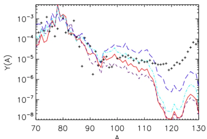
In rare-earth nuclei, our calculation produces rates that are either consistently larger than or smaller than (de-pending on the functional) those of, e.g., Ref. [17]. We now use these new rates in simulations of ther process. The resulting rare-earth abundances are shown in Fig. 13. Generally, calculations that predict low rates build up the rare-earth peak in both hot and coldr-process trajectories, and calculations that predict higher rates (SLy5 andunedf1-hfb) reduce the peak. Our neutron star merger calculation (bottom panel of Fig.13) demon-strates a different effect: longer-lived nuclei broaden the rare-earth peak, and shorter-lived nuclei narrow it. For all three trajectories the change in abundances is fairly localized, with the effects caused by our most reliable pa-rameterizations (SkO0, SkO0-Nd, and SV-min) modifying abundances by factors, roughly, of two to four.
NearA= 80, our calculations produce small changes in weakr-process abundances from those obtained with the β-decay rates of Ref. [17] and larger changes from
those with compilations. Fig.14shows the baseline weak
r-process calculation from the sensitivity study of Fig.3 (blue line), where theβ-decay lifetimes are taken from the REACLIB database [86]4 everywhere. We compare this
abundance pattern to those produced when theβ-decay rates for the set of 45 nuclei calculated in this work are replaced with our rates (red), those of Ref. [17] (purple), and those from Ref. [45] (teal). Although the differences in abundance produced by our rates and those of Ref. [17] are fairly small, differences produced by ours and those of Ref. [45] or REACLIB are noticeable, with the widely-used REACLIB rates producing the most divergent results. It appears that manyβ-decay rates nearA= 80 in the REACLIB database come from a much older QRPA calculation [87] that differs significantly from the more modern calculations, especially in lighter nuclei.
Even though many of our calculated rates are higher than those of Ref. [17] (Fig.11), their impact on a weak
r-process abundance pattern is not a uniform speeding-up of the passage of material through this region, as appears to be the case for for a mainr process (see, e.g., Ref. [7]). β-decay rates can influence how much neutron capture occurs in theA∼80 peak region and, consequently, how many neutrons remain for capture elsewhere [9]. Higher rates do not necessarily lead to a more robust weak r
process; in fact, the opposite is more usually the case, since more capture in the peak region generally leads to fewer
44 48 52 56 60 64
Neutron number
24 26 28 30 32 34
Pr
ot
on
nu
m
be
r
Quadrupole deformationβ2
44 48 52 56 60 64
Neutron number
24 26 28 30 32 34
Pr
ot
on
nu
m
be
r
Forbidden contribution (%)
–0.2 –0.1 +0.0 +0.1 +0.2
0% 10% 20% 30% 40% 50%+
Figure 12. (Color online)Top panel: Quadrupole deformation
β2 of the 45 A ' 80 nuclei whose half-lives we calculate
and display in Fig.11. Bottom panel: Contribution of first-forbiddenβ decay (0,1,2− transitions) to the decay rate of the same 45 nuclei, plotted as a percentage.
0.05 0.100.15 0.200.25 0.300.35
Y(A)
hot
0.05 0.100.15 0.200.25 0.300.35
Y(A)
cold
145 150 155 160 165 170 175 180 A
0.05 0.100.15 0.200.25 0.300.35
Y(A)
nsm
FRDM SkO'-Nd SkO' Sly5 SV-min UNEDF1
x 1.0e-04
Figure 13. (Color online) The effect of our newβ-decay rates on finalr-process abundances. The same trajectories are used as in Fig.2.
Figure 14. (Color online) Impact of ourβ-decay rates near
A= 80 on weakr-process abundances. The top panel shows abundances using rates from this work (red solid line), Ref. [17] (purple short dashes), Ref. [45] (light blue dot dashes), and the REACLIB database [86] (dark blue long dashes).
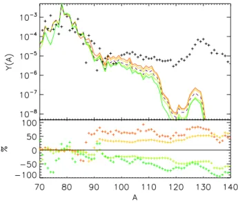
neutrons available for capture above the peak. This effect is illustrated in Fig.15, which compares the abundance pattern for the baseline weakr-process simulation from Sec. III A with those obtained by using subsets of our newly calculated rates in the same simulation. Consider first the influence of the rates of the iron isotopes (green line in Fig.15), particularly 76Fe. This N = 50 closed shell nucleus lies on ther-process path, below theN= 50 nucleus closest to stability along the path,78Ni. Thus an
increase to theβ-decay rate of76Fe over the its baseline
causes more material to move through the iron isotopic chain and reach the long waiting point at 78Ni. The
abundances near the A ∼ 80 peak increase and those above the peak region decrease because the neutrons used to shift material from the very abundant76Fe to78Ni are
no longer available for capture elsewhere. Changes to the β-decay rates of nuclei just above theN = 50 closed shell, however, can have a quite different effect on the pattern. The germanium isotopes, particularly86Ge and88Ge, are just above theN = 50 closed shell, so increases to their β-decay rates from the baseline will move material out of those isotopes to higherA(orange line in Fig. 15). Thus, abundances above the peak increase and more material makes it to the next closed shell,N = 82. In the end, the two very different effects partly cancel one another so that our rates do not change abundances significantly compared to those obtained with the rates of Ref. [17].
Figure 15. (Color online)Top panel: Final abundance pattern for the baseline trajectory described in the text, using the rates of Ref. [17] rates for all of the key nuclei identified in Sec. 2 (black line), compared to results of simulations with the same astrophysical trajectory and with new rates for68−72Cr only (light green line), new rates for72−76Fe only (green line), new rates for86−92Ge only (yellow line), and new rates for 89−95As only (orange line). Bottom panel: Percent difference
between the abundances produced by the baseline simulation (black line) and the simulations with the new rates (colored
lines).
rates by factors sampled from a log-normal distribution of width two and re-run the r-process simulation. Fig. 16shows the resulting finalr-process abundance pattern variances for 10,000 such steps. In each case, though some abundance pattern features stand out as clear matches or mismatches to the solar pattern, the widths of the main peaks and the size and shape of the rare-earth peak are not clearly defined. The real uncertainty inβ-decay rates is larger than a factor of two because all QRPA calcula-tions miss what could be important low-lying correlacalcula-tions. Thus, more work is needed, whether it be theoretical refinement or advances in experimental reach.
V. CONCLUSIONS
We have adapted the proton-neutron finite-amplitude method (pnFAM) to calculate the linear response of odd-A and odd-odd nuclei, as well as the even-even nuclei for which it was originally developed, by extending the method to the equal-filling approximation (EFA). The fast pnFAM can now be used to compute strength functions andβ decay rates in all nuclei.
After optimizing the nuclear interaction to best rep-resent half-lives in each mass region separately, we have calculated new half-lives for 70 rare-earth nuclei and 45 nuclei nearA= 80. Our calculated half-lives are broadly
Figure 16. (Color online) Ranges of abundance patterns pro-duced from Monte Carlo sampling of allβ-decay lifetimes from a log-normal distribution of width two in ther-process nuclear network, for hot (top panel), cold (middle panel), and merger (bottom panel) trajectories as in Ref. [88]. Points are solar
residuals from Ref. [2].
similar to those obtained in the global calculations of M¨olleret al. [17] as well as to those of more recent work. As a result,r-process abundances derived from our cal-culated half-lives are similar to those computed with the standard rates of Ref. [17]. Our calculations support the conclusions of Ref. [33], which compared multiple QRPA β-decay calculations and found that they all had similar predictions. Still, the comparison ofr-process predictions with much older ones in the REACLIB database and the discussion of uncertainty in Sec.IVdemonstrate the need for continued work on nuclearβ-decay.
ACKNOWLEDGMENTS
DE-FG02-02ER41216 (GCM), and DE-SC0013039 (RS). MM was supported by the National Science Foundation through the Joint Institute for Nuclear Astrophysics grant numbers PHY0822648 and PHY1419765 and under the auspices of the National Nuclear Security Administration of the U.S. Department of Energy at Los Alamos National Laboratory under Contract No. DE-AC52-06NA25396. We carried out some of our calculations in the Extreme Science and Engineering Discovery Environment (XSEDE) [89], which is supported by National Science Foundation grant num-ber ACI-1053575, and with HPC resources provided by the Texas Advanced Computing Center (TACC) at The University of Texas at Austin.
Appendix: Restoring Angular Momentum Symmetry Deformed intrinsic states like those we generate in
hf-bthorequire angular-momentum projection. Here we use
the rotor model [90,91], which is equivalent to projection in the limit of many nucleons or rigid deformation [34]. Even-even nuclei, with K = 0 ground states (K is the
intrinsicz-component of the angular momentum) are par-ticularly simple rotors. Their “laboratory-frame” reduced matrix elements are just proportional to full intrinsic ones [91],
hJ K||OˆJ||0 0i= ΘKhK|OˆJ K|0iintr, (A.1)
where ΘK = 1 for K = 0 and ΘK = √
2 for K > 0. The corresponding transition strength to an excited state |J Kiis
B( ˆOJ; 0 0→J K) = Θ2K hK|
ˆ
OJ K|0iintr
2
. (A.2)
FAM strength functions are essentially composed of squared matrix elements [29,85], so we simply multiply K >0 strength functions by Θ2K= 2.
The situation is more complicated in odd nuclei, which K 6= 0 ground-state angular momenta. The transfor-mation between lab and intrinsic frames, corresponding to Eq. (A.1), includes an additional term involving the time-reversed intrinsic state|Kii[91]:
hJfKf||Oλˆ ||JiKii=p2Ji+ 1h(JiKi;λ Ki−Kf|JfKf)hKf|Oλ,Kˆ f−Ki|Kiiintr
+ (Ji−Ki;λ Ki+Kf|JfKf)hKf|Oλ,Kˆ f+Ki|Kiiintr
i
.
(A.3)
If we neglect rotational energies in comparison with in- trinsic energies, we can sum overJi that appear in Eq. (A.3) to obtain [90]
B( ˆOλ; JiKi→Kf) = 1 2Ji+ 1
Ji+λ
X
Jf=|Ji−λ|
hJfKf||
ˆ
Oλ||JiKii
2
= hKf|
ˆ
Oλ,Ki−Kf|Kiiintr
2
+ hKf|
ˆ
Oλ,Ki+Kf|Kiiintr
2
.
(A.4)
The EFA-pnFAM, by preserving time-reversal symme-try and providing the combined transition strength from auxiliary states α†Λ|Φi and α†Λ¯|Φi, directly yields the
terms in Eq. (A.4). For example, the Gamow-Teller decay of a nucleus withJi=Ki = 3/2 involves, according to Eq. (A.4), three intrinsic transitions:
h3
2|OKˆ =0| 3 2i, h
5
2|OKˆ =1| 3 2i, h
1
2|OKˆ =−1| 3 2i.
The third matrix element is equivalent because of time-reversal symmetry toh−1
2|OKˆ =1| − 3
2i. Thus, a half-life
calculation to each band requires aK= 0 transition and
a pair ofK = 1 transitions from states|3
2iand | − 3 2i.
These are the auxiliary states that make up the EFA-pnFAM strength function. As a result, we obtain the total strength to a band in an odd nucleus the same way as in an even one: Stotal(F;ω) =SK=0(F;ω) + 2SK=1(F;ω) for
Gamow-Teller transitions. The calculation of forbidden strength is similar. The factor of two forK >0 strength cancels the factors of 1/2 that appear in the EFA strength function in (33). K = 0 transitions do not need this factor since, e.g.,K= 3/2→K= 3/2 andK=−3/2→ K=−3/2 transitions are equivalent and come together in the strength function.
[1] E. M. Burbidge, G. R. Burbidge, W. A. Fowler, and F. Hoyle, Reviews of Modern Physics29, 547 (1957).
450, 97 (2007),arXiv:0705.4512.
[3] S. Shibagaki, T. Kajino, G. J. Mathews, S. Chiba, S. Nishimura, and G. Lorusso, ApJ 816, 79 (2016), arXiv:1505.02257 [astro-ph.SR].
[4] M. Mumpower, R. Surman, G. McLaughlin, and A. Apra-hamian,Progress in Particle and Nuclear Physics86, 86 (2016).
[5] M. Mumpower, J. Cass, G. Passucci, R. Surman, and A. Aprahamian,AIP Advances4, 041009 (2014). [6] P. M¨oller, J. Nix, and K.-L. Kratz, Atomic Data and
Nuclear Data Tables66, 131 (1997).
[7] J. Engel, M. Bender, J. Dobaczewski, W. Nazarewicz, and R. Surman,Phys. Rev. C60, 014302 (1999). [8] O. L. Caballero, A. Arcones, I. N. Borzov, K.
Lan-ganke, and G. Martinez-Pinedo, ArXiv e-prints (2014), arXiv:1405.0210 [nucl-th].
[9] M. Madurga, R. Surman, I. N. Borzov, R. Grzywacz, K. P. Rykaczewski, C. J. Gross, D. Miller, D. W. Stracener, J. C. Batchelder, N. T. Brewer, L. Cartegni, J. H. Hamilton, J. K. Hwang, S. H. Liu, S. V. Ilyushkin, C. Jost, M. Karny, A. Korgul, W. Kr´olas, A. Ku´zniak, C. Mazzocchi, A. J. Mendez, II, K. Miernik, S. W. Padgett, S. V. Paulauskas, A. V. Ramayya, J. A. Winger, M. Woli´nska-Cichocka, and E. F. Zganjar,Physical Review Letters109, 112501 (2012).
[10] P. T. Hosmer, H. Schatz, A. Aprahamian, O. Arndt, R. R. Clement, A. Estrade, K.-L. Kratz, S. N. Liddick, P. F. Mantica, W. F. Mueller, F. Montes, A. C. Morton, M. Ouellette, E. Pellegrini, B. Pfeiffer, P. Reeder, P. Santi, M. Steiner, A. Stolz, B. E. Tomlin, W. B. Walters, and A. W¨ohr, Physical Review Letters 94, 112501 (2005), nucl-ex/0504005.
[11] P. Hosmer, H. Schatz, A. Aprahamian, O. Arndt, R. R. C. Clement, A. Estrade, K. Farouqi, K.-L. Kratz, S. N. Liddick, A. F. Lisetskiy, P. F. Mantica, P. M¨oller, W. F. Mueller, F. Montes, A. C. Morton, M. Ouel-lette, E. Pellegrini, J. Pereira, B. Pfeiffer, P. Reeder, P. Santi, M. Steiner, A. Stolz, B. E. Tomlin, W. B. Wal-ters, and A. W¨ohr, Phys. Rev. C 82, 025806 (2010), arXiv:1011.5255 [nucl-ex].
[12] C. Mazzocchi, R. Surman, R. Grzywacz, J. C. Batchelder, C. R. Bingham, D. Fong, J. H. Hamilton, J. K. Hwang, M. Karny, W. Kr´olas, S. N. Liddick, P. F. Mantica, A. C. Morton, W. F. Mueller, K. P. Rykaczewski, M. Steiner, A. Stolz, J. A. Winger, and I. N. Borzov,Phys. Rev. C
88, 064320 (2013).
[13] K. Miernik, K. P. Rykaczewski, R. Grzywacz, C. J. Gross, D. W. Stracener, J. C. Batchelder, N. T. Brewer, L. Cartegni, A. Fija lkowska, J. H. Hamilton, J. K. Hwang, S. V. Ilyushkin, C. Jost, M. Karny, A. Korgul, W. Kr´olas, S. H. Liu, M. Madurga, C. Mazzocchi, A. J. Mendez, II, D. Miller, S. W. Padgett, S. V. Paulauskas, A. V. Ra-mayya, R. Surman, J. A. Winger, M. Woli´nska-Cichocka, and E. F. Zganjar,Phys. Rev. C88, 014309 (2013). [14] K. Takahashi and M. Yamada,Progress of Theoretical
Physics41, 1470 (1969).
[15] S. Koyama, K. Takahashi, and M. Yamada,Progress of Theoretical Physics44, 663 (1970).
[16] K. Takahashi,Progress of Theoretical Physics45, 1466 (1971).
[17] P. M¨oller, B. Pfeiffer, and K.-L. Kratz,Phys. Rev. C67, 055802 (2003).
[18] M. T. Mustonen, T. Shafer, Z. Zenginerler, and J. Engel, Phys. Rev. C90, 024308 (2014).
[19] S. Perez-Martin and L. M. Robledo,Phys. Rev. C 78, 014304 (2008).
[20] R. Surman, J. Engel, J. R. Bennett, and B. S. Meyer, Phys. Rev. Lett.79, 1809 (1997).
[21] M. R. Mumpower, G. C. McLaughlin, and R. Surman, Phys. Rev. C85, 045801 (2012).
[22] M. R. Mumpower, G. C. McLaughlin, and R. Surman, The Astrophysical Journal752, 117 (2012).
[23] M. R. Mumpower, G. C. McLaughlin, R. Surman, and A. W. Steiner, ArXiv e-prints (2016),arXiv:1603.02600 [nucl-th].
[24] C. Fr¨ohlich, G. Mart´ınez-Pinedo, M. Liebend¨orfer, F.-K. Thielemann, E. Bravo, W. R. Hix, K. Langanke, and N. T. Zinner,Phys. Rev. Lett.96, 142502 (2006). [25] J. Pruet, R. D. Hoffman, S. E. Woosley, H.-T. Janka, and
R. Buras,The Astrophysical Journal644, 1028 (2006). [26] S. Wanajo,The Astrophysical Journal647, 1323 (2006). [27] F.-K. Thielemann, A. Arcones, R. K¨appeli, M. Liebend¨orfer, T. Rauscher, C. Winteler, C. Fr¨ohlich, I. Dillmann, T. Fischer, G. Martinez-Pinedo, K. Lan-ganke, K. Farouqi, K.-L. Kratz, I. Panov, and I. K. Korneev, Progress in Particle and Nuclear Physics66, 346 (2011).
[28] A. Arcones and F. Montes, ApJ 731, 5 (2011), arXiv:1007.1275 [astro-ph.GA].
[29] T. Nakatsukasa, T. Inakura, and K. Yabana,Phys. Rev. C76, 024318 (2007).
[30] P. Avogadro and T. Nakatsukasa,Phys. Rev. C84, 014314 (2011).
[31] M. Kortelainen, N. Hinohara, and W. Nazarewicz,Phys. Rev. C92, 051302 (2015).
[32] T. Nikˇsi´c, N. Kralj, T. Tutiˇs, D. Vretenar, and P. Ring, Phys. Rev. C88, 044327 (2013).
[33] M. T. Mustonen and J. Engel,Phys. Rev. C93, 014304 (2016).
[34] P. Ring and P. Schuck,The Nuclear Many-Body Problem (Theoretical and Mathematical Physics)(Springer, 2005). [35] J.-P. Blaizot and G. Ripka,Quantum Theory of Finite
Systems(The MIT Press, 1985).
[36] M. Stoitsov, N. Schunck, M. Kortelainen, N. Michel, H. Nam, E. Olsen, J. Sarich, and S. Wild, Computer Physics Communications184, 1592 (2013).
[37] N. Schunck, J. Dobaczewski, J. McDonnell, J. Mor´e, W. Nazarewicz, J. Sarich, and M. V. Stoitsov, Phys. Rev. C81, 024316 (2010).
[38] S. Perez-Martin and L. M. Robledo,Phys. Rev. C 76, 064314 (2007).
[39] A. L. Goodman,Nuclear Physics A352, 30 (1981). [40] H. Sommermann,Annals of Physics151, 163 (1983). [41] D. Vautherin and N. Mau,Nuclear Physics A422, 140
(1984).
[42] P. Ring, L. Robledo, J. Egido, and M. Faber,Nuclear Physics A419, 261 (1984).
[43] F. Alasia, O. Civitarese, and M. Reboiro,Phys. Rev. C
39, 1012 (1989).
[44] J. L. Egido and P. Ring,Journal of Physics G: Nuclear and Particle Physics19, 1 (1993).
[45] T. Marketin, L. Huther, and G. Mart´ınez-Pinedo,“Large scale evaluation of beta-decay rates of r-process nuclei with the inclusion of first-forbidden transitions,” (2015), arXiv:1507.07442.
[46] I. Borzov, S. Fayans, and E. Trykov,Nuclear Physics A
584, 335 (1995).