GENERALIZED FIDUCIAL INFERENCE FOR GRADED RESPONSE MODELS
Yang Liu
A dissertation submitted to the faculty of the University of North Carolina at Chapel Hill in partial fulfillment of the requirements for the degree of Doctor of Philosophy in the
Department of Psychology.
Chapel Hill 2015
c 2015 Yang Liu
ABSTRACT
YANG LIU: GENERALIZED FIDUCIAL INFERENCE FOR GRADED RESPONSE MODELS.
(Under the direction of David Thissen)
ACKNOWLEDGMENTS
I would like to show my gratitude to all the committee members, especially my academic advisors Drs. David Thissen and Jan Hannig. I could not have finished the work without their valuable feedbacks and advices. The project is sponsored by the Harold Gulliksen Psychometric Research Fellowship from the Educational Testing Service (ETS). I am grateful to my mentors Drs. Shelby Haberman and Yi-Hsuan Lee at ETS. It has been a great experience working under their supervision, and I have been greatly benefited from their expertise in statistics. In addition, I would like to offer my sincere appreciation to the help and support from the current and former members of the Thurstone Lab—especially Brooke, Jim, and Jolynn, and those from Hannig’s fiducial lab—Jessi, Qing, Dimitris, Abhishek, Rosie, and Jenny. I also cannot express enough thanks to Drs. Li Cai, Ji Seung Yang, and Scott Monroe for their continued support and encouragement for my work.
TABLE OF CONTENTS
LIST OF TABLES . . . ix
LIST OF FIGURES . . . x
1 INTRODUCTION . . . 1
1.1 Overview . . . 1
1.2 The graded response model . . . 2
1.2.1 Point estimation . . . 3
1.2.2 Confidence interval/set . . . 4
1.2.3 Goodness of fit testing . . . 5
1.3 Generalized fiducial inference . . . 7
2 THEORY . . . 16
2.1 A generalized fiducial distribution for item parameters . . . 16
2.2 A fiducial Bernstein-von Mises theorem . . . 24
2.3 Fiducial predictive inference. . . 27
2.3.1 Consistency . . . 28
2.3.2 Example: Response pattern scoring . . . 30
2.4 Goodness of fit testing with a fiducial predictive check (FPC) . . . 32
2.4.1 The centering approach . . . 33
2.4.2 The partial predictive approach . . . 33
2.4.3 Choice of test statistics . . . 35
3 COMPUTATION . . . 37
3.1 General structure . . . 37
3.2 Conditional sampling steps . . . 38
3.2.2 Conditional sampling ofZ?
id . . . 40
3.3 Updating interior polytopes . . . 42
3.4 Starting values . . . 45
3.5 Heavy-tailedness and a workaround . . . 46
3.6 Computational time. . . 48
4 MONTE CARLO SIMULATIONS. . . 50
4.1 Unidimensional models: Simulation design. . . 50
4.2 Unidimensional models: Parameter recovery . . . 54
4.3 Unidimensional models: Response pattern scoring . . . 62
4.4 Unidimensional models: Goodness of fit testing . . . 72
4.5 Bifactor models: Simulation design . . . 85
4.6 Bifactor models: Parameter recovery . . . 88
4.7 Conclusion . . . 93
5 EMPIRICAL EXAMPLE. . . 95
5.1 A unidimensional model . . . 96
5.2 A three-dimensional exploratory model . . . 99
5.3 A bifactor model . . . 101
5.4 Summary . . . 119
6 DISCUSSION AND CONCLUSION . . . 121
Appendix A BASIC PROPERTIES . . . 123
A.1 Calculating the fiducial density . . . 123
A.2 The invariance property . . . 124
Appendix B A BERNSTEIN-VON MISES THEOREM . . . 126
Appendix C NON-UNIQUENESS DUE TO SELECTION RULES . . . 137
Appendix D PREDICTIVE INFERENCE . . . 149
Appendix E FIDUCIAL PREDICTIVE CHECK . . . 150
LIST OF TABLES
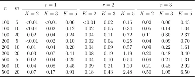
3.1 The average CPU time (in seconds) consumed by a single MCMC iteration under different combinations of sample size n, test length m, latent dimensionality r (exploratory model, minimally constrained), and number of categoriesK (Kj =K
for all j) . . . 49
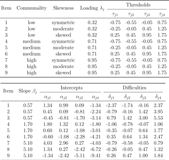
4.1 Data-generating parameter values for the unidimensional GRM (m = 9) . . . 52
4.2 Data-generating parameter values for the bifactor GRM (m = 9). . . 87
5.1 PROMIS emotional distress short-form items . . . 97
LIST OF FIGURES
1.1 The binomial proportion example . . . 12 2.1 Set inverse functions . . . 18 3.1 Trace plot for a slope parameter before and after implementing the workaround. . . 47 4.1 Empirical coverage and median length of CIs for unidimensional GRM parameters
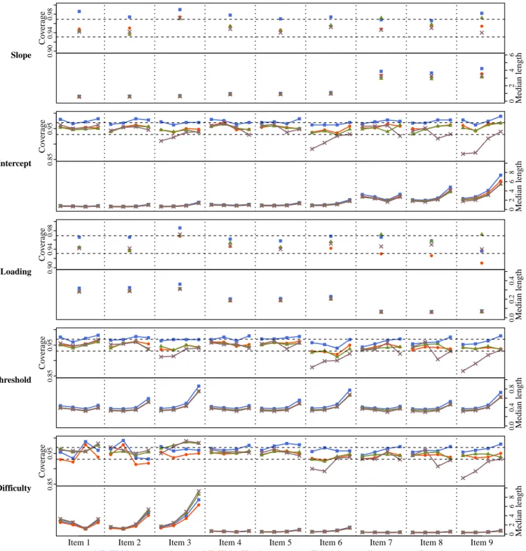
(n= 100, m= 9). . . 56 4.2 Empirical coverage and median length of CIs for unidimensional GRM parameters
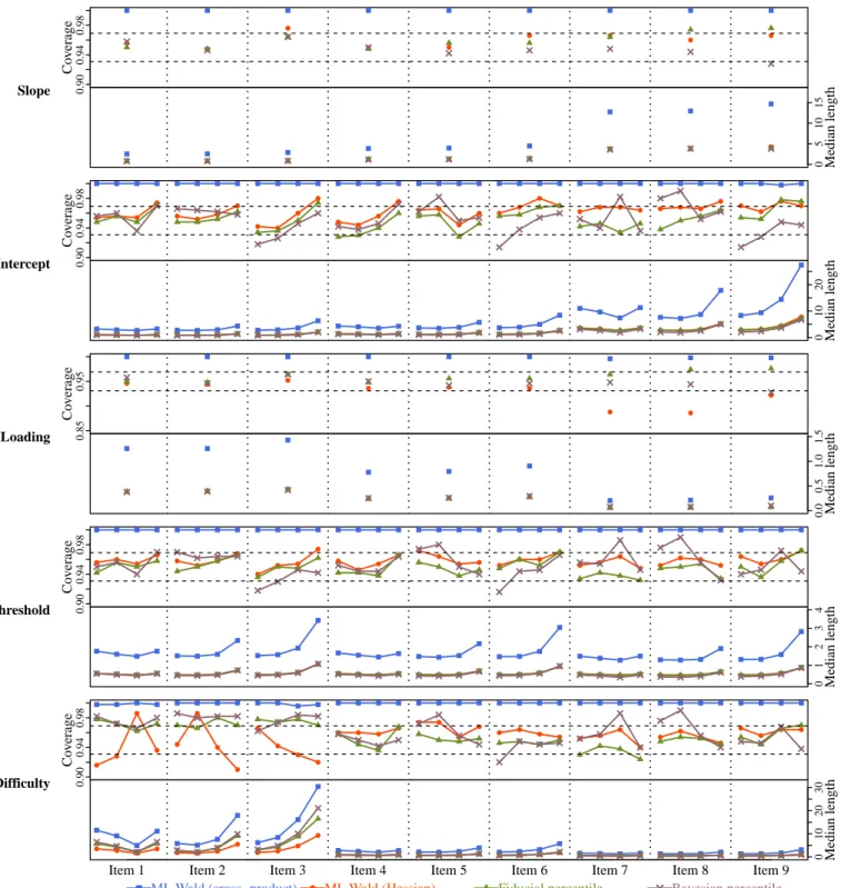
(n= 200, m= 9). . . 57 4.3 Empirical coverage and median length of CIs for unidimensional GRM parameters
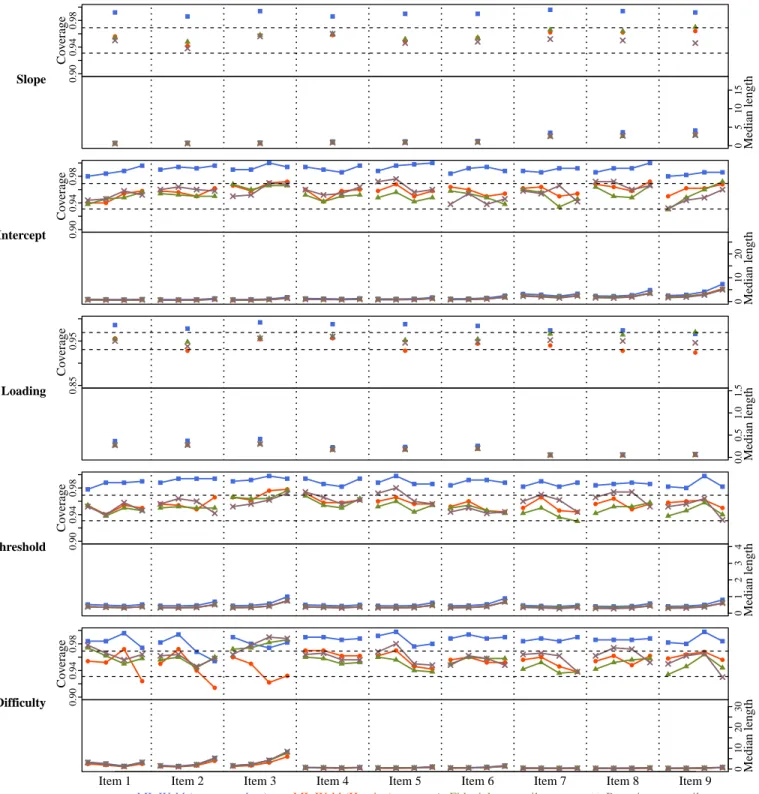
(n= 500, m= 9). . . 58 4.4 Empirical coverage and median length of CIs for unidimensional GRM parameters
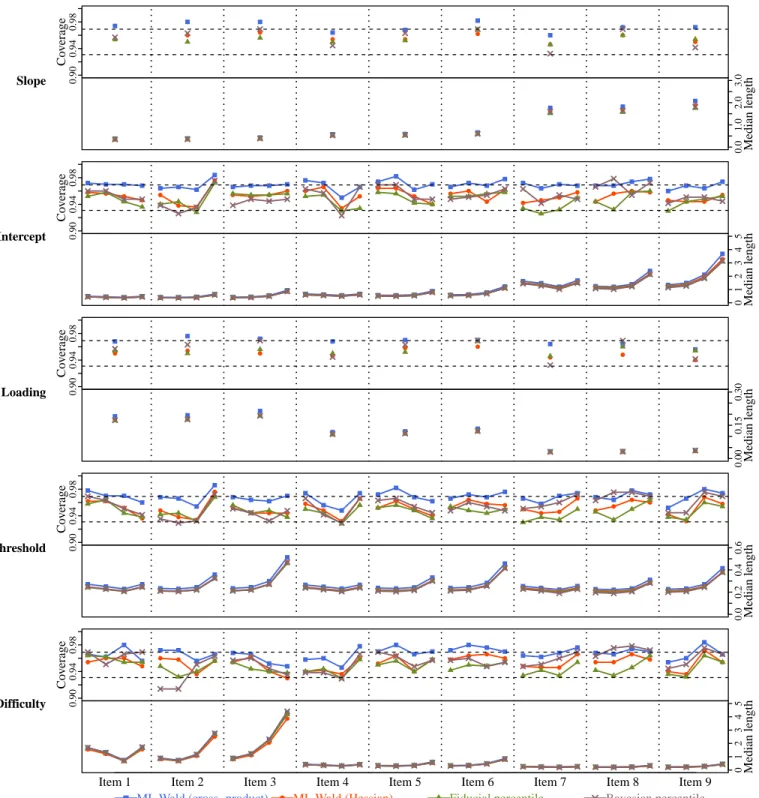
(n= 100, m= 18). . . 59 4.5 Empirical coverage and median length of CIs for unidimensional GRM parameters
(n= 200, m= 18). . . 60 4.6 Empirical coverage and median length of CIs for unidimensional GRM parameters
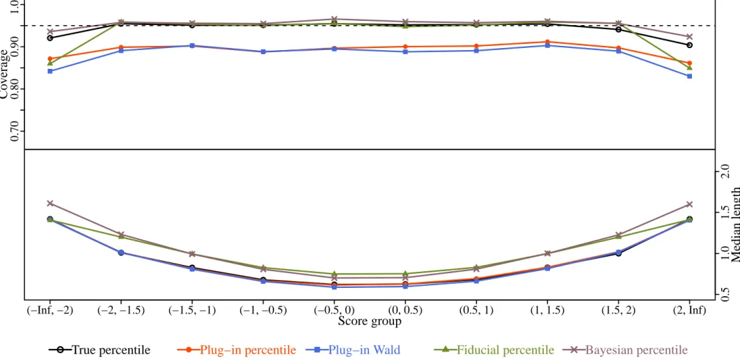
(n= 500, m= 18). . . 61 4.7 Empirical coverage and median length of prediction intervals for latent variable
scores (n= 100, m= 9). . . 65 4.8 Empirical coverage and median length of prediction intervals for latent variable
scores (n= 200, m= 9). . . 66 4.9 Empirical coverage and median length of prediction intervals for latent variable
scores (n= 500, m= 9). . . 67 4.10 Empirical coverage and median length of prediction intervals for latent variable
scores (n= 100, m= 18). . . 68 4.11 Empirical coverage and median length of prediction intervals for latent variable
4.12 Empirical coverage and median length of prediction intervals for latent variable scores (n= 500, m= 18). . . 70 4.13 Type I error results for score-group goodness of fit tests . . . 75 4.14 Type I error results for bivariate goodness of fit tests . . . 76 4.15 Power results for score-group goodness of fit tests: True model = 3-dimensional. . . 79 4.16 Power results for bivariate goodness of fit tests: True model = 3-dimensional . . . 80 4.17 Power results for score-group goodness of fit tests: True model = mixture . . . 82 4.18 Power results for bivariate goodness of fit tests: True model = mixture . . . 83 4.19 Empirical coverage and median length of CIs for bifactor GRM parameters (n =
200, m= 9). . . 89 4.20 Empirical coverage and median length of CIs for bifactor GRM parameters (n =
500, m= 9). . . 90 4.21 Empirical coverage and median length of CIs for bifactor GRM parameters (n =
200, m= 18). . . 91 4.22 Empirical coverage and median length of CIs for bifactor GRM parameters (n =
500, m= 18). . . 92 5.1 Fiducial predictivep-values for the sum-score group fit of the unidimensional GRM 98 5.2 Fiducial predictivep-values for the bivariate goodness of fit of the unidimensional
GRM . . . 103 5.3 Fiducial median and 95% fiducial percentile CIs for rotated factor loadings in the
three-factor EIFA . . . 104 5.4 Fiducial median and 95% fiducial percentile CIs for factor inter-correlations in
the three-factor EIFA . . . 105 5.5 Two-dimensional confidence regions for the primary and secondary loadings of
5.6 Two-dimensional confidence regions for the primary and secondary loadings of anxiety items . . . 110 5.7 Two-dimensional confidence regions for the primary and secondary loadings of
depression items . . . 111 5.8 Fiducial median and 95% confidence bands (CBs) of the marginal expected score
curve for general emotional distress. Pointwise and simultaneous CBs are shown in different colors.. . . 112 5.9 Fiducial medians and 95% confidence bands (CBs) of the marginal expected score
curve for anger. Only items in the anger subscale are shown here. Pointwise and simultaneous CBs are shown in different colors. . . 113 5.10 Fiducial medians and 95% confidence bands (CBs) of the marginal expected score
curve for anxiety. Only items in the anxiety subscale are shown here. Pointwise and simultaneous CBs are shown in different colors. . . 114 5.11 Fiducial medians and 95% confidence bands (CBs) of the marginal expected score
curve for depression. Only items in the depression subscale are shown here. Pointwise and simultaneous CBs are shown in different colors. . . 115 5.12 The fiducial median and 95% confidence bands (CBs) for marginal standard error
CHAPTER 1: INTRODUCTION
1.1 Overview
1.2 The graded response model
The graded response model (GRM; Samejima, 1969) has become a standard item re-sponse theory (IRT) model for analyzing Likert-type rere-sponse scales which have polytomous categories coded in order (e.g., strongly disagree, disagree, neutral, agree, strongly agree). Survey questionnaires including Likert items have been designed to measure many psycho-logical constructs including personality attributes, attitudes, health-related outcomes, etc. The GRM models responses to each item as an ordinal logistic regression (also known as a proportional odds model) on one or more latent variables representing the underlying constructs of interest. Heuristically, an item response is treated in the GRM as a discrete realization of a continuous but latent propensity that is related to individual differences in target constructs and also item characteristics. The relative position of a particular response category on the latent continuum is gauged by the adjacent item difficulty/intensity param-eters that are transformations of the slope and intercept paramparam-eters in the regression. The GRM reduces to the two-parameter logistic (2PL; Birnbaum, 1968) model when there are only two response categories.
In the current work, we focus our attention on a family of multidimensional logistic GRM models including unidimensional, bifactor, and exploratory GRMs as special cases. Our notation is more consistent with the mixed-effect modeling convention than the default choice in the IRT literature. For a Kj-category ordinal item j and a single respondent i,
define the item response function (IRF), denotedfj(θj, k|zi), as the probability of endorsing
the kth category, i.e., Yij = k, k = 1, . . . , Kj, conditional on this particular person’s latent
variable values Zi =zi:
fj(θj, k|zi) = P{Yij =k|Zi =zi}
=
1− 1
1 +eαj1+βj>zi, k = 0;
1
1 +eαj,Kj−1+βj>zi, k =Kj −1;
1
1 +eαjk+βj>zi −
1
1 +eαj,k+1+βj>zi, otherwise.
In (1.1), αjk’s denote the intercept parameters and βj the slopes. We assume that all the
intercept parameters are freely estimated, while some slopes are fixed for model identification; let θj be all free parameters that calibrate item j. The r-dimensional latent variables are
assumed to be standard normal, Zi ∼ N(0,Ir×r). Inference for models with unknown
covariance structure among latent dimensions (e.g., simple-structure models) is beyond the scope of the present work.
For a test comprising m graded items, we assume conditional dependence among item responses given the latent variable (e.g., McDonald, 1981), which implies the likelihood function f(θ,yi) of an individual item response vector yi = (yij)mj=1:
f(θ,yi) = Z
Rr
m
Y
j=1
fj(θj, yij|zi)dΦ(zi), (1.2)
in which Φ(·) denotes the probability measure of an r-dimensional standard normal distribu-tion. Further assume the sample is composed of n independent and identically distributed (i.i.d.) item response vectors y= (yi)n
i=1; the corresponding sample likelihood function is
fn(θ,y) = n
Y
i=1
f(θ,yi). (1.3)
1.2.1 Point estimation
dimensionality is high, however, approximation of the likelihood function based on tensor-product quadrature suffers from the well-known “curse of dimensionality” that the number of quadrature points grows exponentially fast. One solution given by Meng and Schilling (1996) is to incorporate a Gibbs sampler for the E-step computation, resulting in a Monte Carlo EM algorithm. Alternatively, Cai (2010a; 2010b) proposed approximation of the gra-dient of the log-likelihood function by a Metropolis-Hasting sampler and locating its zero by a Robbins-Monro-type search.
On the other hand, Bayesian methods based on stochastic approximations of the posterior distribution (e.g., Albert, 1992; Patz and Junker, 1999; Bradlow, Wainer, and Wang, 1999; Curtis, 2010; also see Edwards (2010) for its application in the GRM) are not affected as much by increasing latent dimensionality. Such a complex sampling problem is usually addressed by Markov chain Monte Carlo (MCMC) methods. However, it is commonly agreed that Bayesian methods are less user-friendly than ML: Statistical expertise is required to specify prior distributions and tune sampling algorithms. Even though the asymptotic optimality of Bayesian posteriors can be guaranteed by the celebrated Bernstein-von Mises theorem (e.g., Le Cam and Yang, 1986), erroneous results may be seen in finite-sample applications resulting from improperly chosen prior distributions or ill-behaved samplers.
1.2.2 Confidence interval/set
As a better alternative, CIs obtained by inverting the likelihood-ratio test have not yet been available in the IRT literature; the procedure itself is computationally intensive, and might not be suitable for multidimensional GRMs. Quantification of uncertainty for more complex transformations of parameters, e.g., the problem of drawing simultaneous confidence band on the item response functions (Thissen and Wainer, 1990) or information curves, are typically handled by less rigorous methods such as the bootstrap.
Bayesian methods based on posterior sampling are extremely flexible in terms of making inferences about arbitrary transformations of model parameters: One can apply the desired transformation to each Monte Carlo draw from the posterior distribution, leading naturally to a Monte Carlo sample of the transformed posterior. Moreover, we can save the random draws and pass them to subsequent analyses via, e.g., multiple imputation; compared to plugging in the point estimates, this accounts for the sampling variability in the initial model estimation stage. But the arbitrariness in prior selection may exert unpredictable influence on the finite-sample performance of Bayesian confidence sets, and thus they should be used with caution.
1.2.3 Goodness of fit testing
The item response data matrix y = (yij)ni=1mj=1 can be reorganized as an m-way
contin-gency table, in which each dimension corresponds to the Kj response categories of an item
and each cell of the table corresponds to a response pattern yi = (yij)mj=1. Therefore, it is
natural to assess GRM model fit by means of residuals in contingency table cells, testing whether the observed proportions are identical to the model-implied response pattern prob-abilities. For a general discussion on GOF testing for contingency table data, see Rao (1973, pp. 391-394) and more recently Haberman and Sinharay (2013). One salient feature of the item response data is sparseness, i.e., very small expected proportions for some cells, as a consequence of the number of cells, Qm
j=1Kj, increasing exponentially with the test length.
that the asymptotics are well suited to the resulting table of a smaller size; this has been termed the limited information approach by some authors. Existing GOF testing proce-dures in the IRT literature are mostly based on this rationale (e.g., Glas, 1988; Reiser, 1996; Maydeu-Olivares and Joe, 2005, 2006; Cai, Maydeu-Olivares, Coffman, and Thissen, 2006; Joe and Maydeu-Olivares, 2010; Cai and Hansen, 2013).
It is as important to identify the source of model misfit as to test the overall GOF of item response models. In practice, model modifications and/or item level fine-tuning should be performed before inferences can be safely drawn from the fitted GRM. When noa priori
information about the misfitting pattern is available, the source of misfit can be investigated by exploring the fit of the IRT model in low-dimensional (typically two-way or three-way) marginal subtables. For a comprehensive description of this approach, see Liu and Maydeu-Olivares (2014). If there is information about a potential violation of an assumption (e.g., conditional dependence, differential item functioning, etc.), researchers may specify a less restrictive model that reduces to the original model after imposing constraints, which turns the examination of model fit into a nested model comparison problem.
On the Bayesian side, posterior predictive checking (PPC; Guttman, 1967; Rubin, 1984) serves as a straightforward approach for detecting model misfit. When the model is correctly specified and the sample size is large enough, the value of a test statisticT(y) computed with the observed data set should be close to the same statistic computed from a predictive data set conditional on the posterior distribution of IRT model parameters. Here, the distribution of predictive data is a composite of the posterior distribution and the data-generating model, and thus can be approximated stochastically by drawing model parameters from the posterior and then simulating data conditional on these draws. For applications of PPC in IRT models, see Sinharay (2005), Sinharay, Johnson, and Stern (2006), and Levy, Mislevy, and Sinharay (2009).
a comprehensive estimation and inference framework that is able to: a) deal with high-dimensional latent traits, b) facilitate the assessment of uncertainty for various kinds of inference based on the model, and c) avoid as much subjectivity and ambiguity as possible in application. In the current research, generalized fiducial inference (GFI; Hannig, 2009, 2013) for a general class of multidimensional GRMs is proposed as an alternative to the existing full information methods. GFI satisfies most of the aforementioned desiderata. This recent variant of Fisher’s (1930, 1932, 1935) fiducial inference is an interesting theoretical middle ground between frequentist and Bayesian methods. Inferential procedures are based on a probability distribution supported on the parameter space, namely a fiducial distribution, which is derived using only the information contained in the data. Consequently, it inherits all the flexibility of Bayesian methods, but requires no prior knowledge of model parameters.
1.3 Generalized fiducial inference
Fisher (1930) put forward the notion of fiducial probability in response to the method of inverse probability (i.e., Bayesian inference, especially with a uniform prior), which in his view was “fundamentally false and devoid of foundation”. His concerns were conveyed in the following excerpt:
The peculiar feature of the inverse argument proper is to say something equivalent
to “We do not know the function Ψ specifying the super-population [i.e., the prior distribution of model parameters θ], but in view of our ignorance of the actual values of θ we may takeΨ to be constant.”. . . but however we might disguise it, the choice of this particular a priori distribution for the θ’s is just as arbitrary as any other could be.
He continued to point out that the claimed objectivity of the inverse probability cannot be translated under reparameterization:
If we were, for example, to replace our θ’s by an equal number of functions of them,
θ0
1, θ20, θ03, . . ., . . . all objective statements could be translated from the one notation to
a most complicated frequency function for θ0
1, θ20, θ30, . . .
He also summarized the major reason why inverse probability was popular—that is, quanti-fying uncertainty with probability is intuitive and handy, and Bayes’ rule seemed to be the only available tool at that time:
The underlying mental cause is. . . in the fact that we learn by experience, that science
has its inductive processes so that it is naturally thought that such inductions, being
uncertain, must be expressible in terms of probability. . . . The assumption was
al-most a necessary one seeing that no other mathematical apparatus existed for dealing
with uncertainties. . . . The introduction of quantitative variates [representing model parameters], having continuous variation in place of simple frequencies as the obser-vational basis, makes also a remarkable difference to the kind of inference which can
be drawn. . . . Inverse probability has, I believe, survived so long in spite of its
unsatis-factory basis, because its critics have until recent times put forward nothing to replace
it as a rational theory of learning by experience.
Fisher in his 1930’s article provided a template fiducial argument for a one-parameter model Y ∼ Fθ, in which θ is the parameter and Fθ is the distribution function
monoton-ically decreasing in θ, based on a single observation Y = y. By the probability integral transformation,Fθ(Y)∼Uniform(0,1), which is, in modern terminology, a pivotal quantity.
He transferred the pivotal distribution to the parameter space through function Fθ that is
considered a function of θ, equivalent to the operation of “de-pivoting” for the purpose of obtaining CIs with an exact coverage (see e.g., Casella and Berger, 2002). The resulting distribution, having density −dFθ/dθ, determines what Fisher called fiducial probability,
which in this case is the same as the correct coverage probability accumulated from repeated samples. Later, Fisher illustrated this approach again with a Gaussian variance example (Fisher, 1933), and generalized it to multidimensional parameters (Fisher, 1935).
summaries of the dispute. Moreover, Fisher’s interpretation of fiducial probability had been by no means cohesive: In his earlier work (Fisher 1930, 1933, and 1935), the fiducial prob-ability was largely treated as the synonym of frequent coverage as in the Neyman-Pearson repeated-sampling scheme (Neyman, 1934); however, a more epistemic view conceded to the Bayesian camp (Fisher, 1945, 1955) was adopted, at about the same time when he threw a heated polemic against Neyman. The confusion, according to Zabell (1992), was likely to be traced to Fisher’s mixed understanding of the nature of probability: In his own writings, probability is both “a frequency in an infinite hypothetical population” (Fisher, 1922) and “a numerical measure of rational belief” (Fisher, 1930). As a consequence, fiducial inference has been largely renounced by mainstream statisticians; it has been viewed as Fisher’s “one great failure” (Zabell, 1992) or “the biggest blunder” (Efron, 1998).
simple recipe to construct an asymptotic CD, namely the generalized fiducial distribution, which is adaptable to a broad collection of statistical models.
In brief, the goal of GFI is to find a fiducial distribution on the parameter space capturing all the information that the observed data conveys about model parameters. It is achieved by a role-switching between data and parameters similar to that involved in the definition of a likelihood function. Hannig’s (2009) fiducial argument operates on the data generating equation (also known as the structural equation):
Y =g(θ,U), (1.4)
which describes the data Y as a function of the parameters θ ∈Θ and random components
U having parameter-free distributions (i.e., pivotal quantities). For observed data Y = y, the data generating equation can be considered as an implicit function relating θ to U. Properly solving for θ from Equation 1.4, i.e., writing the parameters as a function of the data and random components, transfers the known distribution ofUto the parameter space and produces a fiducial distribution.
From now on, lowercase letters are routinely used for realizations of random variables. Let
Q(y,u) = {θ:g(θ,u) = y} (1.5)
denoted v(Q(y,u)), in which v(·) is some user-defined selection rule that chooses a point from the closure of Equation 1.5. On the other hand, when the set determined by Equation 1.5 is empty, it is similar to a linear system that has more equations than variables, in which case conflict may arise and no solution can be found. This implies that no feasible parameter value is able to recover y combined with the particular u. Because we assume the model is correctly specified, and thus at least the true parameter values should be contained in the set inverse, intuitively it means that thisu value is not helpful to the inference of θ and should be discarded. Therefore, we should always prevent this from happening, and one natural workaround is to concentrate on the set ofu such that Equation 1.5 is non-empty. Following these heuristics, a fiducial distribution can be defined as
v(Q(y,U?))| {Q(y,U?)6=∅}, (1.6)
in which U? is an independent and identically distributed (i.i.d.) copy of the data
generat-ing U. A (possibly vector-valued) random variable having the distribution determined by Equation 1.6 is referred to as a generalized fiducial quantity (GFQ), denoted R.
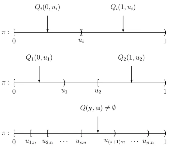
Next, we discuss an illustrative example, namely, the binomial proportion problem (see Dempster, 1966; Hannig, 2009). GFQ for the binomial proportion parameter is derived following the generic recipe; the derivation is in many aspects similar to that of our main problem described in the next chapter.
Example: Binomial proportion. SupposeY1, . . . , Yn are independent and identically
dis-tributed (i.i.d.) Bernoulli(π) random variables with success probability π. The data gener-ating equation for each Yi is
Yi =I{Ui ≤π}, Ui ∼Uniform(0,1), (1.7)
inverse of Equation 1.7:
Qi(yi, ui) =
[ui,1], if yi = 1;
[0, ui), if yi = 0.
(1.8)
Equation 1.8 is one of the two segments of interval [0,1] divided by the value of ui; see the
top panel of Figure 1.1 for a visualization.
π
:
[
)[
)
0
u
i1
Q
i(0
, u
i)
Q
i(1
, u
i)
π
:
[
)
[
)
0
u
1u
21
Q
1(0
, u
1)
Q
2(1
, u
2)
π
:
[
[
[
[
)
)
)
0
u
1:nu
2:n· · ·
u
s:nu
(s+1):n· · ·
u
n:n1
Q
(
y
,
u
)
6
=
∅
Figure 1.1: The binomial proportion example. The top panel shows the individual set inverse functionQi(yi, ui) foryi = 0 and 1, respectively. The middle panel gives an example of empty
Q(y,u) =Q1(y1, u1)∩Q2(y2, u2), in which y1 = 0, y2 = 1, and u1 < u2. The bottom panel
displays a non-emptyQ(y,u), in which the s=Pn
i=1yi smallestui’s, denoted u1:n, . . . , us:n,
correspond to successes, and the rest correspond to failures.
Let Y = (Yi)ni=1, and S =
Pn
i=1Yi ∼ Binomial(n, π). The set inverse function for Y,
denoted Q(y,u) in which u = (ui)ni=1, can be obtained by intersecting all individual set
it can be written as
Q(y,u) =
n
\
i=1
Qi(yi, ui) = [max
i:yi=1ui,i:yi=0min ui). (1.9)
The set defined by Equation 1.9 can be empty; an example is given in the middle panel of Figure 1.1. To obtain a non-empty intersection, we need maxi:yi=1ui < mini:yi=0ui, which
is illustrated in the bottom panel of Figure 1.1. Also let v(·) be a selection rule that yields an element of Equation 1.9. Thereby we define the generalized fiducial distribution of π following the generic recipe (Equation 1.6):
R=d v([max
i:yi=1U ? i,min
i:yi=0U ?
i))| {max i:yi=1U
?
i < min i:yi=0U
?
i}, (1.10)
in which U?
i’s are i.i.d. copies of Ui’s as usual. The GFD defined by Equation 1.10 satisfies
the stochastic ordering: Us:nRU(s+1):n, in which means “stochastically smaller than
or equal to”. More detailed discussion of this example, including the choice of selection rules v(·), can be found in Hannig (2009).
A GFQ serves as a prospective probabilistic quantification for the plausibility of model parameters after observing data, in contrast to the deterministic quantification given by the likelihood function, and also to the posterior distribution obtained by updating the prior knowledge of model parameters with the observed data. The fiducial probability of event {R ∈ A ⊂ Θ} corresponds to the long-run proportion that parameter values in A would be needed in order to reproduce the observed data y, over repeated data generation from the model (i.e., generate U? from its parameter-free distribution). Here we ignore
for a general discussion). A different connection between the two is established later for our problem involving a marginal likelihood, similar to that given by Liu and Hannig (2014, Remark 3).
GFQs defined by Equation 1.6 suffers from three major sources of non-uniqueness (Han-nig, 2009): a) the choice of data generating equations, b) the choice of selection rules, and c) conditioning on a set with probability 0 (i.e., the Borel paradox, see Proschan and Presnell (1998) for detailed discussions). In the application of GFI to the GRM, we use a simple and natural data generating equation that parallels the way graded item response data are typi-cally simulated in Monte Carlo studies, and that is shown to lead to a fiducial distribution that satisfies a Bernstein-von Mises theorem (and consequently an asymptotic CD); there-fore, we do not feel pressed to explore other possible data generating equations. In addition, c) does not apply to categorical data, so it will not be discussed either. For b), it can be shown that the diameter of the set given by Equation 1.5 in our problem shrinks to 0 at the rate 1/n, faster than the rate 1/√n at which GFQ approaches its normal limit as dictated by the Bernstein-von Mises theorem. Non-informative and data independent selection rules are recommended by Hannig (2009, Section 7) for finite sample applications.
In practice, Monte Carlo methods are frequently used when GFI is applied to complex parameteric models, due to fact that exact computation of functionals of the fiducial distri-bution, e.g., median and quantiles, are often intractable. The target distribution (Equation 1.6) can be approximated by simulating U? subject to the constraint Q(y,U?) 6= ∅ and
constructing the implied set inverse Q(y,U?) from each Monte Carlo draw of U?, which is
CHAPTER 2: THEORY
In this chapter, we derive a generalized fiducial distribution of item parameters under the family of multidimensional graded response models (GRMs; characterized by Equation 1.1). A Bernstein-von Mises theorem is established to justify the asymptotic correctness of generalized fiducial inference (GFI) for making inferences about item parameters and their transformations. We also discuss the consistency of the fiducial predictive distribution for sample statistics whose distributions depend on the item parameters, which is applicable to constructing predictive intervals for response pattern scores. We conclude this section by discussing an easy-to-implement goodness of fit testing procedure, the fiducial predictive check (FPC), analogous to the posterior predictive check (Guttman, 1967; Rubin, 1984) in the Bayesian literature.
2.1 A generalized fiducial distribution for item parameters
Following the general recipe introduced in Chapter 1, we derive a generalized fiducial distribution for item intercepts and slopes given independent and identically distributed (i.i.d.) responses to a collection of graded items. We start from the data generating equation of a person’s response to an item under the GRM, and find the set inverse function of item parameters corresponding to this particular data entry. Combining all individual set inverse functions, we arrive at the set inverse for the entire item response data set, based on which a fiducial distribution can be defined in the form Equation 1.6.
Conditional on the latent variable Zi, person i’s response to item j, i.e., Yij, follows
a multinomial distribution with probabilities P{Yij = k|Zi} = fj(θj, k|Zi), k = 1, . . . , Kj,
and βj are collected inθj. Similar to the binomial proportion example discussed in the
pre-vious chapter, the data generating equation (e.g., Hannig, 2009, Example 5) of the ordinal Yij can be written as
Yij = Kj−1
X
k=1
I{Uij ≤fj(θj, k|Zi)}= Kj−1
X
k=1
I{Aij ≤αjk +βj>Zi}, (2.1)
in which Uij ∼ Uniform(0,1), Aij = logit(Uij) ∼ Logistic(0,1), and Zi ∼ N(0,Ir×r). Here,
Aij and Zi can be identified as the pivotal componentU in the general formulae (equations
1.4 to 1.6). Assumerj slopes are free (rj ≤r), and thus the dimension ofθj isqj =rj+Kj−1;
in the sequel, we only consider the case in which the fixed slopes are zero for simplicity1. The
set inverse function of Equation 2.1 is the following subset of the qj-dimensional parameter
space:
Qij(yij, aij,zi) = {θj ∈Rqj :aij > αj1+βj>zi, if yij = 0;
aij ≤αj,K−1+βj>zi, if yij =K;
αj,k+1+βj>zi < aij ≤αjk+βj>zi, otherwise.}
(2.2)
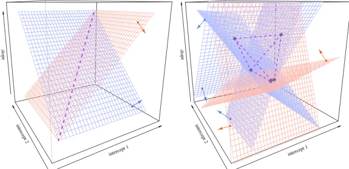
Geometrically, Equation 2.2 corresponds to the intersection of two half-spaces ifk is a middle category, and a single half-space if k = 0 or Kj −1. A graphical illustration of Equation
2.2 for a three-category item is given in the left panel of Figure 2.1, in which the parameter space is three dimensional (two intercepts and one slope).
The set inverse function for n i.i.d. responses to itemj, denoted Y(j) = (Yij)ni=1, is given
1In practice, slopes might be fixed at values other than zero. The theoretical properties discussed in the
current work still apply after subtracting the inner product of those fixed slopes and the corresponding normal variates from Aij’s and substituting its distribution function for the standard logistic cumulative
intercept 1 intercept 2
slope
intercept 1 intercept 2
slope
Figure 2.1: Set inverse functions for a single response entry Yij (left) and five i.i.d.
re-sponses (right) for a 3-category graded item. Colors of the wireframes indicate directions of inequality signs, and arrows point into the corresponding half-spaces. On the left, the purple-colored dashed line gives a boundary of the parameter spaceαj1 =αj2. On the right,
the intersection of all half-spaces is shown as the polytope surrounded by its purple-colored edges and highlighted vertices
by the intersection of all individual set inverse functions (Equation 2.2):
Qj(y(j),a(j),z) = m
\
j=1
Qij(yij, aij,z) (2.3)
in which a(j) = (aij)ni=1 and z = (zi)ni=1 are realizations of the logistic and normal random
variables. We take the intersection for a reason similar to that discussed in the binomial proportion example: Because the same intercept and slope parameters appear in the data generating equations of allnresponses (Yij)ni=1, the set inverse should contain values of those
item parameters that are consistent with all the equations. The right panel of Figure 2.1 depicts the set inverse for five responses to the same three-category item: A three-dimensional closed polyhedron is obtained as the intersection of the corresponding half-spaces.
Finally, consider a sample of i.i.d. responses Y = (Yi)n
m graded items. Because we assume that items do not share parameters, the set inverse function for the entire set of item response data
Q(y,a,z) =
m
×
j=1Qj(y(j),a(j),z) (2.4)
is a subset of the entire parameter space Θ⊂Rq1×· · ·×
Rqm, in which×denotes the Cartesian
product. A generalized fiducial distribution can be constructed following the general recipe (Equation 1.6):
v(Q(y,A?,Z?))| {Q(y,A?,Z?)6=∅}, (2.5)
in which v(·) denotes some user-defined rule that selects one point from each item’s poly-hedron. A? and Z? are i.i.d. copies of A and Z, respectively; again, the asterisks are used
to distinguish them from their data-generating counterparts. Note that bothA? and Z? are
continuous random variables, and thus we do not differentiate Q(y,A?,Z?) from its closure:
i.e., the polyhedrons with attained boundaries. In the sequel, call a random variable follow-ing the distribution given by Equation 2.5 a generalized fiducial quantity (GFQ), denoted
R.
In finite samples, the polyhedron implied by Equation 2.3 is not necessarily bounded; for example, when n ≤ qj, it is certainly unbounded, because a bounded polytope on the
qj-dimensional space has at leastqj+ 1 faces. We require a finite point being returned by the
selection rule: i.e., |v(Q(y,a,z))| <∞ for all y, aand z such thatQ(y,a,z) is non-empty; hence, infinity is not included in the support of the resulting fiducial distribution (Equation 2.5) in unbounded cases. Eventually, the polyhedrons become bounded as the sample size tends to infinity; it is in fact a corollary of Theorem 2 which states a stronger property that the diameter of the set inverse shrinks to zero at a fast rate.
In addition, it is plausible that the set inverse (Equation 2.4) touches the boundary of the parameter space imposed by the ordering of item intercepts, i.e., ∂Θ = {θ : αjk =
there exists more than one endorsement to a response categorykof itemj, e.g.,y1j =y2j =k,
then αj,k+1 < min{A?1j −βj>Z?1, A?2j −βj>Z?2} ≤ max{A?1j −βj>Z?1, A?2j −βj>Z?2} ≤ αjk,
with a strict inequality attained almost surely by the continuous nature of the logistic and normal variates. As long as the data-generating values of the item parameters are in the interior of the parameter space, all the response patterns happen with a positive probability, and thus the set inverse is eventually bounded away from ∂Θ with probability one.
Some extra notation is introduced. Let τjk(θj,zi) =αjk +βj>zi be the linear regression
on the latent variable. Also set τj0(·,·) = ∞ and τjKj(·,·) = −∞ by convention; with the
help of these notations, we simplify the IRF (Equation 1.1) to
fj(θj, k|zi) =
1
1 +e−τjk(θj,zi) −
1
1 +e−τj,k+1(θj,zi), (2.6)
and the set inverse function (Equation 2.2) to
Qij(yij, aij, zi) = {θj ∈Rqj :τj,k+1(θj,zi)< aij ≤τjk(θj,zi)}. (2.7)
Consideryfixed for now. Each vertex of the possibly unboundedRqj-polyhedronQj(y(j),a(j),z)
residing in the interior of Θ is the solution of a set of qj linear equations of form aij =
τjk(θj,zi), contributed from qj observations and some suitable choices of left/right bounds
depending on the responses of those selected observations2. Notationally, let I
j be a size-qj
sub-sample of observations. Also let kIj = (kij)i∈Ij be an index tuple of length qj, each
element of which kij ∈ {yij, yij + 1} indicates whether the right half-space aij ≤τjyij(θj,zi)
or the left half-space τj,yij+1(θj,zi) < aij is selected for each i ∈Ij3. Only a small fraction
of (Ij,kIj) pairs are needed to determine a vertex: It only happens when the qj boundary
hyperplanes of the selected half-spaces are finite and produce a non-singular linear system.
2If an observation contributes two equations, then the resulting vertex is on the boundary of Θ. This happens
with probability zero for sufficiently largen.
3Here, I
Suppose a fixed non-empty set inverse function Qj(y(j),a(j),z) has vj vertices; they can be
indexed by a collection of properly selected pairs Pj ={(Ij(l),kI(l) j )}
vj
l=1. Pooling across all m
items in the test, write I =Sm
j=1Ij, kI = (kIj)mj=1, and P =
×
mj=1Pj;P indexes all extremal
points of the set inverse Q(y,a,z) for the entire set of item response data.
We first consider selection rules that yield interior extremal points of Q(y,A?,Z?) and
are independent of A? and Z?, for which the resulting fiducial density has a closed-form
expression. Write the selected point V = (Vj)m
j=1 = v(Q(y,A?,Z?)), in which Vj is the
selected vertex of polyhedron Qj(y(j),A?(j),Z?). For each item j, letVIj,kIj be the solution
determined by a particular sub-sampleIj together with a particular combination of left/right
boundskIj, and EIj,kIj be the event thatVIj,kIj gives an interior vertex ofQj(y(j),A?(j),Z?).
Also let VI,kI = (VIj,kIj) m
j=1, EI,kI denote the event that VIj,kIj determines an extremal
point of Q(y,A?,Z?), and E
P denote the event that all the extremal points are indexed by
P. The generic fiducial quantity (Equation 2.5) associated with a selected extremal point of the set inverse function (Equation 2.4) is given in the following lemma; see Appendix A for the derivation, which is similar in spirit to the proof of Lemma A.1 and B.1 in Hannig (2013), the first part of Theorem 1 in E et al. (2009), and Lemma 1 in Liu and Hannig (2014).
Lemma 1. Consider m graded items each of which is characterized by equation 2.6. Let
Θ⊂ Rq1 × · · · ×Rqm be the parameter space of item parameters θ, comprising all free item intercepts and slopes. We observe i.i.d. ordinal item response data y = (yi)n
i=1, in which
each response category of each item has more than one endorsement. Then, the density of
written as4
gn(θ|y)∝
X
I
X
kI
wI,kI(y)
· Z
Rnr
m
Y
j=1
dIj,kIj(θj,zIj)·
Y
i∈Ij
eτjkij(θj,zi)
[1 +eτjkij(θj,zi)]2
·Y
i∈Ic j
fj(θj, yij|zi)
dΦ(z). (2.8)
In Equation 2.8, dIj,kIj(θj,zi) =
det(∂τjkij(θj,zIj)/∂θj)i∈Ij
, zIj = (zi)i∈Ij, Φ(·) denotes a
standard normal probability measure5, and
wI,kI(y) =P{V=VI,kI|EI,kI}
∝ X
P3(I,kI)
P{V =VI,kI|EP} ·P{EP} (2.9)
is contingent upon P{V =VI,kI|EP}, i.e., the specific selection rule being used.
Remark 1. The connection between GFI and Bayesian inference can be seen from Equation 2.8. As a general notation, we put index set in subscript to denote the corresponding
4The sum on the right-hand side of Equation 2.8 is taken over all combinations ofIandk
I. Some of (Ij,kIj) pairs are not able to produce a vertex; in those cases, the Jacobian determinantdIj,kIj is zero, and thus the corresponding summand in Equation 2.8 vanishes.
elements: e.g., zI = (zi)i∈I. Rewrite Equation 2.8 by splitting the integral into two parts—
one for zI, and the other for zIc:
gn(θ|y)∝
X
I
X
kI
wI,kI(y)
Z m Y
j=1
dIj,kIj(θj,zi)
·Y
i∈I
Y
j∈J(i)
eτjkij(θj,zi)
[1 +eτjkij(θj,zi)]2
Y
j /∈J(i)
fj(θj, yij|zi)
dΦ(zI)
· Z
Y
i∈Ic m
Y
j=1
fj(θj, yij|zi)dΦ(zIc), (2.10)
in which J(i) = {j : i ∈ Ij} for i ∈ I. Note that the last line of Equation 2.10 is the
marginal likelihood function of the remaining observations Ic. We can multiply and divide
the right-hand side of Equation 2.10 by the likelihood of the vertex-determining observations I, and then simplify it to
gn(θ|y)∝bn(θ,y)fn(θ,y). (2.11)
In Equation 2.11,
fn(θ,y) =
Z n Y i=1 m Y j=1
fj(θj, yij|zi)dΦ(z), (2.12)
denotes the complete sample likelihood, and
bn(θ,y) =
X
I
X
kI
wI,kI(y)
Z m Y
j=1
dIj,kIj(θj,zIj)
Y
i∈I
Y
j∈J(i)
eτjkij(θj,zi)
[1 +eτjkij(θj,zi)]2
Y
j /∈J(i)
fj(θj, yij|zi)
dΦ(zI) Z
Y
i∈I m
Y
j=1
fj(θj, yij|zi)dΦ(zI). (2.13)
the (empirical) Bayesian posterior computed from the data-dependent prior proportional to Equation 2.13.
To simplify the proof of our main theorem (Theorem 1), we impose a further restriction on the selection rules: Whenever I 6= I0 but yI = yI0 and kI = kI0, it is required that
wI,kI(y) = wI0,kI0(y); the common function value is denoted bywyI,kI(y). It implies that the
number of distinct values of wyI,kI(y) does not grow with the sample size, because yI and kI have only finitely many patterns. A simple selection rule that satisfies such condition, which is also recommended in actual computation, is to select with equal probability among the interior vertices of each polyhedron Qj(y(j),A?(j),Z?).
The next result implies that the fiducial density (Equation 2.8) is invariant under smooth transformations, similar to the invariance of the Bayesian posterior derived from the Jeffreys prior. This is a desirable property because inference about item parameters remains the same when the model is re-parameterized. For example, researchers may be interested in the alternative slope-difficulty or the standardized loading-threshold parameterizations of the GRM model, and inference can be safely drawn about those transformed parameters using the correspondingly transformed generalized fiducial distributions. Definitions of those specific transformations are provided later in Chapter 4.
Proposition 1 (Invariance). Let θ = q(ξ) be a one-to-one and continuously differentiable function onto the parameter space Θ. Denote the data generating equation corresponding to Equation 2.8 by Y = g(θ,A,Z), and write g˜n(ξ|y) as the generalized fiducial distribution
computed from the data generating equation Y = g(q(ξ),A,Z). Then for any measurable set B ⊂Θ,
Z
B
gn(θ|y)dθ=
Z
q−1(B)
˜
gn(ξ|y)dξ. (2.14)
2.2 A fiducial Bernstein-von Mises theorem
distribution and further implies the large-sample correctness of fiducial interval estimators in the frequentist sense. In this section, we start with the introduction of some notation and a heuristic description of the Bernstein-von Mises phenomenon. Then, we provide the formal statement of the theorem (Theorem 1) based on the fiducial density (Equation 2.8) that has been derived in Lemma 1. We conclude that the result is applicable regardless of the selection rule being used, due to the fact that the diameter of the set inverse function is a higher order term (Theorem 2).
Some standard notation is needed for the asymptotic theory. The (marginal) multi-nomial likelihood for each response pattern yi is expressed as Equation 1.2. Let s(θ,yi) =
∂logf(θ,yi)/∂θbe the single-observation score vector, andH(θ,yi) = ∂2logf(θ,yi)/∂θ∂θ>
be the single-observation Hessian matrix. Also defineI(θ) = Covθ[s(θ,Yi)] which is usually
referred to as the Fisher information matrix. It can be verified by direct calculation that
Eθ[s(θ,Yi)] =0,
I(θ) =Eθ
s(θ,Yi)s(θ,Yi)>
=−Eθ[H(θ,Yi)]. (2.15)
Also let θ0 be the data-generating parameter values, I0 be a shorthand notation forI(θ0).
Loosely speaking, the Bernstein-von Mises phenomenon refers to the fact that in large samples the random probability measure corresponding to the properly centered GFQ, √
n(R −θ0), “converges” to a normal distribution, N(X,I−01), whose mean X is a
ran-dom quantity following a normal distribution with zero mean and the efficient covariance matrix I−01. It can be inferred that a proper central tendency measure (e.g., the median) of the fiducial distribution is asymptotically equivalent to the ML estimator, and that CIs con-structed from the fiducial distribution have the correct frequentist coverage asymptotically. The appropriate mode of convergence involved in the foregoing heuristics is that the total variation distance between the density of √n(R−θ0) and N(I−01Sn,I
−1
inPθ0-probability, in which the sample score functionSn satisfies
Sn = √1 n
n
X
i=1
s(θ0,Yi)
θ=θ0 d
→ N(0,I0) (2.16)
by the Central Limit Theorem. I−01Sn serves as a finite-sample “centering sequence” for √
n(R−θ0) in place of the limiting version X in the heuristics. See Appendix B for the
proof of the theorem, which is similar in spirit to Ghosh and Ramamoorthi’s (2003, Theorem 1.4.2) proof of a Bayesian Bernstein-von Mises theorem.
Theorem 1 (Bernstein-von Mises). Suppose that item response data Y = (Yi)n
i=1 are i.i.d.
with probability mass functionf(θ0,yi). LetΘ⊂Rqbe the parameter space as usual. Assume that
(i) m ≥r+ 1; (ii) For all θ,θ0
∈Θ such that θ6=θ0, f
θ 6=fθ0 for some response pattern; (iii) θ0 is at the interior of Θ;
(iv) The Fisher information matrix I0 is positive definite.
Let g¯n(h|y) = gn(θ0 +h/√n|y)/√n be the fiducial density of √n(R−θ0), Hn be the
correspondingly rescaled parameter space, and φI−1
0 Sn,I
−1
0 be the density of N(I −1 0 Sn,I
−1 0 ).
Then,
Z
Hn
g¯n(h|Y)−φI0−1Sn,I−01(h) dh
Pθ0
→ 0, (2.17)
Remark 2. Assumptions (ii) to (iv) are standard regularity conditions for establishing the asymptotic optimality of the ML estimator. (i) ensures the existence of some neighborhood of θ0 such that forθ outside the likelihood ratio statisticfn(θ,Y)/fn(θ0,Y) uniformly goes
to zero; this is similar to Assumption (v) in Ghosh and Ramamoorthi (2003). Also, for some choices of Kj and r, (i) is implied by (ii).
Equation 2.17, because the the latter is a local linear approximation of the former at the true parameter values θ0 and the two are asymptotically equivalent.
The next theorem dictates that the diameter of the set inverse Q(Y,A?,Z?) goes to 0
at the rate 1/n, higher than the rate 1/√n at which the fiducial distribution approaches its normal limit. Consequently, different selection rules tend to give converged inference about model parameters when the sample size is large enough.
Theorem 2. Suppose that assumptions (i)–(iv) of Theorem 1 hold. For any K >0, define
ρK(y) = P?{diamQ(y,A?,Z?)> K/n | Q(y,A?,Z?)6=∅}, (2.18)
in which P? denotes the probability measure of the generated variates A? andZ?. Then, for each ε >0,
Pθ0{∃K, N >0 : ρK(Y)< ε, ∀n > N} →1, (2.19)
in which Pθ0 denotes the probability measure of Y under the true parameter values θ0.
Remark 4. We only establish the proof for unidimensional GRMs (i.e.,r= 1), which is rele-gated to Appendix C. We conjecture that a similar proof using more sophisticated geometric argument can be established for multidimensional models.
2.3 Fiducial predictive inference
requirements for the target statistics. As a corollary of the fiducial Bernstein-von Mises theorem, the GFQ is consistent; therefore, its use in predictive inference is justified. An im-portant application of fiducial predictive inference is to obtain PIs for latent variable scores, which quantify the precision of the measurement for the substantive construct(s) of inter-est. With GFI, a Monte Carlo sample of the predictive distribution for each respondent’s response pattern score is available as a by-product of the sampling algorithm described in Chapter 3.
2.3.1 Consistency
The following proposition is applicable to the prediction for any test statistics T whose density function h(t,θ0) with respect to some dominating measure µdepends on the
data-generating parameter values θ0. We claim that the predictive density:
hn(t|y) =
Z
Θ
h(t,θ)gn(θ|y)dθ (2.20)
derived from a consistent distribution defined on the parameter space with density gn(θ|y)
converges in total variation to the target densityh(t,θ0) inPθ0-probability, provided in some
small neighborhood of θ0 the density function h(t,θ) is continuous and dominated by an
integrable function.
Proposition 2 (Predictive consistency). Let {gn(θ|y)} be a consistent sequence of density
functions at θ0 in the sense that as n → ∞,
Z
kθ−θ0k<δ
gn(θ|Y)dθ →1 in Pθ0-probability. (2.21)
for all δ > 0. Let T be a statistic having density h(t,θ0) with respect to some dominating
measure µ. Assume that there exists some neighborhood of θ0, denoted N0, such that h(t,θ)
is continuous in θ for each fixed t, and that there also exists a measurable function e(t)such that
sup h(t,θ)≤e(t), and
Z
Then the predictive density, i.e., Equation 2.20, satisfies
Z
|hn(t|Y)−h(t,θ0)|µ(dt)→0 in Pθ0-probability. (2.23)
Remark 5. As a consequence of Theorem 1 and 2, the GFQ defined by Equation 2.5 with any selection rule v(·) satisfies Equation 2.21, and thus can be used for making predictions about statisticT. The proposition can be considered as an extension to Theorem 1 in Wang, Hannig, and Iyer (2012).
Remark 6. We need the mild continuity requirement and Equation 2.22 to apply the Domi-nated Convergence Theorem in the proof which is rather straightforward and can be found in Appendix D. In applications of the GRM, those conditions are typically easy to check.
Remark 7. Proposition 2 can be used to check the compatibility of the calibrated GRM in independent cross-validation samples. Statistics that are linear combinations of response patterns, e.g., marginal response patterns, are often used for this purpose. In those cases, the continuity of the target density is guaranteed by the continuity of the response pattern likelihood function (Equation 1.2), and Equation 2.22 is trivially satisfied because this type of statistics take only finitely many possible values. However, Proposition 2 cannot be applied to probing the fit to the current data set; intuitively it is because the current data set has already been used to obtain the predictive distribution, and thus its reuse in fit checking leads to unresolved dependencies. More involved techniques, i.e., the fiducial predictive check which is introduced in the next section, must be invoked in this scenario.
In practice, the predictive distribution (Equation 2.20) can be conveniently approxi-mated by Monte Carlo simulations, especially when a sample from the consistent distribu-tion gn(θ|y) is available and the test statistic T is some simple function of the data t(Y).
Algorithm 1 Monte Carlo PIs
1: generate θ(1), . . . ,θ(S) from distribution g
n(θ|y). 2: for all s= 1, . . . , S do
3: if T =t(Y)then
4: generate A? =a(s), Z? =z(s).
5: compute y(s) =g(θ(s),a(s),z(s)),t(s) =t(y(s)).
6: else
7: generate T=t(s) fromh(t,θ(s))
8: end if
9: end for
10: construct PIs with empirical percentiles of t(1), . . . ,t(S).
2.3.2 Example: Response pattern scoring
Next, we discuss the use of fiducial predictive inference in the interval estimation of response pattern scores. When the items are already calibrated and the parameters are considered known, inference about individual pattern scores zi is a Bayesian problem and can be obtained from the posterior density of Zi givenyi:
p(zi,θ|yi)∝φ(zi)
m
Y
j=1
fj(θj, yij|zi) (2.24)
evaluated at θ0, in which the standard normal density φ(·) serves as the prior density of
this Bayesian problem. Based on Equation 2.24 the posterior mean is typically used as a point estimate of zi and often referred to as the expected a posteriori (EAP) score; interval estimates ofzi can be constructed by numerically computing the quantiles of the posterior or by a normal approximation using the EAP score and the posterior standard deviation. The resulting posterior intervals are asymptotically normal and efficient as a consequence of the Bayesian Bernstein-von Mises theorem (e.g., Le Cam & Yang, 1986; van der Vaart, 2000), given the true item parameter values satisfying some mild conditions. In the situation when item parameters need to be simultaneously estimated from the data, we resort to making predictive inference about the posterior (Equation 2.24) by substitutingp(zi,θ|yi) forh(t,θ) in Equation 2.20.
neighborhood of θ0 must be checked. The continuity of the posterior density with respect
to θ is obvious from expression 2.24. Condition 2.22 is also satisfied due to the facts: a) fj(θj, yij|zi)≤1, b) the standard normal density is integrable, and c) there are only finitely
many patterns of yi for a fixed-length test, and thus the likelihood function values in a neighborhood ofθ0 are bounded from below. Then Proposition 2 guarantees the asymptotic
correctness of the corresponding predictive inference using Equation 2.20. Next, we claim that the conditional distribution Z?
i | {Q(Y,A?,Z?) 6=∅} is
asymptoti-cally equivalent to the fiducial predictive distribution (Equation 2.20), given fixed Yi =yi. The posterior distribution (Equation 2.24) can be alternatively interpreted as the marginal distribution of Z?
i when Z?i and A?i are generated such that θj>Z˜?ij,k+1 ≤ A?ij ≤ θj>Z˜?ijk
for all j, in which ˜Z?
ijk is the random version of ˜zijk as appeared in Equation 2.8.
De-note by a subscript −i the components corresponding to all but the ith observation. Then
Z?
i | {Q(Y,A?,Z?)6=∅} is in fact the marginal distribution of Z?i conditional on the event
that there exists some θ= (θj)mj=1 ∈Q(Y−i,A?−i,Z−?i) such thatθj>Z˜?ij,k+1 ≤A?ij ≤θj>Z˜?ijk
for each j. The asymptotic equivalence follows as a corollary of Theorem 1 and 2. As a re-sult, for observed response patterns, PIs for the corresponding scores can be obtained along with sampling from the fiducial distribution of item parameters (the detailed algorithm is relegated to Chapter 3). For patterns not present in the calibration sample, however, extra Monte Carlo simulations using Algorithm 1 are necessary.
The joint consistency or asymptotic normality of the fiducial distribution in estimating
2.4 Goodness of fit testing with a fiducial predictive check (FPC)
As mentioned in the previous section, we are tempted to check the compatibility of the fitted GRM to the observed item response data using a suitable test statistic T = t(Y) via predictive simulations. In particular, we are interested in approximating the predictive
p-value:
p(y) = Z
Pθ{t(Y)> t(y)}gn(θ|y)dθ (2.25)
after observingY =y, in whichPθ{·}highlights the probability calculation under parameter
values θ. We call the resulting procedure a fiducial predictive check (FPC), inspired by the posterior predictive check in Bayesian statistics. The pseudo-code is provided as Algorithm 2, the structure of which closely resembles Algorithm 1. Note that the formula for a one-tailed empiricalp-value is given in Line 7 of Algorithm 1; whenever desired, two-tailedp-values can be obtained in a similar manner.
Algorithm 2 Fiducial predictive check (FPC)
1: generate θ(1), . . . ,θ(S) from distribution gn(θ|y). 2: for all s= 1, . . . , S do
3: generate A? =a(s),Z? =z(s).
4: compute y(s) =g(θ(s),a(s),z(s)), t(s) =t(y(s)).
5: end for
6: compute the observed statistic t=t(y)
7: compute the empiricalp-value ˆp(y) =S−1PS
s=1I{t(s) > t}
are based on the theoretical discussion traced to Robins et al. (2000).
2.4.1 The centering approach
Robins et al. considered a family of asymptotically normal test statistics t(Y), and concluded that the predictivep-value (Equation 2.25) is uniform if and only if a) the density gn(θ|y) satisfies a Bernstein-von Mises theorem, b) the asymptotic mean of t(Y) under
correctly specified model, denoted ν(θ), is constant in θ, and c) ∂ν(θ)/∂θ|θ=θ0 gives the
asymptotic covariance of √n[t(Y)−ν(θ0)] and the sample score functionSn. For checking
the fit of the GRM, a) follows from Theorem 1 and 2. When ν(θ) is non-constant but continuous inθ, a simple workaround to fulfill b) is to use the centered statistic ˆt(Y) =t(Y)− ν( ˜θ(Y)) in which Y is generated by parameter values θ, and ˜θ(Y) is some asymptotically normal and consistent estimator of θ computed from Y. As for practical choices of point estimators, Robins et al. (2000) suggests the ML estimator or a one-step Newton-Raphson approximation starting from the point estimates of the observed data. For the GRM, one could alternatively use the computationally less demanding weighted least square estimators (e.g., Muth´en, 1978; Gunsj¨o, 1994; Maydeu-Olivares, 2006). Finally, c) is guaranteed for our choices of test statistics, which is derived in Appendix E.
2.4.2 The partial predictive approach
This approach is based on Bayarri and Berger’s (2000) partial posterior predictivep-value, which removes the dependency caused by a double-use of the observed data by replacing gn(θ|y) in Equation 2.25 by a conditional version:
gn(θ|t,y)∝
gn(θ|y)
fT(θ, t)
, (2.26)
in which fT(θ, t) is the density/likelihood function of the test statistic T evaluated at its
section. Robins et al. (2000) established the asymptotic uniformity of the partial predictive p-value, assuming a Bernstein-von Mises theorem holds for the conditional model. In the cur-rent work, we leave the rigorous proof of the asymptotic normality of the conditional model as a topic for future investigation, and only discuss approximating the partial predictive p-value using Monte Carlo simulations.
Taking advantage of Equation 2.26, i.e., the relationship betweengn(θ|t,y) andgn(θ|y),
we could modify Algorithm 2 to adopt the technique of importance sampling (Bayarri and Berger, 2000, Section 2.3), instead of implementing separately a direct Monte Carlo compu-tation from gn(θ|t,y). By the importance sampling identity, the partial predictive p-value,
denoted p?(y), can be re-written as
p?(y) = Z
Pθ{t(Y)> t(y)}gn(θ|t,y)dθ
= Z
Pθ{t(Y)> t(y)}
gn(θ|t,y)
gn(θ|y)
gn(θ|y)dθ
∝ Z
Pθ{t(Y)> t(y)}
fT(θ, t)
gn(θ|y)dθ. (2.27)
Let w(θ, t) = 1/fT(θ, t) be the sampling weight. We can modify accordingly the empirical
p-value calculation, i.e., Line 7 of Algorithm 2, i.e., to:
ˆ p?(y) =
PS
s=1w(θ(s), t)I{t(s) > t}
PS
s=1w(θ(s), t)
. (2.28)
This importance sampling scheme is favored for the reason that the original Monte Carlo sample from the fiducial distribution can be re-used for every test statistic T of interest; however, it has two significant drawbacks. First, it requires evaluating the density function fT(θ, t), which can be challenging or even numerically impossible for certain choices of T.
vastly outweigh the rest (i.e., possess a much larger weight w(θ, t)), which consequently re-sults in a sharp increase in approximation error. The degeneracy of sampling weights can be monitored by the effective sample size (ESS):
Se =
[PS
s=1w(θ(s), t)]2
PS
s=1w(θ(s), t)2
. (2.29)
The reasoning behind Equation 2.29 is that the variance of an unweighted average ofSe i.i.d.
random variables is identical to the weighted sum of S of them.
2.4.3 Choice of test statistics
We now discuss the choice of test statistics for testing sum-score-profile and bivariate fit for the GRM.
Fit to the sum-score profile Following Sinharay et al. (2006), we consider assessing model fit to the observed sum-score distribution (see also Ferrando and Lorenzo-seva, 2001; Hambleton and Han, 2004; and Haberman and Sinharay, 2013). At each sum-score level l, l = 0, . . . ,Pm
j=1Kj−m, the observed proportion of this particular level is used as the test
statistic:
Tl=tl(y) =
1 n
n
X
i=1
I{1>yi =l}. (2.30)
When the model is correctly specified, the mean of Tl, denoted νl(θ) is the model-implied
proportion at the sum-score level l:
νl(θ) =
X
yi
I{1>yi =l}f(θ,yi). (2.31)
Expression 2.31 is directly involved in the centering approach, and also in the calculation of the likelihood of Tl:
fTl(θ, t)∝νl(θ)nt[1−νl(θ)]n−nt, (2.32)
(Lord and Wingersky, 1984; Thissen, Pommerich, Billeaud, and Williams, 1995).
When the sample size is small and/or the number of items is large, examining the entire sum-score profile may not be feasible. In this case, we resort to conveniently constructed score groups (e.g., equally spaced across the entire range), and compute observed proportions in each group. The corresponding mean and likelihood of the test statistics have expressions similar to equations 2.31 and 2.32.
Fit to bivariate margins For a pair of items j andk, the marginal lack of fit of the GRM can be revealed by the bivariate cross-product statistic (e.g., Liu and Maydeu-Olivares, 2014):
Tjk =tjk(y) =
1 n
n
X
i=1
yijyik, (2.33)
which is grounded in a similar rationale as calculating the Spearman correlation for ranked bivariate data. The mean ofTjk under correctly specified model can be written as
νjk =
X
yi
yijyikf(θ,yi). (2.34)
The likelihood function of Tjk is not easily computed in practice. A normal approximation
CHAPTER 3: COMPUTATION
In line with the general discussion in Chapter 1, sampling from the fiducial distribu-tion (Equadistribu-tion 2.5) is isomorphic to truncated sampling of the random components A? and Z?. A Gibbs sampler is developed in this chapter to produce a Markov chain that, by the
general theory of Gibbs sampling, approaches the equilibrium given by the target fiducial distribution. We first introduce the general structure of the algorithm, followed by computa-tional details involved at each stage. Some tuning aspects, i.e., choosing starting values and avoiding heavy-tailedness, are discussed next. The computational time needed for various combinations of sample sizes and test lengths is summarized in the end.
3.1 General structure
Throughout this chapter, consider the data y fixed. Recall that the generalized fiducial distribution (Equation 2.5) is determined by the distribution ofA? and Z? truncated to the
set Q(y,A?,Z?) 6= ∅. Algorithm 3 defines a Gibbs sampler for the truncated sampling of A? and Z?. Starting from A? =a(0),Z? =z(0), and a large bounding box on the parameter
space (see the later discussion of starting the algorithm), the algorithm at each cycle updates sequentially each component of A? and Z? conditional on the current values of all other
variates and the key restriction Q(y,A?,Z?) 6= ∅. The representation of the implied set
inverse must be updated after each conditional sampling step, in order to yield the desirable truncation at the next conditional sampling step. As the number of cycles tends to infinity, the generated Markov chain is stable around the joint distribution of A?,Z? | Q(y,A?,Z?).
Algorithm 3 A Gibbs sampler
1: Starting values: A? =a(0) and Z? =z(0) (Algorithm 7) 2: for cycles s= 1, . . . , S do
3: for observations i= 1, . . . , n do 4: for items j = 1, . . . , m do
5: Unlink observation i from the interior polytope Qj(y(j),a(s −1) (j) ,z(s
−1))
6: end for
7: for dimensions d= 1, . . . , r do
8: UpdateZ?
id =z (s)
id (Algorithm 5)
9: end for
10: for items j = 1, . . . , m do
11: UpdateA?
ij =a (s)
ij (Algorithm 4)
12: Update the jth polytope (Algorithm 6)
13: end for
14: end for
15: for itemsj = 1, . . . , m do
16: Select with equal probability a vertex ofQj(y(j),a(s)(j),z(s))
17: end for
18: end for
Remark 8. For each i, we need the operation of Line 5 in Algorithm 3 prior to executing any updating steps about this particular observation. When neither half-space given by observation i is interior, no extra computation is needed there. When i constitutes the interior polytope, however, the unlinking step is computationally challenging. Currently, Line 5 is achieved by intersecting the initial bounding box with the half-spaces for all but the ith observations (i.e., repeatedly running Algorithm 6). Fortunately, we only need to run the unlinking once for each combination of i and j.
3.2 Conditional sampling steps
3.2.1 Conditional sampling of A?
ij
Fix observation iand itemj. The goal of this step is to obtain an updatedA?
ij such that
the implied half-spaces have a non-empty intersection with the interior polytope determined by all but theith observations evaluated at the current values of the corresponding random components; the latter is readily available from Line 5 of Algorithm 3. Here, we only describe the case when a middle category on the response scale is selected: i.e., 0< yij < Kj−1. The