Master s Thesis Evaluation and implementation of a network performance measurement tool for analyzing network performance under heavy workloads

(1)

Master’s Thesis

Evaluation and implementation of a

network performance measurement tool

for analyzing network performance under

heavy workloads

Kuralamudhan Ramakrishnan

Hamburg, 04 May 2015

(2)

Evaluation and implementation of a network performance measurement tool for analyzing network performance under heavy workloads

Kuralamudhan Ramakrishnan Immatriculation number: 21263139

Program: Information and Communication Systems Hamburg University of Technology

Institute of Communication Networks First examiner: Prof. Dr.-Ing. Timm-Giel

Second examiner: Dr.-Ing. habil. Rainer Grünheid Supervisor: Dr. Alexander zimmermann, NetApp Hamburg, 04 May 2015

(3)

Declaration of Originality

I hereby declare that the work in this thesis was composed and originated by myself and has not been submitted for another degree or diploma at any university or other institute of tertiary education.

I certify that all information sources and literature used are indicated in the text and a list of references is given in the bibliography.

Hamburg, 04 May 2015

(4)

(5)

Acknowledgment

This thesis is carried out as part of M.Sc degree program in Information and Communic-ation System in Hamburg University of Technology (TUHH). The thesis work is done with the collaboration of Institute of Communication Networking at TUHH and NetApp GmbH Research Lab in Munich

I would like to take this opportunity, to thank Prof. Dr.-Ing. Andreas Timm-Giel, Vice President for Research and Head of Institute of Communication Networks at TUHH, for his support during the course of this project and my NetApp supervisor Dr. Alexander Zimmermann for his vital support and guidance through the study. He provided me the platform to work in the advanced technologies and also guided me with valuable advice and technical support. I also like to extend my special thanks to the Advanced Technology Group members Dr.Lars Eggert, Dr. Doug Santry and Dr. Michio Honda for guiding me throughout the project work.

(6)

(7)

Abstract

Transmission Control Protocol (TCP) is the most prominently used transport layer protocol in the Internet[26]. The Internet performance experienced by the users of all Internet applications totally relies on the efficiency of the TCP layer. Hence, understand-ing the characteristics of the TCP is vital to properly design, employ, and evaluate the performance of the Internet, for the research work based on network design. So the aim of the project is to study the TCP performance to provides information on the speed and reliability of an unreliable network present in modern Internet. On the quest of this issue, today’s research is focused on the Internet community equipped with a number of performance metrics measurement tool.

With the emerging Internet growth, the ultra-high speed data connections are no longer considered as the greater achievements for the modern communication networks. Gigabit Ethernets are already being dominated with 40 and 100 Gbit/s data rates [61], which are standardized in Institute of Electrical and Electronic Engineers (IEEE) 802.3bj [7]. The recent development in the latency sensitive application in the communication networking arise the concerns about latency measurement. Unfortunately there are little or no research tools available to calculate precisely the latency in the network, according to the standard procedure.

This thesis explores the latency measurement in standard methodology using the Internet Engineering Task Force (IETF) standard procedure [6] and aims to implement the latency performance measurement tool using the Linux kernel time stamping[43] feature. Subsequently, their performances are evaluated. The result shows that latency measurement at different stacks are affected by the network stack, device drivers and by the user space, than the actual latency in the network.

(8)

(9)

1 Introduction

1.1 Motivation

The TCP was born to avoid the congestion in the network and ensure goodput, quality of service, and fairness. The traditional measure of network is expressed in the terms of bandwidth. In Open System Interconnection (OSI) – 7 layer model, the end users of the traffic model in a network are the application layer. Each request submitted to the computer must be done within a particular time frame, whereas the applications like file download, email exchange are not sensitive to per packet delivery time. These are categorized as the throughput-oriented application. But in recent applications like VoIP, interactive video conferencing, network gaming, and automatic algorithmic trading, the per packet delivery time is very important. These applications involve humans and machines, where operations are multiple parallel requests and response loops involve thousands of servers. Currently we are in a scenario where the measurement of precise latency of individual request ranges from milliseconds to microseconds. So the data centers are now focusing in areas toward the improvement of low latency in their network infrastructure [3].

Traditionally for a decade, the primary focus in terms of performance metrics in the networking has been bandwidth. With growing capacity in the Internet, bandwidth is not the main concern anymore [11]. The network – induced the latency as one-delay [4] or Round Trip Time (RTT) [5] often has noticeable impact on the network performance [11].

We are inclined towards the accuracy and reliability of the latency measurement as a primary metric for evaluating the current generation networks and data center. A significant amount of storage, computing and communication are shifting towards data centers [3]. Within a boundary scope, data centers are characterized by propagation delays, delay in network stack, queue delay in the switches. Delivering predictable low latency appears more tractable than solving the problem in the internet at large.

Applications like high performance computing, and RAMCloud [44] [46] involves multiple parallel requests – response loop and remote procedure calls to thousands of servers. Platforms like RAMcloud integrates into the search engine and social networking, and such an application must share the network with throughput-oriented traffic which consistently deals with terabytes of data [3]. So measuring the latency in this heavy loaded condition is absolutely necessary.

(14)

1 Introduction

Traditionally latency is measured with Internet Control Message Protocol (ICMP) ping. Although ICMP is a great way to check for the link availability, it is not the standard way to test for latency or delay in a network. The ping uses a series of ICMP, echo messages to determine the link availability, round-trip delay in communication with the destination devices. The ICMP ping command sends an echo request packet to destination address, then waits for a reply and the destination sends an echo reply back to the source within a predetermined time called a“timeout”. The default time out duration depends on the routers [32].

ICMP message are considered to be low priority messages, so the routing platform will respond to other higher priority messages, such as routing updates. The kernel also introduces tens of milliseconds of processing delay to ICMP message handling and even these delays are not uniform. ICMP ping latency is not a recommended way of testing latency in the network. One of the accurate and best ways to calculate the latency is to stimulate data traffic, using the traffic generator for the transit traffic [32].

1.2 Objective

The main objective of the thesis is to standardize and define a particular metrics (latency) to be developed under the general framework developed by the IETF [6], IP Performance Metrics (IPPM) [53] of the Transport Area.

The thesis begins by laying out criteria for the latency metrics that has been adopted from the IPPM. These criteria are designed based on the IPPM standards and methods that will maximize an accurate common understanding regarding metrics definition. This project then defines the fundamental concepts of latency metrics and measurement methodology, which clearly explains about the measurement issues. Given these concepts, the latency measurement uncertainties and errors are discussed later.

The latency metric is defined in the two metrics one – way delay [4] and round-trip delay [5] of packets across the internet paths. There are separate RFCs for each metric. In some cases, IPPM working group mentions that there might be no obvious means to effectively measure the metrics. Hence difficulty in practical measurement is sometimes allowed, but ambiguity in meaning is not allowed [60].

The measurement methodology for the latency metrics are defined in the IPPM RFC, but for a given well defined metrics there might be different measurement methodology as defined in the RFC 2330 [60]. The methodology for a metric should have attributes and principle that the methodology is repeated multiple times in the similar condition and their results are consistent [60].

Even the best methodology for the measurement metrics would result in errors. So the measurement tool should understand the source of uncertainties/errors, and also should minimize and quantify the amounts of uncertainties/errors [60]. The derived

(15)

1.3 Approach

metrics [2] and metrics by spatial [25] and temporal composition [2] cause measurement uncertainties.

Measurement of time plays a crucial part in designing a methodology for measuring a metric, where the uncertainties/errors are introduced by the imperfect clock synchroniza-tion. So the objective of this project is to standardize the performance metrics according to the standards and property mentioned in the IPPM RFC’s.

Implementation of latency measurement under load measurement, unlike ICMP ping,is done by looking in the adaptation of open source TCP/IP measurement tools, which provides a platform for the effective and efficient way to stimulate the TCP traffic under the heavy load condition. Evaluating the fairness and correctness of the measurement is carried out using different network load and using different stimulation scenarios to justify the correctness, and accuracy of latency measurement. Then the evaluation the performance metrics by comparing the results of existing measurement tools is done.

1.3 Approach

In this section, the general approach for the latency measurement under the heavy load condition will be discussed. As mentioned in the section 1.2, the latency measurement is incorporated as a separate module in the open source existing measurement tools. The existing standard open source measurement tools for the TCP/IP measurements are Iperf [33], Netperf [41], Thrulay [58], TTCP [13], NUTTCP [42].

These measurement tools are compared based on their features, architecture, feasibility in adopting the latency measurement, performance, supported protocols, Central Processing Unit (CPU) utilization, directionality , Inter process communication, metrics supported, user interface(Command line Arguments), fairness issues, socket options, and QoS.

The details regarding all these features and also comparison between the measurement tools will be discussed in the chapter 3. Based on the comparison of the features between these tools, the new measurement tool flowgrind is found to be superior to the other standard measurement tools in terms of architecture and the feasibility of implementation of latency measurement, under heavy loaded condition.

The methodology of the latency measurement is based on the standard definition of one-delay [4] and two-delay [5] as mentioned in the IPPM standard working group of IETF.

The implementation of the latency measurement is done by using the linux timestamping option available in the Linux kernel. Linux timestamping is used to timestamp each and every event handling of data buffer in the Linux kernel and in addition to it, it also handles the timestamping in the Network Interface Controller (NIC). These kernel level timestamping are mentioned as software timestamping and the Network interface

(16)

1 Introduction

level timestamping are mentioned as the hardware timestamping. These hardware timestamping are used to record the received timestamping and transmit timestamping via network adaptor. Linux kernel timestamping or software timestamping supports more event timestamping than the network adaptor hardware timestamping. The software timestamping support both to receive and transmit timestamping, it also supports data buffer acknowledgment, packet scheduler timestamping, which will be discussed in detail regarding these timestamping in the section 6.1.

1.4 Overview

The thesis is organized as follows: In chapter 2, the basis standard procedure to measure the performance metrics as mentioned in the IETF, the sections discuss in details regarding the working groups, and standard procedure to measure the one-delay and two way delay. In chapter 3, discuss regarding the current performance measurement tools and discuss in details regarding their merit and demerit. The chapter 4 gives the general idea regarding the traffic generation and discuss in details regarding the stochastic traffic generation and the traffic model. The chapter 5 introduces the flowgrind, and explains the merits and advantage of developing the latency measurement module in the flowgrind. The chapter 6, explains the actual implementation of the latency measurement module in the flowgrind using the Linux timestamping feature. In chapter 7 evaluate the latency measurement using stochastic traffic generation. Finally chapter 8 give insight regarding the potential future work.

(17)

2 Standardization of performance

2.1 IETF

The standardization of protocol and procedure is carried out by the Internet Engineer-ing Task Force (IETF), which is considered as international platform for the network engineers, operator, designer and research community. The main activity of the IETF is to standardize the internet infrastructure and operation procedure [6]. Any person can contribute their work to the IETF. The technical competence work is done in its working group, through the working group mailing list [6]. Let us look into the “standard” definition in the IETF from the Request for Comment (RFC) 3935. Standard is the term, which define a specification of a protocol, procedure or system behavior,“if you want to do a certain thing, and this gives the description of how to do it”[6]. But it is not mentioned to use procedure as the mandate or the compulsory one. It is only mentioned in the RFC 3935 that if someone says that he or she is doing his/her research work according to this standard, it benefits interoperability in the internet. The multiple products, which are implemented according to the standard procedure, can work together and which could be used widely as valuable functions to the Internet users [6].

As mentioned earlier in the section 1.4, the IETF has many working group for several research area. In this chapter, the two working group for the performance metrics standardization and the bench marking methodology will be discussed.

2.2 BMWG

The Benchmarking Methodology Working Group (BMWG) from the IETF charter [53], recommends the standardization of the metrics mainly for the internetworking technolo-gies. Internetworking technology devices are mainly network router, switch, services and system. The recommendation of standardization for a class of equipment involves the discussion of performance metrics that are apt to that class. The BMWG differentiate itself from other working group for the performance metric measurement by limiting its scope for the internetworking technology [53]. It means that their performance metrics methodologies are not applicable to the benchmarking functional networks. It is applicable only to the controlled laboratory networks. BMWG works closely with the network operators, network test tool developers to do the benchmarks that are independent of the vendor specific and testing methodology is applicable universally to the all internetworking technology class [53].

(18)

2 Standardization of performance

Data center benchmarking in the BMWG is used to evaluate the data center performance. This benchmarking includes the network congestion scenarios, data center switch buffer analysis and traffic conditions. The RFC 1242 [8], defines the latency definition in the terms of store and forward devices ,“the time interval starting when the last bit of the input frame reaches the input port and ending, when the first bit of the output frame is seen on the output port”[8]. And for the bit forwarding devices,“The time interval starting when the end of the first bit of the input frame reaches the input port and ending when the start of the first bit of the output frame is seen on the output port”[8]. The RFC 2544 [48] gives the methodology to implements the definition as mentioned in the RFC 1242.

The RFC 2544 discusses the throughput measurement, latency and frame loss rate for the networking devices and used for benchmarking the performance metrics for the data plane for the networking interconnection device. But the RFC 2544 defines the pre-defined frame size for testing. This procedure is tested by using the IxCloudPerf QuickTest [34], the main objective of this testing is to test the client – server and server -server traffic. The switches are tested with both the client – server traffic and server – server traffic with different frame size packet. The results are different for different frame size, traffic patterns and also affect the latency and throughput. So this is considered as the disadvantage and shows the inefficiency of the RFC 2544 testing methodology.

2.3 IPPM

From the IP Performance Metrics (IPPM) working group from the IETF charter [53], IPPM is working in developing and maintaining the standardizing of the performance metrics, that could be applied to the performance and reliability of the application that running over the transport layer protocols (For Example, Transmission Control Protocol (TCP), User Datagram Protocol (UDP)) over IP and it is out of scope for IPPM to work on the metrics that are applicable to the lower layer Ethernet Operations, Administration and Management(OAM) mechanism. This is the main difference between the BMWG and IPPM, and the methodology of measuring metrics in both the working group reflects this objective. For example, in BMWG it deals with the Ethernet frame for the measurement of the performance metrics and in the IPPM it deals with the packets for the metrics measurement. The metrics designed by the IPPM could be used by network operators and also by the end users. But in the case of BMWG, it could be used by the network operators and testing groups. Because of these reasons, the performance metrics designed by the IPPM is taken into the consideration for the designing the performance metrics in this project [53].

IPPM RFC is used to document the definition of each and every performance metrics and defines the methodology for accurately measuring and documenting these metrics. The following are the performance metrics discussed and documented in the IPPM working group.

(19)

2.4 Bulk Transport Capacity (BTC) – RFC 3148

• Bulk Transport Capacity (BTC) – RFC 3148

• One way delay – RFC 2679

• Inter packet delay variation – RFC 5481

• Packet Duplication metric – RFC 5560

• Packet loss metric – RFC 2680

• Packet reordering metric – RFC 4737

• Round trip/two-way delay metric – RFC 2681

• Round trip/two-way packet loss metric – RFC 6673

In this section, each performance metrics and the measurement of the Bulk Transport Capacity BTC, one way delay, and two delay metrics and also regarding the test equipment design mentioned in the IPPM working group will be discussed in detail.

• One-way Active Measurement Protocol (OWAMP) RFC 4656

• Two-way Active Measurement Protocol (TWAMP) RFC 5357

2.4 Bulk Transport Capacity (BTC) – RFC 3148

The Bulk Transport Capacity BTC is a measurement of a network’s ability to transfer certain amount of the data from the single transport connection with the congestion awareness (e.g., TCP). The nonrational definition of the BTC is average data rate that are expected over the long term in bits per second over a single connection ideally with TCP implementation. BTC definition is generic to the entire congestion algorithm, since many congestion algorithm is allowed by the IETF community. The difference between the implementation in the congestion algorithm leads to define the transport capacity in the transport algorithm. So the definition of the generic formula for the BTC leads to the non-comparable results [39].

In the application level, the BTC of the network layer below the application level or user space is dominated by the overall elapsed time of the application by the user. According to the RFC 3148 [39], BTC is the long average data rate expressed in the bits per second over a single TCP or any congestion aware connection over the path between the source and destination. All BTC tool should report the BTC as follows

BTC= data_sent elapsed_time

wheredata_sentrepresent the useful data that it means that doesn’t include the header bit or a copy of it and even if the packet is retransmitted, it should be counted only once.

(20)

2.5 One way delay

The RFC 2679 [4] defines the one delay between the source hosts to destination host. The motivation for measuring the one way delay along with the two way delay has number of advantages.

• The path between source to destination host need not be the same from the destination to source. The reason is obviously due to the different sequence of routers that are between the source and destination, which will change the path between source and destination both in the forward and reverse direction. The routers use the difference forward and reverse path between the source and destination [4]

• Measuring round trip time for the asymmetric path results in the two distinct path measurement.

• Even if the path between the source and destination are symmetric, there might be difference in the distinct direction due to asymmetric queues between source host and destination host.

• For the application, the performance is mainly depends on the direction in which the data is forwarded, than the direction in which they are acknowledged [4]. The RFC 2679 definition for the one way delay is given as below,

"The one way delay dT between Src to Dst at time T, where dT is the time delay between Src sent the first bit of packet to Dst at time T and Dst received the last bit of that packet at time T+dT" [4].

• WhereTis the time value

• Srcis source IP address

• Dstis destination IP address

The value ofdT, has to be positive value, but if the value is zero or negative, then it shows that there is a problem in the clock synchronization between the source and destination host. Testing equipment should take into account of the packet duplication, if the destination receives more copies of the data, then first data is taken into the consideration for calculating the one way delay. And also note the packet fragmentation for measuring the one way delay.

2.5.1 One way delay methodology

The following steps explains the one way delay measurement methodology

(21)

2.6 Two way delay

• The source should have arrangement to send packets to destination IP address, and the destination should have arrangement to receive the packets from the source.

• Before sending the packet, the source should take a timestampT1, then send the packet towards the destination.

• After getting the packet from the source at the destination within the reasonable time period. Then the destination should take the timestampT2, the difference between theT2 T1should give as the one way delay.

2.5.2 Errors and uncertainty

The synchronization issues between the source clock and destination clock lead to the error in the one way delay measurement. The synchronization error is termed as the Tsynch. If theTsynchis known before the start of test, then one way delay error could be minimized. For instance, let it be assumed that source clock is ahead of destination clock byTsynch. Then the error value could be minimized by adding theTsynchbetweenT2 T1. TheTsynchin other words is the function of skew between the source and the

destination clock [4].

2.5.3 Wire time vs Host timestamp

The duration of the time between the packet leaves the network interface of the source and when it arrives the network interface at the destination is defined as wire time, which will be discussed in detail in the chapter 6. The measure of time when the application in the user space in source host grabs the timestamp before sending the packet from the user space and the application in the destination grabs the timestamp after receiving the packet in the user space is defined as the host wire.

The estimation between the wire time and host time should be included in the measure-ment implemeasure-mentation. This is discussed in the results in the chapter 7. The methodology discussed in the RFC 2679 is applicable to the IP packets, for the both UDP and TCP packets.

2.6 Two way delay

The RFC 2681 [5], defines the two way delay or the round trip delay, let us discuss the motivation for the two way delay in this section from the RFC 2681.

• This metrics provides the indication of the congestion present in the path.

• The minimum value indicates the delays due to the propagation and transmission delay in the network.

(22)

• The deployment of the round trip time is easier than the one way delay, since round trip time requires only source clock for the measurement and it doesn’t requires to do install measurement-specific software at the destination. This principle is used in the ICMP ping and in the well-known TCP-based methodology connectivity measure [5].

The RFC 2681 definition for the two way delay is given as below,

"The two way delay dT between Src to Dst at time T, where dT is the time delay between Src sent the first bit of packet to Dst at time T and Dst immediately send back the packet to Src, and Src receive the last bit of the same packet at T+dT"[5]

The abbreviation is the same as discussed in the section 2.5 for the one - way delay. In the RFC 2681, even if the two way delay measurement requires only one clock source at the source, but this clock synchronization with other time servers, could cause uncertainties and error in the round trip measurement. For instance, Network Time Protocol (NTP) is used to synchronize the system clock with time servers, if the synchronization is done in between the initial timestamp and the final timestamp then it leads to the uncertainties in the round trip measurement [5].

2.6.1 Two way delay measurement methodology

The following steps explains the two way delay measurement methodology

• The source host must grab the timestamp before sending the packet to the destina-tion IP address, there should be an informadestina-tion for identifying request packet from the source to the destination, and the source can identifies the response packet from the destination. This identifying information is generally placing the timestamp in the packet itself before sending it to the destination IP address.

• At the destination, the host should have the arrangement to send back the response packet to the source as soon as possible, once the packet received by the destination.

• The source hosts get the final timestamp once response packet reaches it. By subtracting, this initial timestamp and final timestamp will give us the round trip time.

Packet format by which the destination could response back to the source, is not discussed in the RFC 2681.

2.6.2 Errors and uncertainty

Similar to the one way delay, two way delays also has error and uncertainty. But when comparing to one way delay, the factors affecting the two way delay is less [5], lets discuss the error and uncertainty in this section.

(23)

2.7 Measurement protocol

• Error and uncertainty is added to source host primarily by the source clock.

• Similar to the one delay, error and uncertainty is added by the difference between the wire time vs host time.

• Processing time taken by destination to send back the response packet to the source will also add the uncertainty and error in the source host.

• Uncertainty is added by the source clock, when skew is introduced in between the initial and final timestamp between the round trip times. The problem with the two way delay is the self clock synchronization.

Error and uncertainty caused by wire time and host time is similar as discussed in the section 2.5.3

2.7 Measurement protocol

In this section, the measurement protocol to measure the performance metrics will be discussed as in IPPM working group. The RFC 4656 and RFC 5357 propose the standards for the one-way active and two-way measurement protocol for both unidirectional and bidirectional performance metrics. These RFC documents the standards for the one way delay and round trip time measurement using the standard generic testing tool.

2.7.1 One-Way Active Measurement Protocol (OWAMP) – RFC 4656

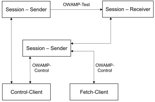
This OWAMP discuss methodology to create an environment to collect IPPM metrics from mesh of Internet paths. OWAMP consist of two protocols: OWAMP – Control and OWAMP – test. The OWAMP Control is used to initiate, start and stop the test sessions, and OWAMP test actually engage itself test data exchanges between the OWAMP servers [49]. The correlation between this methodology and flowgrind is discussed in the section 5.3.

The OWAMP – Control entity involves the session initiation, which basically exchange the source and destination address, port number between the OWAMP servers, and exchange of the testing parameter like test session length, test packet size, and it also discusses regarding the per session encryption and authentication, but these topics are out of scope of this section [49]. OWAMP divides the each entity into a logical model, and each logical model has its own standard definition and functionality. It is shown in the figure 2.1 [49].

Session Sender: The sending terminal in the OWAMP – test session. Session Receiver: The receiving terminal in the OWAMP – test session.

(24)

Server: The node that actually involves in least one test session or more, and returns the test result to the client.

Control – Client: The node that request for the test session with servers, induces start and termination for the test session.

Fetch – Client: The entity that fetch the results from the server for the terminated test session OWAMP protocol is actually an UDP test traffic, which uses TCP connection for the OWAMP Control and UDP connection for the measurement session in the OWAMP test. The discussion regarding the implementation of the OWAMP-Control, Connection Setup and the modes of operation is out of scope for this section.

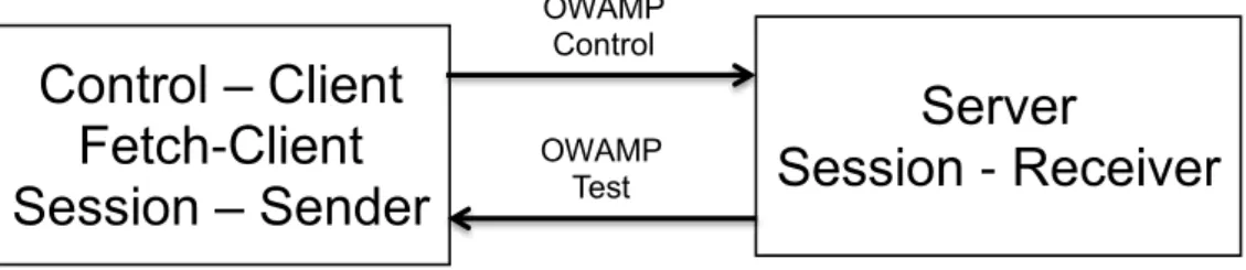
The one way delay measurement is done according to methodology in RFC 2679; the send timestamp is filled in the test data along with the error estimate, error estimate is used to share the information, regarding the clock synchronization with the UTC, using GPS hardware, or by using NTP [49]. The logical model as shown in the figure 2.1 can also be configured as client-server architecture as shown in the figure 2.2 [49].

Session – Sender OWAMP-Test Session – Receiver

Session – Sender

Control-Client Fetch-Client

OWAMP-Control

(25)

2.8 Conclusion

Control – Client

Fetch-Client

Session – Sender

Server

Session - Receiver

OWAMP Control OWAMP

Test

Figure 2.2: One-way active measurement protocol client and server architecture

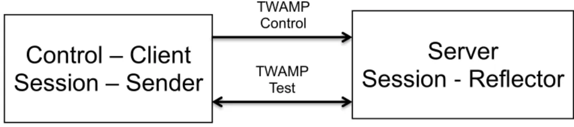
2.7.2 Two-Way Active Measurement Protocol (TWAMP) -RFC 5357

For the two way delay measurement, there is no need for the both source and destination clock to be synchronized with each other. TWAMP implementation uses the methodology and procedure as mentioned in the OWAMP. But in addition to the OWAMP, the destination echo backs the source timestamp back to the source as response packet from the destination [35].

There are few differences between the OWAMP and TWAMP logical model, the role and function of the different logical entities are given as below. The logical model in the client - server architecture is shown in the figure 2.3.

Session-Reflector: The session receiver is called as session reflector, since session reflector has the ability to send back or echo back the packets, which it receives from the source and it doesn’t collect any information regarding the packet from the server.

Server: The TWAMP server is similar to the OWAMP server but the TWAMP server doesn’t have the capability to return the results because the results are not calculated at the server.

Fetch-client: This item doesn’t exist in the TWAMP, since session reflector doesn’t collect any information from the server. So there is no need to fetch information from the server.

The methodology to measures the two delays in TWAMP is similar to the procedure explained in the RFC 2681.

2.8 Conclusion

This chapter explains in detail, regarding the standard procedure maintained in the IETF’s IPPM working group for measuring the one way delay and two delay performance metrics. This gives us the overall picture regarding the one way delay and two way

(26)

Control – Client

Session – Sender

Server

Session - Reflector

TWAMP Control TWAMP

Test

Figure 2.3: Two-way active measurement protocol client and server architecture

delay definition, methodology, errors and uncertainty in the results due to the clock synchronization issues in both source and destination side. The standard methodology to measure the latency as defined by the IETF working group and the latency measurement implementation by the performance metrics are correlated in the upcoming chapters.

(27)

3 Performance tools

With more advancement and increasing level of research in the forms of high speed networks to meet today’s internet there lies a motivation to find genuine and objective benchmarks against the quality of services offered in a network. With the increase in the speed with broadband services, there is always a concern for the end users about the performance of the network.

High speed networking is not the answer in terms of performance for the broad spectrum [32]. The ability of the network to support the transactions that include the transfer of large amount of data and also support multiple and parallel transactions will give an overall picture of large network with heavy load condition and also network performance [3].

A good approach to measure the network performance is to inject test traffic into the network and measure the network performance, and then relate the performance of the test traffic to the performance of the network in carrying the normal payload. In this chapter, the performance tools and their measurement methodology will be discussed in detail.

3.1 ICMP Ping

Most widely used measurement tool isping. The ping is a very simple tool to generate the Internet Control Message Protocol (ICMP) echo request packet, and directs it to destination host. When the packet is sent, the source host will start system clock timer operation. The destination host reverses the ICMP headers and sends back the ICMP echo reply packet to the source. When source receive the ICMP echo reply packet, then the timer is halted and the elapsed time is reported [32].

This indicates that the destination system is connected to the network, and is reachable from the source system. Failure of response from the destination host is not much informative, because it cannot be actually interpreted and that the destination system is not available in the network. Reason for this is that the destination response packet may have been discarded in the network due to the network congestion, and also the network path is not available to the destination. The firewall rules between the source and destination may block the destination response packet from being delivered [32]. The ICMP ping results can give some useful performance metrics information. The elapsed duration for a ping packets response, from the destination to source giving the

(28)

3 Performance tools

depiction of the response time and their standard deviation, suggests the load being experienced on the network path between the source and destination. The increased load in the network will be revealed as increased delay and their standard deviation, since the presence of large router buffers along the network path [32].

The ICMP packets could be discarded by router, if there is buffer overflows in the router. This will result in the increase of the ping loss in the network. The unpredictable high latency and loss within ping packets shows the instability within the network path. Several router architectures use fast switching paths for data transmit, however the Central Processing Unit (CPU) of the router process the ping request and response. So the ping response might be given lesser scheduling priority because router functions represent more critical operation. So in this case, there is a possibility that extended delays will be reported by the ICMP ping [32].

In more details, the typical Transmission Control Protocol (TCP) flow behavior is vulnerable to cluster into bursts of packet transmission. But ping doesn’t need or not having any necessities to echo similar behavior. So the ping can only be used in a primordial way to discover the provisioned capacity of network connectivity [32].

3.2 Thrulay

Thrulay stands for THRUput and deLAY. The feature, which distinguishes the thrulay from the previous performance tools, is that thrulay reports delay information in addition to the throughput metrics. Thrulay measures throughput and round trip time by transmitting a bulk TCP stream over the network. Thrulay also supports UDP protocol in addition to the TCP, but it measures only the one-way delay for UDP packets. In UDP testing, thrulay sends a Poisson stream of very precisely positioned UDP packets [51].

The thrulay is initially developed for the measuring Round Trip Time (RTT) for the FAST TCP, but useful for standard loss – based TCP too [52]. The figure 3.1 shows the Thrulay example output for the bulk Transfer test.

3.3 TTCP and NUTTCP

The Test TCP (TTCP) [13] used to measure goodputs for both TCP and UDP packets. For the UDP packets it also displays packet loss rate. TTCP is client-server architecture, which means it can measure only unidirectional flows from client to the server [13]. The tool NUTTCP is the successor of TTCP, which has several additional features compare to the TTCP. The NUTTCP starts the test between two servers, whereas the test

(29)

3.4 Iperf

phobos2 :~/ thrulay -ng -0.6.2/ src % ./ thrulay 172.16.121.21 -t 10 s

# local window = 425984 B; remote window = 425984 B

# block size = 8192 B

# MTU : 1500 B; MSS : 1448 B; Topology guess : Ethernet / PPP

# MTU = getsockopt ( IP \ _MTU ); MSS = getsockopt ( TCP \ _MAXSEG )

# test duration = 10 s; reporting interval = 1s

#( ID ) begin , s end , s Mb /s RTT , ms : min avg max ( 0) 0.000 1.000 14311.627 0.083 0.285 0.613 ( 0) 1.000 2.000 15691.994 0.142 0.243 0.430 ( 0) 2.000 3.000 15724.855 0.142 0.241 0.433 ( 0) 3.000 4.000 15855.333 0.144 0.239 0.364 ( 0) 4.000 5.000 15777.006 0.151 0.241 0.426 ( 0) 5.000 6.000 15895.364 0.151 0.239 0.368 ( 0) 6.000 7.000 15860.941 0.145 0.239 0.361 ( 0) 7.000 8.000 15791.112 0.151 0.241 0.373 ( 0) 8.000 9.000 15908.691 0.151 0.238 0.426 ( 0) 9.000 10.000 15872.557 0.150 0.240 0.361

#( 0) 0.000 10.000 15668.922 0.083 0.244 0.613

#(**) 0.000 10.000 15668.922 0.083 0.244 0.613

Figure 3.1: Thrulay example output: TCP bulk transfer test

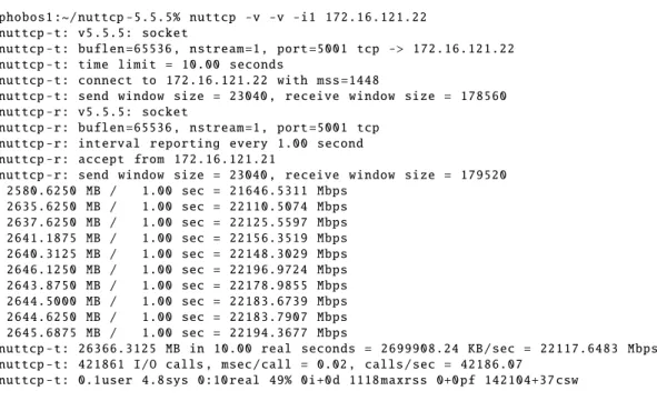
started by NUTTCP client could be from the system. The NUTTCP client submit the test parameters to servers and then servers will establish the data connection between them to perform the measurements [42]. The test results are aggregated and sent back to the NUTTCP client, where it is displayed. The figure 3.2 shows the NUTTCP example output for the bulk Transfer test.

The NUTTCP report the total amount of data sent, average throughput per second, CPU usage in percentage for both source and destination, uses theTCP_INFOsocket option to display the number of retransmission on NUTTCP data connection between the servers, and average RTT measured. NUTTCP also reports the results per interval.

3.4 Iperf

Iperf is relatively simple tool, it is based on the client-server architecture. It is primarily used to measure the goodput. To start the test, the Iperf client connects to the Iperf server and sends the test parameter to the server and then starts the bulk data transfer between client and server. The Iperf measures both the TCP and User Datagram Protocol (UDP) bulk transfer test. By optional in the TCP bulk transfer test, data can optionally be sent in parallel with multiple connections to the same server via multiple threads. The Intermediate tests are displayed at the both Iperf server and client according to the configured time interval testing. The UDP bulk transfer test can also measure the datagram loss rate and delay jitter [33].

But in addition to these advantages, the Iperf also have few demerits. Iperf can only test against one server at a time and unlike NUTTCP does the Iperf does not support third party tests. The Iperf can measure the parameter unidirectional from server to client

(30)

3 Performance tools

phobos1 :~/ nuttcp -5.5.5% nuttcp -v -v -i1 172.16.121.22 nuttcp -t: v5 .5.5: socket

nuttcp -t: buflen =65536 , nstream =1 , port =5001 tcp -> 172.16.121.22 nuttcp -t: time limit = 10.00 seconds

nuttcp -t: connect to 172.16.121.22 with mss =1448

nuttcp -t: send window size = 23040 , receive window size = 178560 nuttcp -r: v5 .5.5: socket

nuttcp -r: buflen =65536 , nstream =1 , port =5001 tcp nuttcp -r: interval reporting every 1.00 second nuttcp -r: accept from 172.16.121.21

nuttcp -r: send window size = 23040 , receive window size = 179520 2580.6250 MB / 1.00 sec = 21646.5311 Mbps

2635.6250 MB / 1.00 sec = 22110.5074 Mbps 2637.6250 MB / 1.00 sec = 22125.5597 Mbps 2641.1875 MB / 1.00 sec = 22156.3519 Mbps 2640.3125 MB / 1.00 sec = 22148.3029 Mbps 2646.1250 MB / 1.00 sec = 22196.9724 Mbps 2643.8750 MB / 1.00 sec = 22178.9855 Mbps 2644.5000 MB / 1.00 sec = 22183.6739 Mbps 2644.6250 MB / 1.00 sec = 22183.7907 Mbps 2645.6875 MB / 1.00 sec = 22194.3677 Mbps

nuttcp -t: 26366.3125 MB in 10.00 real seconds = 2699908.24 KB / sec = 22117.6483 Mbps nuttcp -t: 421861 I/O calls , msec / call = 0.02 , calls / sec = 42186.07

nuttcp -t: 0.1 user 4.8 sys 0:10 real 49% 0i +0 d 1118 maxrss 0+0 pf 142104+37 csw

nuttcp -r: 26366.3125 MB in 10.00 real seconds = 2699623.97 KB / sec = 22115.3196 Mbps nuttcp -r: 421864 I/O calls , msec / call = 0.02 , calls / sec = 42181.92

nuttcp -r: 0.0 user 9.9 sys 0:10 real 99% 0i +0 d 96 maxrss 0+16 pf 4+105 csw

Figure 3.2: NUTTCP example output: TCP bulk transfer test

and it doesn’t support bidirectional TCP and UDP goodput. In order to simulate the bidirectional TCP connection, the two unidirectional connections are used in the parallel. The figure 3.3 shows the Iperf example output for the bulk Transfer test.

3.5 Netperf

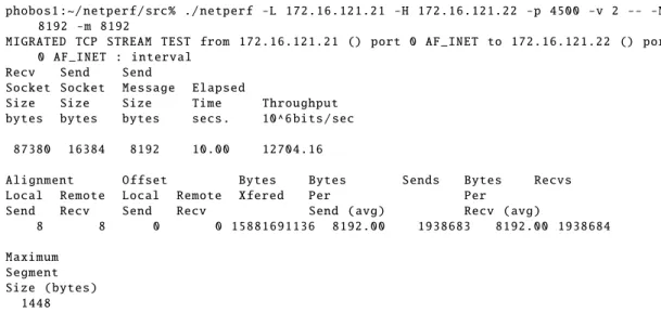
Netperf is also a client-server based measurement tool, similar to Iperf and doesn’t support the third party test. It can also only test against one single server at a time. Netperf is able to use Unix Domain sockets and the data link provider interface and supports Stream Control Transmission Protocol (SCTP) in addition to the TCP and UDP protocol. It is developed by Hewlett-Packard. Netperf provides different testing for the different protocol. TCP_Steam is the most basic test for the TCP protocol, which used to measure unidirectional TCP good put for the bulk data transfers. The figure 3.4 shows the Netperf example output for the bulk Transfer test.

Netperf also supports the request-response test called as TCP_RR in which Netperf measure the transaction rate [41]. In addition to these tests, Netperf is used to measure TCP connection establishment and also the closure. If these tests are combined with the request-response (TCP_RR), the resulting network load is not equivalent to the Hypertext

(31)

3.5 Netperf

phobos1 :~/ iperf / src % iperf3 -c 172.16.121.22 -B 172.16.121.21 -l 8192 -i 1 Connecting to host 172.16.121.22 , port 5201

[ 4] local 172.16.121.21 port 36904 connected to 172.16.121.22 port 5201 [ ID ] Interval Transfer Bandwidth Retr

[ 4] 0.00 -1.00 sec 1.91 GBytes 16.4 Gbits / sec 0 [ 4] 1.00 -2.00 sec 1.91 GBytes 16.4 Gbits / sec 0 [ 4] 2.00 -3.00 sec 1.91 GBytes 16.4 Gbits / sec 0 [ 4] 3.00 -4.00 sec 1.92 GBytes 16.5 Gbits / sec 0 [ 4] 4.00 -5.00 sec 1.91 GBytes 16.4 Gbits / sec 0 [ 4] 5.00 -6.00 sec 1.92 GBytes 16.5 Gbits / sec 0 [ 4] 6.00 -7.00 sec 1.92 GBytes 16.5 Gbits / sec 0 [ 4] 7.00 -8.00 sec 1.92 GBytes 16.5 Gbits / sec 0 [ 4] 8.00 -9.00 sec 1.92 GBytes 16.5 Gbits / sec 0 [ 4] 9.00 -10.00 sec 1.92 GBytes 16.5 Gbits / sec 0

-[ ID ] Interval Transfer Bandwidth Retr

[ 4] 0.00 -10.00 sec 19.2 GBytes 16.5 Gbits / sec 0 sender [ 4] 0.00 -10.00 sec 19.2 GBytes 16.5 Gbits / sec receiver iperf Done .

Figure 3.3: Iperf example output: TCP bulk transfer test

Transfer Protocol (HTTP) traffic. The results in such scenarios could be considered as basic traffic generation test. The Netperf can measure the overall CPU utilization on both source and destination host as well as the service demand, which is the number of CPU time spent per measurement unit, for example, the CPU time needed for a single transaction for the request- response tests.

phobos1 :~/ netperf / src % ./ netperf -L 172.16.121.21 -H 172.16.121.22 -p 4500 -v 2 -- -M 8192 -m 8192

MIGRATED TCP STREAM TEST from 172.16.121.21 () port 0 AF_INET to 172.16.121.22 () port 0 AF_INET : interval

Recv Send Send

Socket Socket Message Elapsed

Size Size Size Time Throughput bytes bytes bytes secs . 10^6 bits / sec

87380 16384 8192 10.00 12704.16

Alignment Offset Bytes Bytes Sends Bytes Recvs Local Remote Local Remote Xfered Per Per

Send Recv Send Recv Send ( avg ) Recv ( avg )

8 8 0 0 15881691136 8192.00 1938683 8192.00 1938684 Maximum

Segment Size ( bytes )

1448

(32)

3 Performance tools

3.6 Drawback of existing performance tools

The main drawback of previously discussed performance measurement tools is their client-server architecture, which makes the transmission of test data through the network along multiple paths in parallel difficult. To test the multiple paths, the clients need to execute in parallel on different nodes and have to run the server multiple times as well. Using the client – server architecture based tools to set up testing framework that involves multiple clients in a monotonous task. As well as these scenarios lead to the synchronization problems as well. For example, even if the two clients start the testing at the same time, there might be a chance that one client is still exchanging the testing parameters with its server, while the other clients have already begun the actual data testing with the server. The consequence of this lack of synchronization leads to the inaccurate results in the testing [62].

The bidirectional protocols like TCP can send the data in the both directions at the same time. But unfortunately all these tools support only unidirectional data transfer that means these tools can only generate unidirectional traffic on an individual test connection. Trying to simulate the bidirectional loads through the use of two parallel unidirectional test connections doesn’t represent the accurate model of true bidirectional test connections [62].

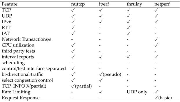
Table 3.1: Performance measurement tools feature matrix

Feature nuttcp iperf thrulay netperf

TCP X X X X

UDP X X X X

IPv6 X X X X

RTT X - X

-IAT X - X

-Network Transactions/s - - - X

CPU utilization X - - X

third party tests X - -

-interval reports X X X X

scheduling - - -

-control/test interface separated X - -

-bi-directional traffic X X(pseudo) -

-select congestion control X X -

-TCP_INFO X(partial) X(partial) - -

-Rate Limiting - X UDP only X

(33)

3.7 Conclusion

This chapter discuss in details regarding the present performance measurement tools and the comparison regarding their features is shown in the table 3.1. All the tools discussed in this chapter couldn’t generate the realistic internet traffic. This is considered as the one of the disadvantage of these tools. The details regarding the traffic generation is discussed in the next chapter.

(34)

(35)

4 Traffic Generation model

This chapter gives an overview regarding the stochastic traffic generation in the flowgrind. Additionally this section gives the mathematical model behind the stochastic traffic generation in basic. The section gives the details regarding the traffic model and scenarios generated by traffic generation.

4.1 Introduction to Traffic Generation model

Developing a traffic generation, for example a pragmatic internet is a challenge task. In general there are two primitive methods to generate manifold internet traffic. A basic and easy approach is to record cluster of traffic, and subsequently re-run them. This approach is calledtraffic replay[31]. Another approach to generate pragmatic traffic by using the stochastic process, this method is called as thestochastic traffic generation[47]. Both the methods, has its own advantages and disadvantages, because of their way, in which these approaches are developed. The traffic replay method is more pragmatic, since trace record is the combination of the data streams and the traffic attributes and it reproduces the trace records with the same traffic attributes [31]. Despite the easy implementation of the traffic replay, it has its own demerits because traffic replay considers the trace records as the black box and it is difficult to change the traffic to test different test scenarios [47]. And other demerits of the traffic replay approach are that it requires additional procedure and resources to record the traces, process and store them.

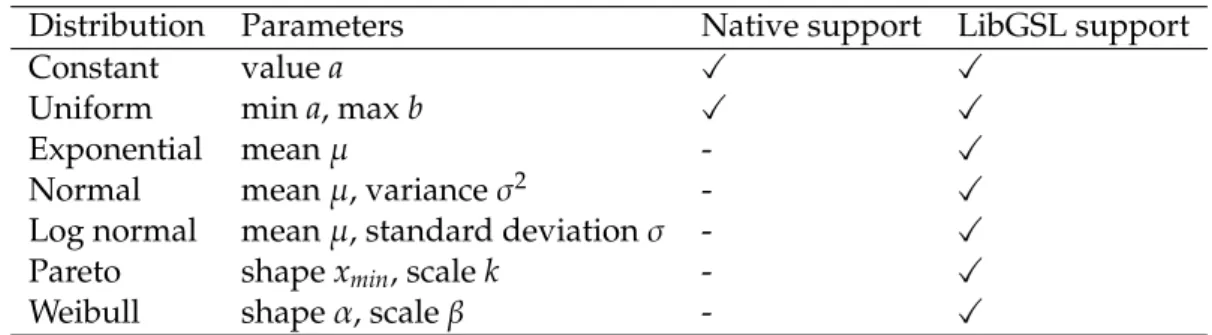
In contrast, the stochastic traffic generation generates the traffic based on the mathematical model for different traffic and workload characteristics. One of the useful features in the stochastic model is that the parameters can be extracted from quantitative analysis. This feature in the stochastic traffic generation compels it to do experiment protocols and evaluate them, before actually doing the implementation work for the protocols [47]. Another disadvantage of the traffic replay method is that difference between the traffic noise and the payload in the trace records requires additional information for boundaries in the data set [47]. The whole trace records are needed to store in traffic replay, but in contrast to it, the stochastic traffic generation, requires to store only the parameter to generate the stochastic traffic generation and random state number. The flowgrind stochastic traffic generation has been discussed in this section 5.8

(36)

4 Traffic Generation model

4.2 Mathematical Background

The branches of mathematics namely probability theory and statistics are the bases for the stochastic. The probability distribution plays a vital role in the probability theory. The random variable is the basis for the probability distribution. For each experiment, the random element allocates a value to each possible result [10].

For instance, let us take a scenario of random variable Y for a coin flipping, which could be like this

Y= (

0, if head, 1, if tail.

In the following procedure, let us add the probability to the value of possible results which leads to the probability distribution. In our experiment of coin flipping, the value of the probability for the head and tail should be 0.5. But let us consider that the coin is biased or manipulated and the final results could be possible as.

Y= (

1/3, 0,if head, 2/3, 1,if tail.

The given resultant value is called as the discrete probability distribution. If there is a finite set in the probability distribution, where the sum of the set is 1, then that probability distribution is considered as the discrete [10].

The continuous probability distribution in contrast to discrete probability distribution has a continuous random element Y with a probability density function f(Y):

Pr [a≤_Y≤_b_]=Rb a f(y)dy

A probability density function for the random element Y plots the corresponding possibility for this element to exist at a given point in a set. The integral of random element density result in the probability for the random element within the given set. This statement implicit the probability of single value is zero, for instance for the z value, the probabilityz≤_Y≤_z_{is zero. This is because the integral value with same upper and}

(37)

4.3 Traffic model

This section contains information regarding the cdma 2000 Evaluation methodology theoretical mode [1] for the internet traffic, mainly for the HTTP protocol.

The reference to the technical document, which describes the traffic model for the different network traffic, is designed on the concepts of empirical analysis of cellular network traffic [1]. Although this model is recommended for the traffic model for the 3G hardware evaluation, the basic traffic model for the Hypertext Transfer Protocol (HTTP) traffic can be adopted for other protocol evaluation as well. From the technical document [1], the HTTP traffic has six components. The main object size (SM), the embedded object size (SE), the number of embedded objects per page (Nd), the reading time (Dpc), the initial reading time (Dipc) and the parsing time (Tp) taken from the technical document [1]. The HTTP request size is fixed for 350 byte in this model.

The requirement for the traffic model is simple. The implementation of passing parameter should be simple and at the same time, it should be able to emulate protocol, for instance like the HTTP traffic and Teletype Network (TELNET). Since the cdma 2000 evaluation methodology uses more parameter, it should be designed with less parameter. The chosen parameter for the traffic models are given below.

Request size: This size represents the single request block. For example, in a single website the block represent the smallest unit of the transferred data. It is denotes asSq Response size: This size represents the single response block. If the response block is greater than zero, then with each request block, a response block is requested according to the response size. It is denoted asSp

Interdeparture time: The time gap between two request size block can be used for the two purposes, one is for the rate limit request, in the case of reading a website in HTTP protocol and another one is to achieve the wait time, in the case of waiting for the user input in the TELNET protocol. It also represents the Interdepature Gap. It is denoted as Tg

The parameter is used in the cdma 2000 Evaluation methodology. For instance, the parsing time (Tp), reading time (Dpc), initial reading time (Dipc) can be managed by using only the Interdepature timeTg

4.4 Traffic generation use cases

This section generally list the possible and general use cases possible through the Traffic model, this gives a general overview picture of the use cases used in the actual measurement scenario and discussed in detail in result section 7.3

(38)

4 Traffic Generation model

Rate limited flows: This scenario is used in generation use case for rate timed media streaming and sender limited flows. The interdeparture Tg is added between two request block. The sending rate can be expressed asbyte/s, or in theblock/sformat. The interpacket gap can be computed from specifying the target sending rate.

Interdepature timeTg[s]= block size

bytes write rate

" bytes

s #

The burst behavior in the Transmission Control Protocol (TCP) can be affected by changing the written or request block size from the above formula. It always writes the whole data into socket at a single shot, this leads to a smooth data transfer, whether the block size is of greater or smaller value. This transfer characterizes could be made less deterministic, by applying the normal distribution for the interpacket gap.

Bulk transfer flow:The bulk transfer flow can be modelled using the traffic generation model with constant distribution for the request sizeSq, and both respond sizeSpand interdeparture timeTgare set to zero. For instance, File Transfer Protocol (FTP) the file transfer protocol could be emulated by the bulk transfer flow.

Request-Response flow: The common flow for many existing traffic model is the request-response flow. The simple concept of the request and response flow is that a sender sends a block (the request size block) and receiver responds back to the sender with another block(the response block). This communication model can be emulated by changing the request sizeSqand response blockSp. And the interdeparture timeTgwith different values, can emulate different protocols like HTTP, TELNET and Simple Mail Transfer Protocol (SMTP).

4.5 Conclusion

This chapter gives the over views of the fundamental and basic procedure to implement the generic traffic model and in addition it also explains actual implementation of the Stochastic model in the flowgrind. The practical use of different use cases for the measurement results are discussed in this section and these are directly applied to the test procedure. In order to understand the flowgrind traffic generation in the section 5.8 and the test procedure in the section 7.3 this chapter is useful.

(39)

5 Flowgrind

The objective of the thesis is to develop the latency measurement module using the existing and suitable performance tools. The chapter 2 discusses regarding the methodology of latency measurement procedure, and chapter 4 discusses regarding the generation of diverse traffic to emulate the workload condition. This chapter gives details regarding performance measurement toolflowgrind, which supports the traffic generation and also discuss the advantage of implementation of the latency measurement module in the flowgrind.

5.1 Introduction to flowgrind

Flowgrind supports distributed architecture and performs measurements against an arbitrary number of end-points simultaneously. One or more test connections are called as “flows” in the flowgrind. These flows could be scheduled to run consecutively, interleaved and fully synchronized. Each flow could be assigned with a duration and an initial delay. Actual test connection starts after the initial delay. In addition to this, each flow have its own testing parameters, which are called as“flow options”, which can be set individually for each direction [62].

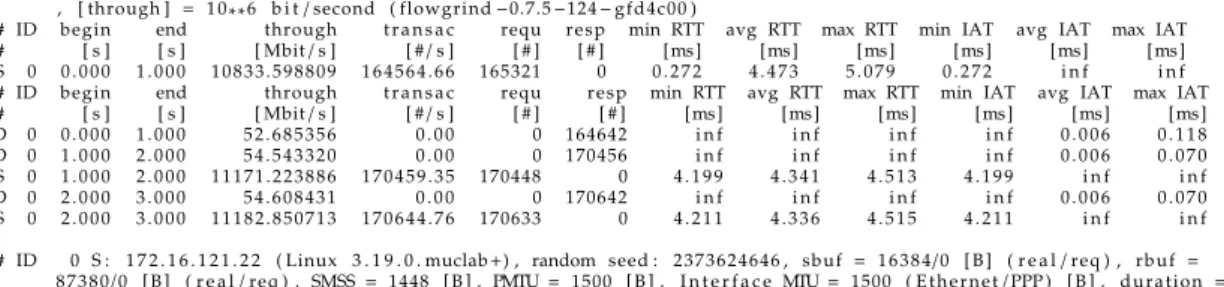
The flowgrind continuously outputs the data according to the flow option interval timing, which can be configured individually with millisecond precision. This provides not only very fine grained reporting, but also coarse intervals like reporting in seconds and minutes. Flowgrind have an extra feature to report regarding the Transmission Control Protocol (TCP)-specific performance metrics. These metrics are obtained from the linux kernel using theTCP_INFOsocket option. Similar to all other performance metrics, TCP-specific metrics are collected by the flowgrind and sample at the end of reporting time interval specified by its flow option. The figure 5.1 and 5.2 shows the basic flowgrind output

5.2 History

The flowgrind performance tool is loosely related to thrulay tool developed by Stanislav Shalunow [50] which has been developed back 2005. These inspired researchers [62] developed a performance measurement tool specialized for evaluation of TCP/IP stack and measuring the performance metrics. The earlier version of the flowgrind aimed to

(40)

5 Flowgrind

phobos2 : ~/flowgrind% ./flowgrind −_{c through , t r a n s a c , i n t e r v a l , i a t , b l o c k s} −_{i 1} −_{T s=3} −_{A s} −_{H s}_{=1 7 2 . 1 6 . 1 2 1 . 2 2 , d} =1 7 2 . 1 6 . 1 2 1 . 2 1

# Date : 2015−₀₄−₂₆−_{21:42:25 , c o n t r o l l i n g h o s t} ₌_{phobos2 . mgmt . muclab , number o f flows} ₌ _{1 , r e p o r t i n g i n t e r v a l} ₌ _{1 . 0 0 s} , [ through ] = 1 0 **6 b i t/second ( flowgrind−_0.7.5−₁₂₄−_{gfd4c00 )}

# ID begin end through t r a n s a c requ r e s p min RTT avg RTT max RTT min IAT avg IAT max IAT # [ s ] [ s ] [ Mbit/s ] [ #/s ] [ # ] [ # ] [ms] [ms] [ms] [ms] [ms] [ms] S 0 0 . 0 0 0 1 . 0 0 0 1 0 8 3 3 . 5 9 8 8 0 9 1 6 4 5 6 4 . 6 6 165321 0 0 . 2 7 2 4 . 4 7 3 5 . 0 7 9 0 . 2 7 2 i n f i n f # ID begin end through t r a n s a c requ r e s p min RTT avg RTT max RTT min IAT avg IAT max IAT # [ s ] [ s ] [ Mbit/s ] [ #/s ] [ # ] [ # ] [ms] [ms] [ms] [ms] [ms] [ms] D 0 0 . 0 0 0 1 . 0 0 0 5 2 . 6 8 5 3 5 6 0 . 0 0 0 164642 i n f i n f i n f i n f 0 . 0 0 6 0 . 1 1 8 D 0 1 . 0 0 0 2 . 0 0 0 5 4 . 5 4 3 3 2 0 0 . 0 0 0 170456 i n f i n f i n f i n f 0 . 0 0 6 0 . 0 7 0 S 0 1 . 0 0 0 2 . 0 0 0 1 1 1 7 1 . 2 2 3 8 8 6 1 7 0 4 5 9 . 3 5 170448 0 4 . 1 9 9 4 . 3 4 1 4 . 5 1 3 4 . 1 9 9 i n f i n f D 0 2 . 0 0 0 3 . 0 0 0 5 4 . 6 0 8 4 3 1 0 . 0 0 0 170642 i n f i n f i n f i n f 0 . 0 0 6 0 . 0 7 0 S 0 2 . 0 0 0 3 . 0 0 0 1 1 1 8 2 . 8 5 0 7 1 3 1 7 0 6 4 4 . 7 6 170633 0 4 . 2 1 1 4 . 3 3 6 4 . 5 1 5 4 . 2 1 1 i n f i n f # ID 0 S : 1 7 2 . 1 6 . 1 2 1 . 2 2 ( Linux 3 . 1 9 . 0 . muclab+) , random seed : 2 3 7 3 6 2 4 6 4 6 , sbuf = 1 6 3 8 4/0 [ B ] ( r e a l/req ) , r b u f =

8 7 3 8 0/0 [ B ] ( r e a l/req ) , SMSS= 1448 [ B ] , PMTU= 1500 [ B ] , I n t e r f a c e MTU=1500 ( E t h e r n e t/PPP ) [ B ] , d u r a t i o n = 3 . 0 0 0/3 . 0 0 0 [ s ] ( r e a l/req ) , through = 1 1 0 6 2 . 5 4 4 4 4 8/5 3 . 9 3 7 9 3 0 [ Mbit/s ] ( out/i n ) , t r a n s a c t i o n s/s= 1 6 8 5 5 6 . 0 3 [ # ] , r e q u e s t b l o c k s = 5 0 6 4 0 2/0 [ # ] ( out/i n ) , response b l o c k s= 0/5 0 5 6 6 7 [ # ] ( out/i n ) , RTT= 0 . 2 7 2/4 . 3 8 2/5 . 0 7 9 [ms] ( min/avg/max )

# ID 0 D: 1 7 2 . 1 6 . 1 2 1 . 2 1 ( Linux 3 . 1 9 . 0 . muclab+) , random seed : 2 3 7 3 6 2 4 6 4 6 , sbuf = 1 6 3 8 4/0 [ B ] ( r e a l/req ) , r b u f = 8 7 3 8 0/0 [ B ] ( r e a l/req ) , SMSS= 1448 [ B ] , PMTU= 1500 [ B ] , I n t e r f a c e MTU=1500 ( E t h e r n e t/PPP ) [ B ] , through = 5 3 . 9 4 5 6 8 1/1 1 0 4 8 . 0 7 5 4 6 3 [ Mbit/s ] ( out/i n ) , r e q u e s t b l o c k s = 0/5 0 5 7 4 0 [ # ] ( out/i n ) , response b l o c k s = 5 0 5 7 4 0/0 [ # ] ( out/i n ) , IAT= 0 . 0 0 3/0 . 0 0 6/0 . 1 1 8 [ms] ( min/avg/max ) , delay = 0 . 1 9 2/4 . 2 6 4/4 . 9 4 4 [ms] ( min/avg/max )

Figure 5.1: Flowgrind example output: Measurement without kernel output phobos2 : ~/flowgrind% ./flowgrind −_{c through , k e r n e l ,} −_{i 1} −_{T s}₌₃−_{A s} −_{H s}₌_{1 7 2 . 1 6 . 1 2 1 . 2 2 , d=}_{1 7 2 . 1 6 . 1 2 1 . 2 1}

# Date : 2015−₀₄−₂₆−_{21:46:29 , c o n t r o l l i n g h o s t} ₌_{phobos2 . mgmt . muclab , number o f flows} ₌ _{1 , r e p o r t i n g i n t e r v a l} ₌ _{1 . 0 0 s} , [ through ] = 1 0 **6 b i t/second ( flowgrind−_0.7.5−₁₂₄−_{gfd4c00 )}

# ID through min RTT avg RTT max RTT cwnd s s t h uack sack l o s t r e t r t r e t f a c k r e o r bkof r t t r t t v a r r t o ca s t a t e smss pmtu

# [ Mbit/s ] [ms] [ms] [ms] [ # ] [ # ] [ # ] [ # ] [ # ] [ # ] [ # ] [ # ] [ # ] [ # ] [ms] [ ms] [ms] [ B ] [ B ]

S 0 1 0 9 6 7 . 5 4 0 8 7 6 0 . 2 2 0 4 . 3 9 4 4 . 9 8 2 204 171 136 0 0 0 0 0 3 0 0 . 1 0 . 0 2 0 1 . 0 open 1448 1500

S 0 1 1 1 6 0 . 9 9 6 1 4 9 4 . 1 8 0 4 . 3 2 6 4 . 4 9 9 204 171 34 0 0 0 0 0 3 0 0 . 1 0 . 0 2 0 1 . 0 open 1448 1500

D 0 5 3 . 3 3 6 9 5 4 i n f i n f i n f 10 17 1 0 0 0 0 0 3 0 0 . 1 0 . 0 2 0 1 . 0 open 1448 1500

D 0 5 4 . 4 9 9 7 8 9 i n f i n f i n f 10 17 1 0 0 0 0 0 3 0 0 . 1 0 . 0 2 0 1 . 0 open 1448 1500

S 0 1 1 1 7 4 . 3 0 7 9 3 0 4 . 1 5 3 4 . 3 2 0 4 . 4 9 9 204 171 9 0 0 0 0 0 3 0 0 . 1 0 . 0 2 0 1 . 0 open 1448 1500

D 0 5 4 . 5 7 3 2 2 2 i n f i n f i n f 10 17 1 0 0 0 0 0 3 0 0 . 1 0 . 0 2 0 1 . 0 open 1448 1500

# ID 0 S : 1 7 2 . 1 6 . 1 2 1 . 2 2 ( Linux 3 . 1 9 . 0 . muclab+) , random seed : 3 8 2 6 2 8 9 7 5 9 , sbuf = 1 6 3 8 4/0 [ B ] ( r e a l/req ) , r b u f = 8 7 3 8 0/0 [ B ] ( r e a l/req ) , SMSS= 1448 [ B ] , PMTU= 1500 [ B ] , I n t e r f a c e MTU=1500 ( E t h e r n e t/PPP ) [ B ] , d u r a t i o n = 3 . 0 0 0/3 . 0 0 0 [ s ] ( r e a l/req ) , through = 1 1 1 0 0 . 9 5 0 7 1 9/5 4 . 1 2 5 0 3 5 [ Mbit/s ] ( out/i n ) , t r a n s a c t i o n s/s= 1 6 9 1 4 0 . 7 3 [ # ] , r e q u e s t b l o c k s = 5 0 8 1 6 5/0 [ # ] ( out/i n ) , response b l o c k s= 0/5 0 7 4 2 6 [ # ] ( out/i n ) , RTT= 0 . 2 2 0/4 . 3 4 6/4 . 9 8 2 [ms] ( min/avg/max )

# ID 0 D: 1 7 2 . 1 6 . 1 2 1 . 2 1 ( Linux 3 . 1 9 . 0 . muclab+) , random seed : 3 8 2 6 2 8 9 7 5 9 , sbuf = 1 6 3 8 4/0 [ B ] ( r e a l/req ) , r b u f = 8 7 3 8 0/0 [ B ] ( r e a l/req ) , SMSS= 1448 [ B ] , PMTU= 1500 [ B ] , I n t e r f a c e MTU=1500 ( E t h e r n e t/PPP ) [ B ] , through = 5 4 . 1 3 6 6 2 0/1 1 0 8 7 . 1 7 9 7 7 0 [ Mbit/s ] ( out/i n ) , r e q u e s t b l o c k s = 0/5 0 7 5 3 0 [ # ] ( out/i n ) , response b l o c k s = 5 0 7 5 3 0/0 [ # ] ( out/i n ) , IAT= 0 . 0 0 3/0 . 0 0 6/0 . 0 8 5 [ms] ( min/avg/max ) , delay = 0 . 0 2 1/4 . 2 2 4/4 . 8 4 8 [ms] ( min/avg/max )

Figure 5.2: Flowgrind example output: Measurement with kernel output

evaluate the TCP in Wireless Mesh Network (WMN), but it was found out that, at that time there was no appropriate tool available for evaluating the TCP for the WMN. So the flowgrind performance tool was developed based on the inspiration and concepts of the thrulay. In the later release, distributed architecture feature was added to the flowgrind to overreach the distributed architecture issue related with the WMNs. Now the flowgrind is a completely independent performance tool, which has improved a lot when compared to the thrulay performance metrics. Unlike thrulay measure, it is used to measure both the bulk traffic, request-respone test, show the TCP-specific information,

(41)

5.3 Flowgrind architecture

latency measurement. Next logical steps towards the flowgrind is to improve the performance and stability in the tool [62].

5.3 Flowgrind architecture

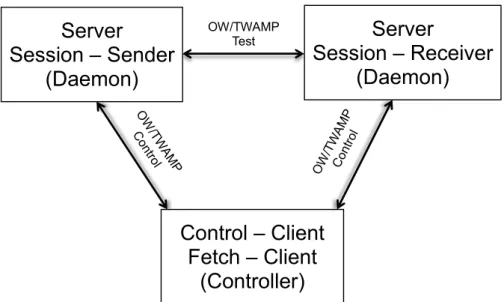
As mentioned earlier, flowgrind supports distributed architecture. This is because the flowgrind by itself is splitted into two parts, the flowgrind daemon (flowgrind) and flowgrind controller. The flowgrind controller doesn’t take part in actual testing and measurement. It is rather used to pass the flow options and flow testing parameter to daemons which are running between the two servers and then these daemons will actually start the testing and measurement process. The performance metrics are sampled by daemons running on the servers. The controller will contact the daemons at the end of every reporting interval. Then the daemons will send back the collected performance metrics data to the controller, and controller displays the results. So the controller doesn’t need to be a part of the tested network. So it is possible to conduct testing between arbitrary servers running flowgrind daemons [62]. So the flowgrind architecture can be correlated with One-way Active Measurement Protocol (OWAMP) in the subsection 2.7.1 and with Two-way Active Measurement Protocol (TWAMP) in subsection 2.7.2 and the logical model for the flowgrind architecture can be drawn as shown in the figure 5.3 based on the logical model discuss in these subsection.

Master s Thesis Evaluation and implementation of a network performance measurement tool for analyzing network performance under heavy workloads

Master’s Thesis

Evaluation and implementation of a

network performance measurement tool

for analyzing network performance under

heavy workloads

Kuralamudhan Ramakrishnan

Hamburg, 04 May 2015

Declaration of Originality

Acknowledgment

Abstract

Contents

1 Introduction

1.1 Motivation

1.2 Objective

1.3 Approach

1.4 Overview

2 Standardization of performance

2.1 IETF

2.2 BMWG

2.3 IPPM

2.4 Bulk Transport Capacity (BTC) – RFC 3148

2.5 One way delay

2.6 Two way delay

2.7 Measurement protocol

Control – Client

Fetch-Client

Session – Sender

Server

Session - Receiver

2.8 Conclusion

Control – Client

Session – Sender

Server

Session - Reflector

3 Performance tools

3.1 ICMP Ping

3.2 Thrulay

3.3 TTCP and NUTTCP

3.4 Iperf

3.5 Netperf

3.6 Drawback of existing performance tools

3.7 Conclusion

4 Traffic Generation model

4.1 Introduction to Traffic Generation model

4.2 Mathematical Background

4.3 Traffic model

4.4 Traffic generation use cases

4.5 Conclusion

5 Flowgrind

5.1 Introduction to flowgrind

5.2 History

5.3 Flowgrind architecture

Control – Client

Fetch – Client

(Controller)

Server

Session – Sender

(Daemon)

Server

Session – Receiver

(Daemon)