Deutsches Institut für Wirtschaftsforschung
www.diw.de
Joachim R. Frick
•Markus M. Grabka
•Olaf Groh-Samberg
D
The Impact of Home Production on
Economic Inequality in Germany
1
59
SOEPpapers
on Multidisciplinary Panel Data Research
SOEPpapers on Multidisciplinary Panel Data Research at DIW Berlin
This series presents research findings based either directly on data from the German Socio-Economic Panel Study (SOEP) or using SOEP data as part of an internationally comparable data set (e.g. CNEF, ECHP, LIS, LWS, CHER/PACO). SOEP is a truly multidisciplinary household panel study covering a wide range of social and behavioral sciences: economics, sociology, psychology, survey methodology, econometrics and applied statistics, educational science, political science, public health, behavioral genetics, demography, geography, and sport science.
The decision to publish a submission in SOEPpapers is made by a board of editors chosen by the DIW Berlin to represent the wide range of disciplines covered by SOEP. There is no external referee process and papers are either accepted or rejected without revision. Papers appear in this series as works in progress and may also appear elsewhere. They often represent preliminary studies and are circulated to encourage discussion. Citation of such a paper should account for its provisional character. A revised version may be requested from the author directly.
Any opinions expressed in this series are those of the author(s) and not those of DIW Berlin. Research disseminated by DIW Berlin may include views on public policy issues, but the institute itself takes no institutional policy positions.
The SOEPpapers are available at
http://www.diw.de/soeppapers
Editors:
Georg Meran (Dean DIW Graduate Center) Gert G. Wagner (Social Sciences)
Joachim R. Frick (Empirical Economics) Jürgen Schupp (Sociology)
Conchita D’Ambrosio (Public Economics)
Christoph Breuer (Sport Science, DIW Research Professor) Anita I. Drever (Geography)
Elke Holst (Gender Studies)
Frieder R. Lang (Psychology, DIW Research Professor) Jörg-Peter Schräpler (Survey Methodology)
C. Katharina Spieß (Educational Science) Martin Spieß (Survey Methodology)
Alan S. Zuckerman (Political Science, DIW Research Professor)
ISSN: 1864-6689 (online)
German Socio-Economic Panel Study (SOEP) DIW Berlin
Mohrenstrasse 58 10117 Berlin, Germany
The Impact of Home Production
on Economic Inequality in Germany
by
Joachim R. Frick*, Markus M. Grabka, Olaf Groh-Samberg
Abstract
Using representative income and time use-data from the German Socio-Economic Panel (SOEP), we estimate non-monetary income advantages arising from home production and analyse their impact on economic inequality. As an alternative to existing measures, we pro-pose a predicted wage approach based on a bias-adjusted measure of hours spent on home production. Sensitivity analyses comparing results obtained from different approaches provide indications of methodological effects arising from the choice of method. Although the sub-stantive notion of reduced inequality is stable, the degree of variation in our findings under-scores the need for a harmonized approach in cross-nationally comparative research.
Keywords: Home Production, Non-Cash Incomes, Economic Inequality, Well-being, SOEP JEL-Codes: D31, D13, I32
Berlin, February 2009
* Corresponding author:
PD Dr. Joachim R. Frick, [email protected] SOEP at DIW Berlin, TU Berlin, IZA Bonn Mohrenstrasse 58, 10117 Berlin, Germany phone: +49-30-89789-279, Fax: +49-30-89789-109
Dr. Markus M. Grabka, [email protected]
SOEP at DIW Berlin
Dr. Olaf Groh-Samberg, [email protected] SOEP at DIW Berlin
Financial support by the European Commission in the context of the research project “Accurate Income Meas-urement for the Assessment of Public Policies” (AIM-AP) 6th Framework Programme, 2006-2009 (Contract Nr. CIT5-CT-2005-028412) is gratefully acknowledged.
Contents
1 Introduction ... 1
2 Measuring Home Production and its Distributional Impact – Literature Review ... 3
3 Deriving a Monetary Value of Home Production Based on Time Use Data ... 10
4 Empirical Results: the Impact of Home Production on Income Inequality... 16
4.1 Population Shares of Beneficiaries... 16
4.2 Income Advantages from Home Production ... 17
4.3 Impact on Income Distribution and Poverty... 19
4.4 Decomposition of Inequality and Poverty by Socio-Economic Structure... 20
5 Conclusion ... 22
6 References... 24
List of Figures & Tables
Table 1: Previous Studies on the Distributional Effect of Home Production ... 26
Table 2: Home Production Activities by Selected Household Characteristics ... 27
Table 3: Home Production by Selected Individual Characteristics... 28
Table 4: Regression of Gross Log Hourly Wages... 29
Table 5: Beneficiaries from Home Production Activities by Income Quintile... 30
Table 6: Income Advantages from Home Production... 31
Table 7: Inequality and Home Production... 32
Figure 1: Lorenz Curves: Baseline Income vs. Extended Income ... 33
Table 8: Inequality Decomposition and Home Production ... 34
Table 9: Poverty Decomposition and Home Production... 35
1 Introduction
1
1
Introduction
Like other types of private in-kind income, such as imputed rent for owner-occupied housing and fringe benefits, home production improves household welfare without being reflected in the household’s cash flow, either in disposable household income or in labor income (see Smeeding and Weinberg 2001). In distributional analyses, the omission of private in-kind incomes may lead to substantially biased results on economic inequality and poverty. Consid-ering income from home production appears to be particularly important in a cross-national perspective, e.g., when comparing countries that differ with respect to the existence of subsis-tence economies or of gender divisions of labor in home production (see Canberra Group 2001).
The aim of this paper is to quantify the value of non-cash income derived from “home production” as well as to analyze its impact on income inequality and poverty in Germany. Extending the scope of home production to include housework, errands, and private care for children and elderly household members, adds a significant share of the overall population as potential beneficiaries of such fictitious income. Estimates for Germany, based on a national time budget survey conducted in 2001/02 among persons aged 10 and over, show that the time spent in unpaid work amounts to as much as 25 hours per normal week, whereas the average number of hours spent in paid work amounts to 17 hours only (BMFSFJ 2003). These figures, of course, vary substantially by sex and age. Roughly estimated, the total time spent on unpaid work equals the amount of time spent for paid work in OECD countries, with the bulk of this amount being provided by women (e.g., Swiebel 1999; OECD 1995). Given that the time spent in home production activities is usually estimated on a lower “wage rate” than paid work, the monetary value of unpaid work in private households typically ranges between
1 Introduction
thirty to fifty percent of GDP (Chadeau 1992; OECD 2006: 113). Thus, despite all the meth-odological and practical problems in deriving a monetary value for household production, one must assume that individuals do draw utility from these activities, which make a significant contribution to their economic wellbeing.
This paper proposes a new “predicted wage” measure for valuing home production and provides first evidence on the distributional impact of home production activities for Germany. Like most of the previous literature on home production, we employ time-use data to estimate the extent and the monetary value of home production, which we do by multiply-ing the (adjusted) number of hours spent in home production by a fictitious hourly wage. The data come from the 2002 wave of the German Socio-Economic Panel (SOEP), a representa-tive household panel survey of the German population in private households, which contains detailed income information as well as time-use data for all adult household members. We follow and extend the existing literature in applying different approaches to defining fictitious hourly wages, thus allowing for sensitivity analysis and supporting robustness checks on the distributional impact of adding home production.
We compare results obtained from a “housekeeper wage” approach (which assigns a uniform wage to everybody), an “opportunity cost” approach and a “predicted wage” ap-proach. While both latter methods do allow for individual variation, we choose the “predicted wage” approach as a robust measure of the monetary value of home production that avoids some of the strong assumptions underlying the already established approaches. The approach adopted here differs in various important respects from previous research. First, in the pre-dicted wage approach, and in contrast to the standard opportunity cost approach, the prepre-dicted hourly wage rate is consistently applied to all adult household members, regardless of their current employment status and wage rate. Thus, the predicted wage measure accounts for
2 Measuring Home Production and its Distributional Impact – Literature Review
3
individual differences in characteristics related to productivity and opportunity costs, but it avoids the strong assumption of a completely free choice between paid and unpaid work that underlies the opportunity cost approach. Secondly, we use more detailed time-use data com-prising a more comprehensive set of home production activities (including, for example, er-rands and childcare). Finally, we adjust the reported time measure in order to account for multitasking and, most important, for an assumed diminishing marginal productivity of time spent on a certain type of home production activity.
The paper is structured as follows. Section 2 describes and discusses the various ap-proaches to derive a money measure of home production on the basis of output or consump-tion informaconsump-tion as well as time-use data, and reviews previous literature on their distribu-tional effects. Section 3 is devoted to the empirical implementation using micro data for Ger-many. Results on the distributional impact of fictitious income from home production on income inequality and poverty are given in Section 4, including factor decomposition of the extended income measure as well as inequality decomposition for socio-demographic charac-teristics of the households in order to provide more in-depth analysis of how income from home production activities affects economic inequality. Finally, Section 5 concludes.
2
Measuring Home Production and its Distributional Impact –
Literature Review
Attempts to estimate the monetary value of home production and to explicitly consider this important contribution to the “wealth of nations” have a long history in national accounting, dating back to 19th century and the pioneering work of Margarete Reid (1934). The main aim of this research strand is to implement money measures of home production into the frame-work of macroeconomic accounting in order to evaluate the economic contribution of unpaid work, in particular the housework of women (see, e.g., Ironmonger 1996; Blundell et al. 1994;
2 Measuring Home Production and its Distributional Impact – Literature Review
Gronau 1980). Once such a measure is established, the question arises to what extent income inequality and poverty might be affected by including the economic benefits of home produc-tion in the underlying measurement of economic well-being. However, accounting for home production in the analysis of income distribution is a more recent research concern.
Table 1 provides an overview of previous studies analyzing the distributional impact of home production. There is wide variation in the type of data used, the restrictions on the kind of home production activities considered, the populations addressed, and the approaches chosen to derive a monetary value for these activities. Accordingly, the estimated contribution of fictitious income from home production, measured as a percentage of the baseline cash income, varies from some 13% to more than 200% (last column in Table 1). Notwithstanding this variation, however, most of the studies (except the earliest ones) find a significant reduc-tion in income inequality once non-cash income from home producreduc-tion is added to cash household income. In the following, we briefly review this literature, focusing on the various approaches used to estimate the money value of home production activities.
Expenditure data: In principle, several approaches are possible to derive a monetary
measure for home production. First, expenditure or consumption data may provide a straight-forward way to define the monetary value of products and services provided by the household for its own consumption (“output” approach). The rationale behind this approach is that the income advantage of home production equals the price of similar products and services that one would have to pay for on the market. However, detailed information on the quantity and quality of the products and services produced by the household is required to accurately cal-culate the market value of home production output. Such data are, however, almost entirely unavailable. In fact, there is—to the best of our knowledge—only one study that effectively employs the output approach to estimate the distributional effect of home production.
Kout-2 Measuring Home Production and its Distributional Impact – Literature Review
5
sambelas and Tsakloglou (2008) make use of the Greek Budget Household Survey, which contains self-reported information on the income from own farm production and own non-farm production.1 Most of the reported income from own production stems from the rural
subsistence economy of small agrarian production. Indeed, the monetary value of own pro-duction derived from the Greek Budget Survey amounts to less than 2% of the baseline dis-posable cash income. The distributional effects are similarly small.
Time budget or time-use data: In the absence of expenditure data, the most common
way of imputing a value for home production is to multiply the time spent on home produc-tion activities by a fictitious hourly wage (“input” approach). This approach requires data on time use and earnings of all household members, as well as household income. Concerning information on time use, time budget surveys are usually considered more accurate and supe-rior to time-use data (Bryant et al. 2004). Time budget data typically record the type of activi-ties performed at small time intervals (e.g., every 15 minutes); whereas time use information collected in population surveys typically is based on the average hours spent on a certain activity on a normal week day. Hence, time budget data make it possible to identify periods of multi-tasking (e.g., cleaning the house while watching the children) and the lengths of specific periods (e.g., doing housework two hours in the morning and again one hour in the evening) and cover 24 hours a day. In contrast, time-use data on various activities may well add up to more than 24 hours a day without providing information on multi-tasking, or add up to sub-stantially less than 24 hours without providing information on what was done the rest of the
1 It is of course possible to ask survey respondents to give a subjective estimate of the money value of ones’ own home production activities, including housework and childcare. Such a subjective approach, which is also common in the case of deriving measures for the imputed rental value of owner-occupied housing (see Frick et al. 2007), might be considered accurate in particular for a more narrow notion of home production activities like subsistence production and do-it-yourself, i.e. for activities that substitute purchasing products from well established markets with well known prices. In case of house-work, errands and care activities, such markets and corresponding price levels for service activities might not be that much established, hence, respondents will likely produce invalid estimates or - most likely selectively - fail to respond to such questions.
2 Measuring Home Production and its Distributional Impact – Literature Review
day. Thus, time-use data are considered less reliable—and generally upwardly biased—due to the reported subjective estimate of average hours of time use.
Housekeeper wage: Given the time spent on home production activities, there exist
two alternatives for determining the hourly wage rate to be multiplied by the amount of time. On the one hand, an hourly wage can be derived from the typical wage of employees in those economic sectors that typically offer the goods and services produced at home (“housekeeper wage”). It is also possible to apply different wages for each of the various activities that can be distinguished in the data, e.g., wages of nannies for child-care activities, wages of garden-ers for gardening work, etc. However, there will always be the question of whether the wages of skilled workers in the pertinent fields (“specialist approach”) or, by contrast, the wage rate of an unskilled worker in the service economy for private households (“generalist approach”) provides the adequate reference point (Schaffer and Stahmer 2006: 320f.; Jenkins and O’Leary 1996, Chadeau 1992).
In principle, this approach results in applying a flat hourly wage to every person en-gaged in (a specific type of) home production activity. Thus, the rationale behind this ap-proach is largely comparable to the market value apap-proach, which is based on expenditure and consumption data. The imputed monetary value is thought of as a market price, but instead of detailed information on the goods or services being produced, the numerical product of the time used to produce these goods and services, and a certain (pseudo-)market wage rate is used to determine this value. As such, the housekeeper wage approach directly mirrors Reid’s (1934) initial definition of housework as the production of goods and services that could have been purchased on the market (“third-person criterion”).
However, above and beyond ignoring the quality of the product, this approach imposes the strong assumption that there is no variation in individual productivity, so that the time
2 Measuring Home Production and its Distributional Impact – Literature Review
7
spent on home production by a professional or specialist is equal to the time spent by an ama-teur. That is, two hours spent repairing a washing machine will produce an outcome of the same monetary value, no matter whether it was fixed by a professional mechanic or a pen-sioner—or whether an ambitious home handyman spent two hours on it in vain and bought a new one
Opportunity cost: In contrast to the “market value” or “housekeeper rate” approach, in
the opportunity cost approach the hourly wage is determined by the forgone individual earn-ings that a person would have obtained if he had done paid work on the labor market instead of home production activities. The rationale behind this method clearly differs from the previ-ous approaches. In the standard opportunity cost approach, it is assumed that, in order to sat-isfy a given set of needs for home production activities, people have a choice between (a) buying these products and services on the market in exchange for the individual labor earn-ings from paid work, and (b) providing these goods and services on their own. If the amount of time in paid work that is required to earn the market price of home-produced goods and services is less than the amount of time needed to provide these goods and services on one’s own, then option (a) “earn & buy” is more profitable than option (b) “do it yourself”. Thus, the main advantage of this approach is that it refers to the individual’s capacity for labor earn-ings as well as the individual’s productivity in home production. Contrary to the housekeeper wage approach, this implies that one hour spent by a professional to repair the washing ma-chine is worth less than one hour spent by a home handyman—because the handyman is as-sumed to repair his washing machine himself only if he would otherwise earn less than the price of hiring the professional to repair it.
However, the standard opportunity cost approach imposes two very strong assump-tions: (a) paid time for employment and unpaid time for home production are perfect
substi-2 Measuring Home Production and its Distributional Impact – Literature Review
tutes; thus, individuals are similarly productive in housework as in the job they were trained for, and (b) individuals have a free choice of working unlimited hours in their paid job (see Zick et al. 2008: 5f.; Kooreman and Wunderink 1997: 113ff.). In general, this not the case, since workers cannot usually extend their paid working hours at will.2 Moreover, for the
population beyond working age, as well as for the unemployed and otherwise non working individuals, there are no stricto sensu opportunity costs, because they do not have the option to “work & buy” instead of “do it yourself” (Zick and Bryant 1990: 147). This is why pre-dicted wages, typically derived from Heckman-type selection correction regressions, are used to estimate the opportunity costs of home production activities for non-working adults. But even for individuals of working age, and even ignoring the unrealistic assumption of unlim-ited access to paid work, the choices between paid and unpaid work are highly interdependent in the household context and also depend on preferences, tax regulations, and other complex constraints. For example, families with children below the age of three are often confronted with the decision of whether the mother should seek (part-time) employment and find some kind of childcare arrangement or household help, or stay at home and care for the child her-self. This decision depends not only on the virtually incalculable net monetary advantage of paid work (given a certain job opportunity), but also on individual attitudes, preferences, and social norms concerning motherhood and child-rearing,3 as well as the availability of
child-care arrangements (see, e.g., Wrohlich 2007 for a complex modeling approach to this deci-sion).4 Thus, given the complexity of the decisions that would have to be modeled, and the
unrealistic assumptions involved in the simple “free choice” framework, it is rather unlikely
2 One indictor of this restriction is the fact that overtime work in many firms is compensated for by leisure time, rather than by being paid, and there is a general trend towards unpaid overtime in Germany (Anger 2006).
3 For instance, Belbo (1999: 67ff.) shows that time allocation between German couples is not only determined by factors captured in the opportunity cost approach, but also by gender-specific relations of dominance, as indicated by the age differ-ence between husbands and wives.
2 Measuring Home Production and its Distributional Impact – Literature Review
9
that we will arrive at proper estimates of the monetary value of home production based on this approach.
Predicted wage: Still, the main feature of the opportunity cost approach is that it can
overcome the assumption of constant productivity across individuals, and instead accounts for individual variation in productivity as well as—to a certain extent—in opportunities. In order to incorporate this idea into our measure of home production, we derive a rather simple esti-mate of the individual earnings capacity based on age, health, household constraints, skills and qualifications. This “predicted wage” can be calculated for every person independent of employment status, and shows much less variation than the observed hourly wages for those who are employed. Thus, the predicted wage approach assumes that a given individual exhib-its an “average” productivity in any type of activity, be it home production or paid work.
Review of Results: Reviewing the previous literature documented in Table 1, most of
these studies find an inequality-reducing effect of home production. The only exceptions to this finding are the first three studies, which, while employing the opportunity cost approach, also apply rigid sample restrictions by excluding non-working households. Comparing the two main approaches, the opportunity cost approach yields larger incomes from home produc-tion, but a less pronounced leveling effect as compared to the housekeeper wage approach (with the only exception being Zick et al. 2008). Gottschalk and Mayer (2002) even included leisure time in one of their extended measures of economic well-being. This, of course, yields a fictitious income from home production more than twice as high as the baseline cash in-come.
4 Moreover, this approach also assumes that individuals are perfectly informed about market prices and are able to precisely estimate the time they would need for certain kinds of home production tasks.
3 Deriving a Monetary Value of Home Production Based on Time Use Data
The main result of a leveling effect of home production on economic inequality can be expected from standard economic theory, assuming that households with lower overall work-ing hours will spend more time in unpaid work, to partly compensate for lower incomes (Kooreman and Wunderink 1997). Thus, extended income (i.e., disposable monetary house-hold income plus income from home production activities) is assumed to be more equally distributed than monetary household incomes. While this is the case in most of the studies addressing this question, the main reason for the leveling effect of home production lies in the more equal distribution of the included income component itself.
Obviously, all of the approaches discussed here are based on some set of rigid assump-tions, and unless there is an otherwise convincing argument for either of them, it is probably best to apply the “housekeeper wage” and the “opportunity cost” as well as the “predicted wage” approach and to compare the respective results by means of a sensitivity check.
3
Deriving a Monetary Value of Home Production Based on Time
Use Data
For our analysis we use microdata from the German Socio-Economic Panel (SOEP) for the survey year 2002. The SOEP is a wide-ranging representative longitudinal study of private households that provides yearly information on all household members, consisting of Ger-mans living in the old and new German federal states, foreigners, and recent immigrants to Germany. The panel was started in 1984, extended to East Germany after the fall of the Berlin Wall, and by 2002, after further additions, the survey sample consisted of about 12,000 households and roughly 30,000 persons (see http://www.diw.de/gsoep; Wagner et al. 2007).
3 Deriving a Monetary Value of Home Production Based on Time Use Data
11
Time-use information
To derive a monetary measure for home production, we use the rather simple question of the average number of hours an individual spends on certain activities on a normal weekday. For our measure of home production, we consider the five categories errands, housework,
child-care, elderly care (including care and support to non-elderly persons) and repairs & garden-ing. By questionnaire design, our measure does not include either hobbies and leisure
activi-ties or paid work or activiactivi-ties strictly related to paid work. We only look at a normal working week, thus ignoring any such activities performed on weekends.
As discussed above, the type of time use information included in the SOEP may be in-ferior to that obtained by time budget surveys. This is why various correction procedures will be applied to the time-use information, aiming to account for the particular weaknesses of time-use information, but also to account for general problems of deriving a money measure for home production activities based on the time spent for these activities. The general prob-lem of any such approach is that time spent on home production activities might not be strictly comparable with paid working time due to the different time regimes of paid work vs. home production. For example, caring for children, repairing ones’ motorcycle, or spending long hours doing gardening work in summer often means mixing economic with recreational activities. Thus, the amount of time spent on home production activities (as recorded in popu-lation surveys) might be stretched to some extent through breaks and relaxation. As a result, it might overstate the pure time spent on productive work (see Gørtz 2007; Aslaksen and Koren 1996: 68). On the other hand, the utility derived from home production activities might well exceed its pure market value, e.g., due to the intrinsic value of enjoying the fruits of one’s own labor, rather than purchasing something “anonymous” on the market.
3 Deriving a Monetary Value of Home Production Based on Time Use Data
Furthermore, one has to account for three problems in time-use data: (a) Multi-tasking or overlapping, i.e., the fact that several activities may be performed simultaneously. In con-trast to time budget data, we are not able to identify such multi-tasking activities. Ceteris
paribus, this yields an overestimation of the total time spent on home production and hence of
the imputed monetary value. (b) Diminishing marginal utility of home production activities: Given the broad definition of home production, it is most unlikely that, for example, a person spending seven hours in gardening produces seven times the value of a similar person spend-ing one hour. In other words, we assume that the marginal productivity of home production activities declines progressively. (c) The difficulty of separating “productive” time use from leisure time spent doing hobbies and having fun. Thus, an overstatement of the true economi-cally relevant input is likely.
In order to account for these problems, we employ a series of correction procedures. Firstly, we impute missing values for the time-use variables due to item non-response by means of regression analysis. This procedure affects only less than 1% of all observations. Second, assuming a period of eight hours per day to be reserved for sleeping, eating and rec-reation, we apply a top-coding at 16 hours a day, separately for each activity.5 Third, and most
important, we take the square root of the time spent for each of the activities. This is done to correct for the diminishing marginal productivity of home production and for long-lasting multi-tasking activities. By using the square root of the time spent on home production activi-ties, we apply an effective and robust method to account for a progressively decreasing effect.
Extent of Home Production
To get some first empirical insights into the distribution of home production and to shed some light on the effect of the above-mentioned corrections, Tables 2 and 3 show the incidence of
3 Deriving a Monetary Value of Home Production Based on Time Use Data
13
home production across household and individual characteristics. The total time spent on home production during a normal working week is on average 8.1 hours per household and 4.8 hours per person (aged 17 and above) before correction. This amount is reduced to 5.3 hours per household and 3.2 hours per person after applying the aforementioned corrections. Thus, there is a substantial reduction of time due to those corrections, which are by definition stronger for persons who spend long hours on a single activity.6
A closer look at the disaggregated number of hours spent on each of the activities (Ta-ble 2) reveals that housework is the most important single activity, with three hours per household before correction, on average. The strong reduction caused by the correction pro-cedure indicates that housework is unequally distributed among household members, with one single member doing most of the work. The same applies to childcare, showing the strongest reduction. In contrast, errands as well as repairs and gardening seem to be more equally dis-tributed within the households. The total time (before correction) spent on errands is only slightly above that spent on childcare, and the time spent on repairs and gardening is lower than that spent on childcare. But the corrected number of hours spent on errands lies substan-tially above that of childcare, and the corrected time spent on repairs and gardening is higher than that spent on children. Elderly care is rather rare in the overall population, but it requires long hours among those who do provide it.
Home production activities in repairs and gardening are more likely to occur among home-owners and households with a yard or garden. Thus, certain types of accommodation and living conditions will more likely create a need (as well as an opportunity) for home
5 There are only few cases of more than 16 hours reported for a single activity, in particular for childcare (162 cases with up to 24 hours spent on childcare).
6 In the case of housework (and, to a lesser degree, childcare) this might be considered as problematic, given that the time regime of housework comes rather close to that of paid work, at least in terms of productivity, intensity, and stress.
3 Deriving a Monetary Value of Home Production Based on Time Use Data
duction activities. This applies, of course, to childcare activities as well, which are most likely to take place in households with children below the age of 14. These households also spend more time on housework. There is likely to be a certain degree of overlap between housework and childcare activities, which cannot be revealed by means of our time-use data.7 Moreover,
households in rural areas are in general more likely to invest their time in home production instead of relying on the market. Errands as well as elderly care appear to be quite equally distributed among different household types.
Concerning individual characteristics (Table 3), women as well as married and di-vorced persons engage in home production significantly more often than average. However, after corrections, the gender gap is significantly decreased, reflecting the fact that women tend to spend larger number of hours in single activities (especially in care activities8). Regarding
age, young persons are less likely to engage in home production, as is true for persons not (yet) holding vocational degrees. Also, bad health lowers involvement in home production. On the other hand, unemployed persons are significantly more often engaged in home produc-tion and spend longer hours as well.9 Moreover, persons with lower general and only basic
vocational education spend more time in home production, especially as compared to highly qualified persons.
Deriving fictitious hourly wages
In the following empirical analysis, we apply three different approaches to monetarize the value of home production activities: the housekeeper wage approach, the opportunity cost
7 Correlation analysis for the various home production activities shows the highest correlations between housework and errands (0.41) and housework and childcare (0.28).
8 See Lewis et al. (2008) for a gender-specific analysis of the patterns of paid and unpaid work in Western Europe. While Lewis et al. focus on child care as the main unpaid activity of parents in two-parent families, their results are by and large in line with those presented here using a wider definition of home production activities in the total population.
9 In a recent paper using time budget data, Burda and Hamermesh (2009) find only a moderate compensating increase in time spent on home production among the unemployed.
3 Deriving a Monetary Value of Home Production Based on Time Use Data
15
approach, and the predicted wage approach. For sensitivity purposes, we use two variants of housekeeper wages to cover the range of low-wage occupations. A net hourly wage of €4 is assigned to approximate the lowest-grade wage observed in the sectors “miscellaneous ser-vices” and “construction”, whereas a wage of €8 per hour comes close to the minimum wage currently under discussion by German policy makers. Thus, the €8 wage rate approximates the protected wage rate of skilled service worker, whereas the €4 wage rate might represent current prices for shadow work in private households.
In addition to the housekeeper rate approach, we apply the “predicted wage” approach in order to account for individual variations in productivity and opportunity costs. Given the counterintuitive assumption imposed by the opportunity cost approach as discussed above, we use the predicted individual wages only, instead of real wages, even for employed individuals for whom we observe a market wage rate. Thus, we only introduce the predicted, and there-fore limited, individual variation according to the covariates included in the regression model, in order to capture differences in individual productivity, independent of the type of activity. By doing so, the estimated value for home production activities is defined in the same way for the entire population, independently of their employment status. However, for sensitivity purposes, we also apply the standard opportunity cost approach, i.e., using current gross hourly wages (instead of predicted wages) for the employed.
We use log gross hourly wage as the dependent variable in the underlying regression model, based on all persons with individual labor earnings, but estimated separately for men and women (see Table 4).10 After simulating income taxes and social security contributions
for the predicted gross wages11, we estimate an average net hourly wage of €8.39 (with
10 The results for the regression model are shown in Table 4. We used simple OLS regression models, because a correction for potential sample selection according to Heckman did not appear to be necessary.
4 Empirical Results: the Impact of Home Production on Income Inequality
dard deviation €3.64) for all persons. By sex, the predicted hourly wages are €9.85 (standard deviation €3.96) for men and €7.12 (standard deviation €2.77) for women. Thus, the average predicted wage comes close to the higher version of the two housekeeper wage approaches (€8), however, the distribution is obviously quite different.
4
Empirical Results: the Impact of Home Production on Income
Inequality
In the following analyses we link fictitious income from home production as described in the previous section to a baseline cash income measure as provided in the SOEP. The principle underlying all the following analyses is to compare the situation of a baseline model using monetary annual post-government household income with the income situation after adding income from home production. Following the standard approach in inequality research, we assume that all household members pool and share all available resources (i.e., income) so that everyone’s standard of living in the household is the same. This requires that the mone-tary value of home production activities is aggregated across all members of a given house-hold and re-assigned to all of them. The modified OECD equivalence scale is applied (1; 0.5; 0.3) in order to adjust for differences in household composition and size, thus allowing for economies of scale in larger households.
4.1
Population Shares of Beneficiaries
To analyze the distributional impact of the monetary equivalent of home production, we first describe the share of persons benefiting from home production in each income quintile (based on yearly post-government incomes, equivalized by using the modified OECD scale). Table 5 gives the respective share of beneficiaries separately for each of the five home production activities (errands, housework, childcare, elderly care, repairs & gardening) as well as for total
4 Empirical Results: the Impact of Home Production on Income Inequality
17
home production. As can be seen from column A in Table 5, almost every person (99%) in the entire population lives in a household where at least one of the various activities consid-ered is performed by at least one household member. However, when analyzing these activi-ties separately, some differences emerge across the income distribution. Errands and house-work are obviously activities that are performed by all households in order to manage their daily needs. The population shares of individuals living in households engaged in care activi-ties for children and for the elderly clearly decrease among higher incomes, reflecting the fact that the average household with children and/or elderly members lives on a below-average cash equivalent income. Finally, home production arising from “repairs and gardening” is most prominent in the middle of the distribution. This is also reflected in the analysis of the home production activities presented above, indicating that repairs and gardening are more frequent among home-owners.
4.2
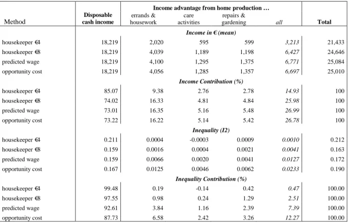
Income Advantages from Home Production
Even though almost everyone enjoys income from some sort of home production, it may not all be similar in value. Thus, in Table 6 we report income shares for each quintile in the base-line model (column A) as well as after adding fictitious income from home production using the various approaches in columns B1, B2, etc. The lowest income quintile benefits consid-erably from home production in relative terms, with its income share rising from 8% in the baseline model to about 10% after including a value for home production. The second and third quintiles also expand their respective share of overall income, whereas the income share of the higher income quintiles is reduced accordingly by several percentage points.
When comparing the distributional impact of home production as based on the two different housekeeper wage approaches, we find a very pronounced equalizing effect when applying a wage rate of €8, and the least equalizing effect for the wage rate of €4 per hour.
4 Empirical Results: the Impact of Home Production on Income Inequality
The predicted wage and the opportunity cost approach range in between, with the opportunity cost approach yielding results similar to the €4 housekeeper wage. These results reflect that individuals with a high baseline income also tend to exhibit characteristics that are linked to a higher predicted wage. The ranking of the approaches according to the strength of the inequal-ity-reducing effect is also mirrored in the fact that the correlation between disposable baseline income and the fictitious income derived from home production is highest (0.22) for the op-portunity cost approach, modest (0.09) for the predicted wage approach, and even slightly negative (-0.03) for the housekeeper wage approach.
Columns C1, C2, etc. give the average percentage increase in disposable income when adding the value of home production according to the various approaches. For the €4 house-keeper wage approach, the cash value of total home production is about 17.5% of the baseline income for the entire population, and about twice as strong in the €8 housekeeper wage as well as in the predicted wage and the opportunity cost approach. As expected, the effect of home production is much greater among the lowest incomes: in fact, in the poorest quintile, home production “adds” 40% of baseline income (and 70-80% in the two other approaches) whereas the top quintile enjoys “only” an increase of 9-23%, respectively.
More interestingly, columns D1, D2, etc. give the average value of equivalent income bound in home production for the different measurement methods. While for the housekeeper wage approaches the added value from home production is hump-shaped across the income distribution, we find a consistently increasing average amount for the predicted wage and the opportunity cost approach. This pattern is influenced by two effects: on the one hand, the number of hours spent on home production is highest in the middle income quintiles (see also column G in Table 5). On the other hand, (current and predicted) wages among high-income households are higher than among less well-off households, reflecting that individuals in rich
4 Empirical Results: the Impact of Home Production on Income Inequality
19
households tend to have characteristics yielding higher earning potentials. In the predicted wage and opportunity cost approach, this latter effect overrides the slightly hump-shaped distribution of the amount of time spent for home production.
4.3
Impact on Income Distribution and Poverty
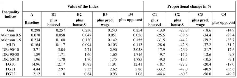
Column A in Table 7 provides a comprehensive picture of inequality and relative poverty using the baseline income measure. We compare these results to those obtained from the amplified income. In general, adding the fictitious value for home production yields the ex-pected and consistent pattern of reduced inequality and poverty, irrespective of the approach chosen.
Again, comparing the various approaches yields a robust ordering, with the strongest inequality reducing effect for the €8 housekeeper wage, and a subsequently declining strength of this leveling effect when applying the predicted wage, the opportunity cost and, lastly, the €4 housekeeper wage approach. For example, the Gini coefficient is cut down by 14% (€4 wage rate), 15% (opportunity cost), 19% (predicted wage) and 23% (€8 wage rate), respec-tively. The results for the decile ratios indicate that this effect is driven similarly by changes in the upper as well as in the lower half of the distribution. The results for relative poverty as measured by the FGT index (see Foster, Greer and Thorbecke 1984)—based on a dynamically adjusted poverty threshold—show the same pattern. The head count poverty ratio (FGT0) is reduced from 15% (baseline income) to less than 11% after adding fictitious income from home production based on the €8 housekeeper wage approach. For all other approaches, the reduction effect is smaller, and smallest for the opportunity cost approach. However, the pov-erty reduction effect is monotonically increasing in the povpov-erty aversion parameter alpha.
4 Empirical Results: the Impact of Home Production on Income Inequality
An alternative presentation of these findings is given in Figure 1, where the Lorenz curve for the baseline income distribution at all points is clearly to the right of the correspond-ing graphs uscorrespond-ing the three alternatively enriched income measures. At the same time the Lo-renz curve for the predicted wage approach always lies in between the two “housekeeper wage” curves, i.e., there are no intersections of these graphs.
4.4
Decomposition of Inequality and Poverty by Socio-Economic Structure
Finally, Tables 8 and 9 provide some insight as to which societal subgroups might actually profit most from home production.12 So far, the sensitivity and robustness analyses showed a
consistent ordering of the various approaches. In order to reduce the complexity of the follow-ing tables, we refrain from presentfollow-ing the results for the housekeeper wage approach based on €8 per hour and the opportunity cost approach in Table 8.
Looking at decomposition by household type, the figures on income levels and ine-quality given in Table 8 show family households with dependent children, in particular mo-noparental households, as well as elderly people (singles and couples) to profit most from the additional consideration of income from home production. In the former case, this is obvi-ously driven by accounting for childcare as one form of home production. With respect to the socio-economic status of the household head, it is the unemployed and pensioners who im-prove their relative income position, while white-collar workers and the self-employed lose in relative terms. To complete the picture, highly educated households lose and the least-educated households gain in relative terms. All this yields the conclusion that households with lower cash incomes profit (also due to the low base effect when calculating relative changes) while households highly engaged in the labor market gain less because they invest less time in
12 All statistical analysis have been conducted using Stata version 9.2, and the decomposition add-ons INEQFAC, IN-EQDECO, and POVDECO, all written by Stephen Jenkins.
4 Empirical Results: the Impact of Home Production on Income Inequality
21
home production due to the higher opportunity costs. Obviously, this cumulates in an overall reduction of income inequality as shown above.
Decomposing inequality (measured by the MLD) in between-groups and within-group inequality generally shows that the former is reduced even more than the latter. However, the exception here is inequality across educational levels of the household head, which shows that adding home production clearly increases the relative contribution of the between-group ine-quality across educational levels when using the predicted wage approach, whereas there is no change when applying the housekeeper wage rate of €4 per hour. For all other grouping vari-ables, the relative contribution of the between-groups inequality remains basically unchanged or, if anything, slightly declines.
Results on the impact of home production on relative poverty (see Table 9) are by and large consistent with the findings on inequality. However, there are some group-specific de-viations. Whereas overall poverty is significantly reduced when including fictitious income from home production, this does not hold for all social groups. In particular, white-collar households exhibit no changes in poverty when applying the first three approaches, and there is even an increase in the poverty head-count ratio from the rather low baseline level of 4.9% to 5.6% based on the opportunity cost approach. For the elderly, there appears to be a reduc-tion in poverty only based on the housekeeper wage approach, but not so for the opportunity cost and predicted wage approach. This is linked to the diminishing effect of higher age in the wage prediction. Looking at differences across the educational levels of household heads, more highly educated households again exhibit an exceptional pattern of stronger reductions in poverty for the predicted wage approach than for the opportunity cost approach.
Decomposing total inequality by income component (factor decomposition – see Table 10) shows that the overall contribution of the added value for home production to total
ine-5 Conclusion
quality of the extended income measure is close to zero. This is particularly the case for the €4 housekeeper wage approach, with almost 99.5% of total inequality being attributable to the money measure of disposable income. Although the share of the fictitious income from home production amounts to one-quarter of the extended income measure for the three other ap-proaches, the contribution to inequality is still below 10% for the €8 housekeeper wage and predicted wage approach, and reaches a maximum of 12% for the opportunity cost approach.
In any case, the contribution of each of the home production activities is of positive value or (almost) zero otherwise. This suggests that individual welfare provided by home production activities is also unevenly distributed, at least to some extent. This is particularly the case within the framework of the opportunity cost approach, and for errands and house-work. Care activities, although unevenly distributed among the population, do not contribute to total inequality in significant terms.
5
Conclusion
This paper supports claims of cash income being a less than perfect measure of individual well-being, and clearly underscores the need to consider non-cash income advantages arising from various home production activities. Our empirical analyses for Germany reveal that basically the entire population profits from at least one household member doing unpaid work at home. Nevertheless, there is quite some variation across socio-economic and demographic characteristics. In line with the international literature, as well as with national findings about the distributional impact of other non-cash components13, we find inequality and poverty in an
extended welfare measure to be by and large lower than in a purely cash-based approach (see
13 See Frick et al. (2006) for non-cash income bound in public educational transfers, Frick et al. (2007a, 2007b) for imputed rent and Frick et al. (2008) for public health transfers, respectively. All these analyses refer to the same population used in the paper at hand, which allows for a comprehensive analysis of the impact of non-cash incomes from four different sources on the income distribution in Germany in 2002 (see Frick et al. 2009).
5 Conclusion
23
also Gottschalk and Smeeding 1997). Sensitivity analyses and robustness checks comparing results obtained from different approaches to measure home production do provide indica-tions of methodological effects arising from the choice of the method. Although the substan-tive notion of reduced inequality in well-being is quite stable, the degree of variation in our findings confirms the need for a harmonized approach in cross-nationally comparative re-search.
This paper proposes a new specification for measuring the monetary value of home production that comprises two distinct features: First, we adjust the numbers of hours spent on home production to reduce bias arising from multi-tasking and, more important, to incorpo-rate diminishing marginal productivity. Second, the proposed predicted wage approach ap-proximates the hourly wage rate for home production by means of the predicted wages of all individuals, rather then using “true” market wages from paid employment. The predicted wage approach thus accounts for rather general, predicted differences in individual productiv-ity and earnings capacproductiv-ity. This is grounded in the consideration that people engaging in home production activities typically act as “amateurs,” lacking professional skills in the things they do at home—whatever professional skills they may otherwise possess. By means of these two features—adjusting the underlying time measure and predicting individual productivity and opportunity—the proposed predicted wage approach yields a more robust measure of the economic utility derived from home production, in terms of the underlying assumption as well as the estimation results.
6 References
6
References
Anger, Silke (2006): Zur Vergütung von Überstunden in Deutschland: Unbezahlte Mehrarbeit auf dem Vormarsch. Wochenbericht des DIW Berlin 15/16: 189-196.
Aslaksen, Iulie, and Charlotte Koren (1996): Unpaid household work and the distribution of extended income: The Norwegian experience. Feminist Economics 2(3): 65-80.
Beblo, Miriam (1999): Bargaining over Time Allocation. Economic Modeling and Econometric Inves-tigation of Time Use within Families, Heidelberg, New York.
Blundell, R., Preston, I. and Walker, I. (eds.) (1994): The Measurement of Household Welfare, Cam-bridge University Press, CamCam-bridge.
Bonke, Jens (1992): Distribution of economic resources: Implications of including household produc-tion. Review of Income and Wealth 38(3): 281–293.
Burda, M. C., and D. S. Hamermesh (2009): Unemployment, Market Work and Household Produc-tion. IZA Discussion Paper No. 3955, Institute for the Study of Labor, Bonn, January 2009 Bryant, W. Keith, and Cathleen D. Zick (1985): Income distribution implications of rural household
production. American Journal of Agricultural Economics 65: 1100–1104.
Bryant, W. Keith, Hyojin Kang, Cathleen D. Zick and Anna Y. Chan (2004): Measuring Housework in Time Use Surveys. Review of Economics of the Household 2(1): 23-47.
Bundesministerium für Familie, Senioren, Frauen und Jugend (BMFSFJ), Statistisches Bundesamt (StaBua) (Hg) (2003): Wo bleibt die Zeit? Die Zeitverwendung der Bevölkerung in Deutsch-land 2001/02, Wiesbaden.
Canberra Group (2001) Expert Group on Household Income Statistics: Final Report and Recommen-dations, Ottawa.
Chadeau, Ann (1992): What is households’ non-market production worth? OECD Economic Studies 136: 29-55.
Fazis, Harley, and Jay Steward (2006): How Does Household Production Affect Earnings Inequality? Evidence from the American Time Use Survey. BLS Working Paper 393
Foster, J., Greer, J. and Thorbecke, E. (1984): A Class of Decomposable Poverty Measures.
Econo-metrica 52(3): 761-766.
Frick, J. R., Grabka, M.M. and Groh-Samberg, O. (2006): Estimates of Public Educational Transfers and Analysis of their Distributional Impact in Germany. (National Report. Research project “Accurate Income Measurement for the Assessment of Public Policies” (AIM-AP), DIW Ber-lin: Berlin.
Frick, J. R., Goebel, J., and Grabka, M. M. (2007a): Assessing the Distributional Impact of "Imputed Rent" and "Non-Cash Employee Income" in Microdata: Case Studies Based on EU-SILC (2004) and SOEP (2002). In: Eurostat (eds): Comparative EU statistics on Income and Living Conditions: Issues and Challenges. Proceedings of the EU-SILC Conference, Helsinki, 6-8 November 2006, European Communities: Luxembourg, 117-142.
Frick, J. R., Grabka, M.M. and Groh-Samberg, O. (2007b): Estimates of Imputed Rent and Analysis of their Distributional Impact in Germany. (National Report. Research project “Accurate Income Measurement for the Assessment of Public Policies” (AIM-AP) , DIW Berlin: Berlin.
Frick, J. R., Grabka, M.M. and Groh-Samberg, O. (2008): Estimates of Health Related Transfers and Analysis of their Distributional Impact in Germany. (National Report. Research project “Ac-curate Income Measurement for the Assessment of Public Policies” (AIM-AP), DIW Berlin: Berlin.
Frick, J. R., Grabka, M.M. and Groh-Samberg, O. (2009): Aggregate Estimates of Non-Cash Income Components and Analysis of their Distributional Impact in Germany (National Report.
Re-6 References
25
search project “Accurate Income Measurement for the Assessment of Public Policies” (AIM-AP), DIW Berlin: Berlin.
Gørtz, Mette (2007): Household Production in the Family – Work or Pleasure?, Paper presented at Seminar at Schumpeter Institute, Humboldt University, December 2007, Berlin
Gottschalk, P. and Smeeding, T. M. (1997): Cross-National Comparisons of Earnings and Income Inequality. Journal of Economic Literature, XXXV, 633-687.
Gottschalk, Peter, and Susan E. Mayer (2002): Changes in home production and trends in economic inequality. In: Daniel Cohen, Thomas Piketty, and Gilles Saint-Paul (Eds.): The new econom-ics of rising inequality, Oxford: Oxford University Press, 265-284.
Gronau, R. (1980): Home Production – A Forgotten Industry. The Review of Economics and Statistics 62(3): 408-416.
Ironmonger, Duncan (1996): Counting outputs, capital inputs and caring labor: Estimating gross household product. Feminist Economics 2(3): 37-64.
Jenkins, S. P and O'Leary, N. C (1996): Household Income Plus Household Production: The Distribu-tion of Extended Income in the U.K. Review of Income and Wealth 42(4): 401-419.
Kooreman, P. and Wunderink, S. (1997): The Economics of Household Behaviour, Macmillan Press Ltd, London.
Koutsambelas, Christos, and Panos Tsakloglou (2008): Distributional effects of consumption of own production and fringe benefits: Greece 2004. (National Report. Research project “Accurate In-come Measurement for the Assessment of Public Policies”.
Lewis, J., Campbell, M. and Huerta, C. (2008): Patterns of paid and unpaid work in Western Europe: gender, commodification, preferences and the implications for policy, Journal of European
Social Policy 18(1): 21–37.
OECD (1995): Household production in OECD countries - Data sources and measurement methods. By France Caillavet, Ann Chadeau, and F. Coré.
OECD (2006): Understanding National Accounts. By François Lequiller Derek Blades. Pierce, B. (2001): Compensation Inequality. Quarterly Journal of Economics, p. 1493-1525. Reid, Margaret G. (1934): Economics of Household Production. New York: John Wiley.
Saunders, Peter et al. (1992) Non-cash Income, Living Standards, Inequality and Poverty: Evidence from the Luxembourg Income Study, Discussion Papers No. 35, Social Policy Research Cen-tre (SPRC), The University of New South Wales, Australia.
Schaffer, A. und Stahmer, C. (2006): Extended Gender-GDP – A Gender-Specific Analysis of Tradi-tional GDP and Household Production in Germany, Jahrbücher für NaTradi-tionalökonomie und
Statistik, 226/3: 308-328.
Smeeding, T. M. and D. H. Weinberg (2001): Toward a Uniform Definition of Household Income.
The Review of Income and Wealth 47(1): 1-24.
Swiebel, Joke (1999): Unpaid Work and Policy-Making. Towards a Broader Perspective of Work and Employment. DESA Discussion Paper No. 4, United Nations, Department of Economic and Social Affairs
Wagner, G..G., Frick, J.R., and Schupp, J. (2007): The German Socio-Economic Panel Study (SOEP) - Evolution, Scope and Enhancements. Schmoller’s Jahrbuch - Journal of Applied Social
Sci-ence Studies 127 (1): 139-169.
Wrohlich, K. (2007): Evaluating Family Policy Reforms Using Behavioral Microsimulation. The Example of Childcare and Income Tax Reforms in Germany. Doctoral Thesis, Free University Berlin, 2007. Published on-line: http://www.diss.fu-berlin.de/2007/531.
Zick, Cathleen D., and W. Keith Bryant (1990): Shadow Wage Assessments of the Value of Home Production: Patterns from the 1970's. Lifestyles: Family and Economic Issues 11(2): 143-160. Zick, Cathleen D., W. Keith Bryant, and Sivithee Srisukhumbowornchai (2008): Does housework
matter anymore? The shifting impact of housework on economic inequality. Review of the
7 Tables
7
Tables
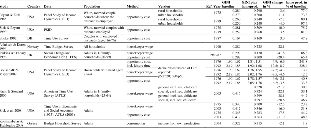
Table 1: Previous Studies on the Distributional Effect of Home Production
Study Country Data Population Method Version Ref. Year
GINI baseline GINI plus homeprod. GINI change in %
home prod. in % of baseline
rural households 0.280 0.290 3.6 77.0
urban households 1975 0.270 0.300 11.1 73.3
rural households 0.260 0.240 -7.7 80.1
Bryant & Zick
1985 USA
Panel Study of Income Dynamics (PSID)
White, married-couple households where the husband is employed
opportunity cost
urban households 1979 0.250 0.240 -4.0 97.4
1975 0.281 0.309 10.0 75.7
Zick & Bryant
1990 USA PSID
White, married couples with
husband employed opportunity cost 1979 0.259 0.268 3.5 81.0
Bonke 1992 DK Time Use Survey Couples with employed
husbands (aged 16-76) opportunity cost 1987 0.164 0.169 3.0 47.8
Aslaksen & Koren
1996 Norway Time Budget Survey All households housekeeper wage 1990 0.289 0.225 -22.1 --
housekeeper wage 0.292 0.170 -41.8 86.3
Jenkins & O'Leary
1996 UK
Social Change and Economic Life (+ FES)
Adults in
1-family-households (20-59) opportunity cost 1986/87 0.292 0.209 -28.4 65.4
1976 1.90; 1.62 1.81; 1.51 -4.9; -6.6 241.8 opportunity cost,
incl. leisure time 1992 2.19; 1.85 1.92; 1.68 -12.5; -8.7 228.4
1976 1.90; 1.62 1.76; 1.55 -7.2; -4.3 13.9 housekeeper wage
1992 2.19; 1.85 2.02; 1.76 -7.5; -4.6 12.5 1976 1.90; 1.62 1.78; 1.57 -6.6; -3.1 40.8 Gottschalk &
Mayer 2002 USA
Panel Study of Income Dynamics (PSID)
Households with head aged 25-64
opportunity cost
decile ratios instead of Gini reported:
p50/p20; p80/p50
1992 2.19; 1.85 2.05; 1.78 -6.2; -3.5 33.3
general, excl. sec. childcare 0.328 -21.2 30.5
special, excl. sec. childcare 0.324 -22.1 33.1
general, incl. sec. childcare 0.299 -28.1 44.7
Fazis & Steward
2006 USA
American Time Use Survey (ATUS)
Adults in
1-family-households (25-64) housekeeper wage
special, incl. sec. childcare
2003 0.416
0.297 -28.6 46.7
1975 0.343 0.300 -12.5 23.2
housekeeper wage
2003 0.412 0.346 -16.0 31.8
1975 0.343 0.283 -17.5 44.9
Zick et al. 2008 USA
Time Use in Economic and Social Accounts (1975), ATUS (2003)
Adults
opportunity cost
2003 0.412 0.363 -11.9 48.5
Koutsambelas &
7 Tables
27
Table 2: Home Production Activities by Selected Household Characteristics in Germany, 2002
Average number of hours per normal week day spent in …
Household characteristics
Total Home
Production Errands Housework Childcare Elderly care
Repairs & Gardening yes 6.1 [9.5] 1.6 [1.9] 2.1 [3.4] 0.9 [2.0] 0.2 [0.3] 1.4 [1.9] Garden
no 4.3 [6.4] 1.4 [1.7] 1.7 [2.6] 0.5 [1.2] 0.1 [0.2] 0.5 [0.7] yes 6.4 [9.7] 1.7 [2.0] 2.1 [3.5] 0.8 [1.9] 0.2 [0.3] 1.5 [2.1] Home
owner no 4.5 [6.9] 1.4 [1.7] 1.7 [2.7] 0.6 [1.5] 0.1 [0.2] 0.6 [0.8] < 2.000 6.3 [9.9] 1.7 [2.0] 2.1 [3.5] 0.8 [2.0] 0.1 [0.3] 1.5 [2.1] 2.000 - 500.000 5.4 [8.3] 1.5 [1.8] 1.9 [3.1] 0.7 [1.8] 0.1 [0.2] 1.0 [1.4] Community
size
> 500.000 4.3 [6.3] 1.4 [1.7] 1.7 [2.5] 0.5 [1.2] 0.1 [0.2] 0.6 [0.7] West 5.2 [8.0] 1.5 [1.8] 1.9 [3.0] 0.7 [1.8] 0.1 [0.2] 1.0 [1.2] Region
East 5.6 [8.3] 1.7 [2.1] 2.0 [3.0] 0.6 [1.2] 0.1 [0.3] 1.2 [1.7] no 4.6 [6.3] 1.5 [1.8] 1.8 [2.9] 0.1 [0.2] 0.1 [0.2] 1.0 [1.3] Children in
hh yes 8.1 [14.9] 1.7 [2.0] 2.2 [3.7] 3.0 [7.6] 0.1 [0.2] 1.1 [1.3]
Total 5.3 [8.1] 1.5 [1.8] 1.9 [3.0] 0.7 [1.7] 0.1 [0.2] 1.0 [1.3]
[x.x] values in brackets give the respective number of hours before correction. Corrections include imputation for missing values in cases of item non-response, top-coding at 16 hours a day for each activity and accounting for multiple activities by taking the square root of hours spent in each activity.
Population: Private households.
7 Tables
Table 3: Home Production by Selected Individual Characteristics in Germany, 2002
Personal
characteristics
individually engaged in home production %
hours spent in home production “before correction”
“corrected” hours spent in home production
Sex male 91.3 3.3 2.6
female 97.0 6.2 3.7
Age group 17-24 82.2 2.5 1.9
25-40 95.5 6.0 3.5
41-55 96.0 4.6 3.2
56-65 96.0 4.7 3.2
> 66 95.7 4.9 3.2
Marital status married 96.0 5.7 3.5
single 89.1 3.0 2.3
divorced 96.9 4.8 3.2
widowed 95.8 4.7 3.2
Migration background no 94.5 4.8 3.2
yes 92.9 5.3 3.2
Health status very good 90.1 3.8 2.7
good 94.5 4.7 3.1
satisfying 96.4 5.2 3.4
not so good 94.7 5.2 3.3
bad 83.2 4.1 2.6
General schooling lower secondary 94.1 5.0 3.2
intermediate 95.1 5.0 3.3
college 93.9 4.1 2.9
Vocational education none 90.7 4.5 2.9
basic vocational 96.1 5.3 3.4
higher vocational 95.2 4.4 3.1
tertiary 94.3 4.0 2.9
Unemployed no 94.0 4.7 3.1
yes 98.6 6.4 3.9
Employment status fulltime 93.5 3.1 2.5
part time 99.1 6.5 4.0
training 80.2 2.1 1.8
irregular 94.3 6.4 3.7
not working 94.9 6.0 3.6
Total Population 94.3 4.8 3.2
Population: Persons aged 17 and over in private households.