Object Search and Localization
for an Indoor Mobile Robot
Kristoffer Sj¨o, Dorian G´alvez L´opez, Chandana Paul,
Patric Jensfelt and Danica Kragic
Centre for Autonomous Systems, Royal Institute of Technology, Stockholm, Sweden
In this paper we present a method for search and localization of objects with a mobile robot using a monocular camera with zoom capabilities. We show how to overcome the limitations of low resolution images in object recognition by utilizing a combination of an attention mechanism and zooming as the first steps in the recognition process. The attention mechanism is based on receptive field cooccurrence histograms and the object recognition on SIFT feature matching. We present two methods for estimating the distance to the objects which serve both as the input to the control of the zoom and the final object localization. Through extensive experiments in a realistic environment, we highlight the strengths and weaknesses of both methods. To evaluate the usefulness of the method we also present results from experiments with an integrated system where a global sensing plan is generated based on view planning to let the camera cover the space on a per room basis.
Keywords: spatial mapping, object search, visual search, view planning
1. Introduction
The field of mobile robotics is continuously ex-panding. The question is no longer if robots will take the leap out of the factories and into our homes, but when. The future applications of autonomous agents require not only the abil-ity to move about in the environment and avoid obstacles, but also the ability to detect and rec-ognize objects and interact with them. Yet most robotic applications tend to be one of the two: Either entirely blind to everything in their sur-roundings except what is required merely for navigating through the environment, or else de-signed to function in a fixed setting, where they have a well-known and unchanging frame of reference that they can relate objects to. Never-theless, there are some recent attempts to
over-come these limitations. For example, the robot league of the Semantic Robot Vision Challenge
(SRVC) [12]is a promising attempt to advance understanding and development in this area. The topic in this paper contributes to the field in that it deals with object search and detection in realistic indoor environments and thus aims at reducing the aforementioned limitations.
is described. It utilizes receptive field cooccur-rence histograms (RFCH), which provide dif-ferent hypotheses for any occurrence of each object in the image. Zooming in combination with controlling the pan/tilt-angles is used to provide a closer view of the objects for the later recognition step which is performed using SIFT feature matching.
To perform an efficient object search and de-tection in a realistically-sized environment, the robot needs the ability to plan when and from where to acquire images of the environment, as exhaustive search is unfeasible. View planning is a comparatively old, but still thriving research area. Early work on view planning was of a mostly theoretical nature, but as the field has matured more implementation-oriented results are emerging. [15] examines the problem of optimally covering the “view sphere”, i.e. all angles that can be seen from a fixed point in space, given a probability distribution for the presence of the object. In[16], the approach is augmented with multiple viewpoints, each next point selected by a greedy policy. The gen-eral problem of finding a minimal set of view-points from which to observe all parts of the environment is called theart gallery problem.
[8] proves that this problem is NP-hard, and thus approximate solutions are required. Us-ing a polygonal map of the robot’s surroundUs-ing,
[5]uses a sampling scheme to find an approx-imate solution to the art gallery problem while additionally taking into account the practical limitations of sensors by postulating maximum and minimum distance and maximum viewing angle. However, parameters for only a single object are considered.
Another related view planning problem is the watchman problem, which entails computing a minimal continuous path through space from which all of the environment can be seen; here, the length of the path is what is crucial - in con-trast to the art gallery problem, where the dis-tance between viewpoints is immaterial. The watchman problem, too, is NP-hard when there are “holes” in the free space(as shown in[1]). Many different approaches exist to solving both the art gallery and watchman problems; [11]
provides an extensive survey. In [13], the cost of moving and processing views is combined in a single planning task, approximated as an in-teger linear problem(ILP). A set of candidate view points is assumed to be provided.
1.1. Contributions
Using a combination of view planning and vi-sual search, we show how existing computer vision methods can be used on a mobile robot platform to produce an autonomous system that is able to efficiently detect and localize differ-ent objects in a realistic indoor setting. The proposed system is implemented on a mobile robot and its practicability is demonstrated in experiments.
We build further on the ideas presented in [2]. For the local visual search we add a vision-based object distance estimate that facilitates better zooming capabilities. In [2] distances to objects were estimated using a laser scan-ner. We also improve the way multiple objects can be searched for at the same time through better utilization of shared zooming. We also add a more efficient view planning strategy that takes into account the layout of the environment and the specific constraint of the individual ob-jects. Finally, we present results from an exten-sive experimental evaluation of the vision based distance estimation and show examples of runs with the entire integrated system.
1.2. Hardware
The robotic platform used is a Performance PeopleBot. It is equipped with a SICK laser rangefinder with a 180 degree field, positioned near the floor (at about 30 cm), and with a Canon VC-C4R video camera, able to acquire low resolution images(320×240 pixels)with pan/tilt functionality and up to 13× magnifica-tion. The camera is mounted about 1m above the floor. The robot has a differential drive and a wireless LAN connection.
2. Navigation
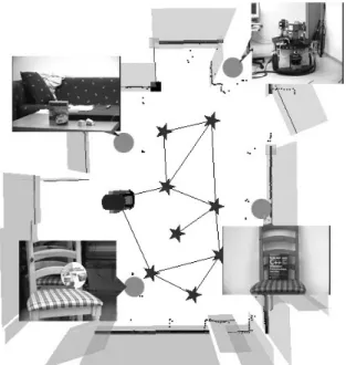
them, constituting a navigation graph which represents known robot-navigable space. Sim-ilar ideas have been presented in [7]. This is performed in the mapping step; as the robot moves into unexplored areas, it drops nodes at regular intervals, and when it moves between existing nodes it connects them in the map. For example, consider the situation in Figure 1. It represents the map of a room built by means of laser data, where stars and lines represent the navigation graph created during exploration. The figure also shows some objects placed at different positions in the room. The objective of the object search algorithm presented further on in the paper is to detect all the objects, with-out prior information abwith-out their location, while keeping the trajectory traveled during the search short.
Figure 1. Example of distribution of objects in a room. Stars represent nodes, and circles, the actual positions of
objects.
The object search begins with a planning step used to determine an efficient movement policy for exploring the map. In the current system, only the navigation nodes are considered dur-ing planndur-ing, as they are the only parts of the map guaranteed to be reachable. This way, the process is also computationally cheaper. The map used in the search procedure repre-sents a room, i.e. a more or less convex space, that consists of different types of geometrical structures such as walls, furniture, etc. Starting
originally with a more complex map of the envi-ronment, the maps of single rooms are obtained by dividing the navigation graph into subgraphs by cutting out all the door nodes[7]. All fea-tures of the map are assigned to the room which has the nearest navigation node. Planning ef-ficient movement between rooms is currently performed using a next-closest-room-first strat-egy.
The resulting navigation plan provides the robot with a list of nodes it needs to visit. For each node, there is also a list of viewing directions or views that it needs to process as well as the list of objects it has to look for in each view. The navigation plan is defined so that all parts of the room are searched for all the objects, while keeping the number of visited nodes and visual searches as low as possible. Additional object constraints must also be ful-filled as, for example, a small object can only be detected/recognized from a short distance. Finally, uniqueness must be taken into account: objects should be discarded once they are found, which means the exploration plan will need to be updated.
2.1. Grid-based View Planning
2.1.1. Occupancy Grid
The metric map built using SLAM is not ge-ometrically perfect. Features extracted from laser data do not form a clean, continuous out-line. Typically, different and commonly over-lapping line features explain the same sensor data thus making the resulting clutter to increase planning complexity. For this reason, a simpler occupancy grid-based representation is used as the base for the view planning. The occupancy grid can be acquired either directly from laser data or by rasterizing an existing feature map by simply marking a cell as occupied if it contains a feature.
computational cost. Small cells will be very closely packed and thus grouped into the same viewing directions for the robot to process. On the other hand, a too-large cell size will lead to insufficient detail in the plan and the robot may miss parts of the map to explore. In the current system, a fixed cell size of 0.5m is used.
2.1.2. Views
Using the grid,viewscan be calculated. A view is a triplet consisting of the map node to which the robot has to travel, the direction it should point its camera to and the list of objects to be searched for in the resulting image. In order to simplify the calculations, grid cells are con-sidered visible in a view if their center point is inside the field of view of the robot.
2.1.3. Object Constraints
There are various objects the robot has to look for and their attributes must be taken into ac-count; specifically, their size, since it affects the distance from which an object can be de-tected/recognized. Hence, for each object a minimum and a maximum distance value is de-fined; the robot should attempt to find it only at distances in this interval.
There are separate distance constraints for ob-ject recognition and obob-ject detection. For recog-nition, the minimum distance is simply defined as the range at which the object would fill an entire image with a default zoom. The maxi-mum distance is defined as the range at which the object would occupy an entire image if max-imum zoom was used. The minmax-imum distance for purposes of detection is given by the param-eters of the detection algorithm, explained in more detail in Section 3.2.
Figure 2 shows an example of two potential views of a set of cells that, in this case, originate from a wall. Large circles represent nodes; dots, grid cell centers; the numbers close to them, the nodes they are associated with; and the shaded area, the views(along with objects planned for in each view). Note how views from both the nodes 15 and 18 are needed in order to cover the right-hand wall due to the different sizes of the objects. Other parts of the map are covered by different sets of nodes.
Figure 2.Example of the effect of distance constraints on view planning.
2.1.4. Planning Strategy
The objective of the algorithm is to ensure that any of the sought objects would be seen in at least one of the planned views regardless of which cell it was in – in other words, each pos-sible object-cell combination must be covered by some view.
After generating the grid, the view covering the most object-cell pairs is chosen iteratively until no pair remains that is not covered by any view, or no view remains that covers further pairs. In the latter case, the pairs are impossible to cover given the provided set of nodes. The object-cell pairs covered by each view chosen are removed from subsequent iterations when they are cov-ered by the desired number of views, which is 1 in the simplest case.
2.1.5. Tilt Angle Selection
Since a 2D map of the environment is used, there is no direct information that could help in deciding how to use the tilt angle of the camera. Yet, the objects being sought for might be at any height, and thus some thought must be given to covering the vertical dimension as well as the horizontal ones.
Those grid cells which are closer to a given view’s associated node than a set threshold(here set to 2 meters) generate new views that cover the vertical extent of the objects’ possible lo-cations. Using the average distance for those grid cells, together with an upper and a lower boundary for objects’ positions, one or more tilt angles are selected(with as little overlap as pos-sible)and the resulting views are added to the plan.
3. Vision
To detect objects, the system uses receptive field cooccurrence histograms(RFCH)as described in[2]. As potential objects are detected, the sys-tem calculates suitable interest regions for the camera to zoom on. Here, the system needs an estimate of the distance to the object in order to decide whether to proceed with recognition given the current camera parameters or if zoom-ing is needed. In [2] this estimate was taken from the laser scanner; we, instead, obtain an estimate through the RFCH procedure itself. If the distance allows for reliable recognition immediately, the system uses SIFT feature ma-tching in order to recognize the object[9]. Oth-erwise, the interest regions for the different ob-jects are merged as far as possible and the cam-era zooms in on each region in turn, repeating the procedure until all objects have either been found or eliminated. A detailed description of the above procedure is presented in the follow-ing sections.
3.1. Object Search Algorithm
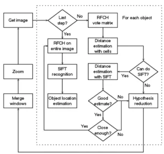
Figure 3 presents the object search procedure as a whole. Starting with an image at 1× magnification, each object is processed inde-pendently, whereupon the resulting zoom win-dows are merged and each gives rise to a new,
Figure 3.Object search algorithm.
zoomed image and the procedure repeats for each of them.
The algorithm has three steps: initial, middle and final. It progresses through them according to the following:
• Initial: No magnification used. After dis-tance estimation and zooming, it proceeds to the middle step.
• Middle: Magnification given by output from zoom window sharing(Subsection 3.4.2). If new distance estimate indicates current mag-nification is too small (not within 1.8× of new desired middle magnification), this step is repeated. If, on the other hand, it is within 1.2× of the desired final magnification, it skips straight to recognition. Otherwise, it moves to final step without further zooming.
• Final: Magnification in accordance with Eq. 1. Recognition performed.
Typically, each step will run once only.
reduction (Subsection 3.4.1) prunes the result for each object; then, hypothesis sets for the different objects are merged.
The magnification required for the algorithm to jump to the recognition stage is a tuning param-eter; in the current system, it is set to 1.2× of the final. There is also a “short-cut” that lets the object go straight from step 1 to step 3 if the current magnification is found to be essen-tially equal to the middle magnification(within 1.8×).
The last step in the object search consists sim-ply of recognition, wherein SIFT matching is preceded by a “sanity check” RFCH match on the entire image(see Subsection 3.5). If the ob-ject is found, its location in space is computed from its position in the image and the distance estimate. The output of the algorithm is a list of objects that were found in the current view and their calculated locations and distances.
3.2. Object Detection
The detection process works on a per-object ba-sis and conba-sists of several steps: an image is first taken by the camera and divided into cells. For each cell, RFCHs are computed using clusters learned from each respective object in a train-ing phase. These are then matched against the training images’ histograms, resulting in a sim-ilarity value for each cell and object. This set of cell values is called the object’svote matrix. An example is shown in Figure 4. Higher value of cells(represented by a lighter shade in the im-age)denotes a greater degree of correspondence between test image and training image.
Next, object hypotheses are generated. A cell is a hypothesis if its value is higher than those of its 8-connected neighbors, as well as higher than an object-dependent threshold. The size of the vote cells in the above algorithm is a tuning parameter. Large cells mean faster histogram matching; however, they decrease the detection rate when they are larger than the objects in the initial image. Also, maximum distance allowed for object detection during the planning step is set to the distance at which an object would oc-cupy a single cell at no zoom, which decreases as cell size grows. The value used in our work, 15×15 pixels, is a compromise between these considerations.
a)The book is the object the robot searches for.
b)The vote matrix for the book in the above image.
Figure 4.Vote matrix(b)generated from image(a)
where the object occupies large portion of the image. The lighter a cell, the higher probability of the object.
3.3. Distance Estimation
might be inaccurate. To address these issues, in this work we use two alternative ways for dis-tance estimation.
Figure 5.Distance estimation provided by the laser may not be reliable: instead of the distance to the object on
the table, the distance to the shelf is measured.
3.3.1. Using the Vote Matrix
Using the RFCH vote matrix for distance esti-mation consists of measuring how many cells are part of the object and treating the area they occupy in the image as an approximation of the object’s size. Here, cells are considered to be associated with a hypothesis if their degree of match is above the threshold and if there is an 8-connected path to the hypothesis with cells of monotonically increasing value. Only the strongest hypothesis and its associated 8-connected cells are taken into account, because it is likely to be the most reliable.
Given the object’s actual size stored in the train-ing database, the distance is then computed as:
D=
Wreal2WDim vote
tanα 2
whereDstands for the estimated distance( me-ters); Wreal, for the real width of the object
(meters); Wim, for the width in pixels of the
camera image;Dvote, for the width in pixels of
the bounding box of the cells associated with a hypothesis andα, the horizontal viewing an-gle. This procedure is fast and approximate, but sufficiently accurate to allow the object search algorithm to assign a valid zoom.
3.3.2. Using SIFT
SIFT produces a scale parameter for each key point extracted. For each matched pair of key points in the training and recognition image, the quotient of the keys’ scale parameter gives an estimate of their relative apparent size and hence their distance, according to:
D=
Wreal2WWim tr
Str Sreal
tanα 2
whereStrdenotes the scale of the point extracted
from the training image; Sreal, the scale of the
point extracted from the recognition image, and Wtr, the width of the object in the training image
in pixels.
As mis-matched key point pairs can produce in-correct scale parameters, the final estimate of the object distance is taken as the median of the distance estimates from all matches. Ex-periments indicate that an adequate estimate is obtained given 10 or more SIFT matches. With 4 matches or more, a passable rough estimate is typically obtained(within about 30%). If there are fewer than 4 matches, the result is likely to be very poor(most likely based on some other structure than the object)and is not used.
The drawback of the above method is that ex-tracting SIFT features from an image is compu-tationally expensive, and using it to guide the zoom process may take too long to be feasible. Another problem is the number of SIFT features required to obtain a robust estimation; when the object is small in the image (i.e. resolved by few pixels), it is unlikely that enough matches will be available.
3.4. Calculation of Zoom
angle of view(α), as well as the vertical (β), are calculated as:
α =2 arc tan
Wreal
2D
β =2 arc tan
Hreal
2D
(1)
whereWrealandHrealrepresent the known width
and height of the object.
Since the object will typically not have the same aspect ratio as the image, only one of the angles α and β can be used to select the magnifica-tion parameter. Therefore, of the two levels of magnification suggested by the height and the width respectively, the lower level is selected, as given by the following rule:
If Wim
Wtr <
Him
Htr (Him and Htr being the heights analogous to the widths Wim and Wtr), α is
used; otherwise,β.
3.4.1. Hypothesis Grouping and Reduction
Even with the threshold, there are typically too many hypotheses to evaluate one-by-one. In order to avoid excessive zooming and process-ing, hypotheses are grouped together intozoom windows, which are regions of the image to be magnified and processed. The size of these win-dows is determined by the magnification recom-mended by the distance estimate of the strongest hypothesis. The position of the window is cho-sen to cover the maximum number of hypothe-ses, and this is repeated until all hypotheses are covered.
In cases when the distance parameter is not very accurate, an error propagates into the calcula-tion of the magnificacalcula-tion parameter and into the size of the zoom windows. This may lead to generating more zoom windows than is warranted and, consequently, lengthening the search process. Thus, as a second step it is de-sirable to remove those windows which do not contribute information to the search, as they ei-ther contain too few hypotheses or are located close to “richer” zoom windows. Therefore, zoom windows which overlap more than 20% with another containing at least 3 times its num-ber of hypotheses are removed. These condi-tions are quite conservative in order to ensure that no potentially important zoom windows are removed.
3.4.2. Zoom Window Sharing
When searching for several objects, the set of zoom windows obtained for each object is puted separately. After this is done, the com-bined set of windows needs to be merged to reduce redundant steps. Here, we look for in-stances of a zoom window encompassing that of another object, in which case we can remove the latter.
Not all the zoom windows that overlap can be merged, as straying too far from each object’s target magnification may cause object detec-tion to fail. The object search process has three steps: the first step without zooming, the second step with a middle-level zoom and the third step with large zoom; see Subsection 3.1. It is not as important that the middle-level zoom is exact, since it is only used for hypothesis finding with RFCH. Thus, a maximum and a minimum mag-nification is defined for the middle-level detec-tion step, allowing some flexibility in selecting the windows to be used in this step. It is most important to get the minimum zoom right: the lower it is, the more objects we can look for at one time, but the higher the risk that objects are missed because they appear too small in the image.
The algorithm works as follows: first all zoom windows are shrunk to their minimum size. Then, each zoom window associated with an object A is compared with those of an object B. If the hypotheses contained by one of B’s windows can be made to be contained by one of A’s – expanding the latter if needed, while con-forming its maximum allowed size – then the B window is removed and object B is added to the A window’s list of candidate objects to look for in the next step. This procedure is repeated for each pair of objects. Tests have shown that too flexible a window size tends to be harmful to detection; in this work the maximum middle-level magnification is set to 0.75 of the final zoom level, and the minimum to 0.7 of the final zoom level.
a)An example scene where the rice carton, the book and the mouse pad are searched for.
b)Shared zoom windows.
Figure 6.Shared zoom windows of three objects placed at different distances.
arise from the rice carton; the dark ones, from the book, and the striped ones from the mouse pad. Note that three of the windows contain hypotheses for more than one object.
3.5. Object Recognition
The final object recognition is done once the object occupies either the whole image or a large portion of it. It consists of extracting SIFT features from the current image and matching them with the SIFT features in the training im-age. SIFT features are scale-, position- and rotation invariant up to a certain level, mean-ing that many of the features will match even if the object is seen from a different angle or under different lighting conditions. However, it is
usu-ally the case that the number of SIFT matches during the search is much lower than the num-ber extracted from the training image, due to changes of viewing angle and background. Be-cause of this, we consider an object to have been found if at least a 5% of the SIFT features match. This value has previously been demonstrated to result in few false positives in[2].
Once an object is recognized, its position in the environment is calculated from the pan and tilt angles of the camera, the estimated position of the object inside the image and the distance calculated by the system; see Subsection 3.3. Because of the large variation present in the images, it is very probable that false positives reach the last step of the visual search. In order to reduce the amount of unnecessary extraction of SIFT features, the same RFCH algorithm that is used for detection is used one last time on the fully zoomed image before running the recog-nition algorithm. The SIFT-based recogrecog-nition is performed only if this match is successful.
4. Experimental Evaluation
Several experiments were performed to evalu-ate the proposed algorithms. Test objects used in the experiments are: a book, a rice carton, a printed mouse pad, a printed cup, a box for a trackball, and a large robot. The size of the forward face of the objects varied, from the cup at 14×10 cm to the robot at 63×55 cm. Color and shape were likewise diverse, providing a highly heterogeneous sample.
4.1. Object Detection Using RFCH
The robustness of RFCH object detection was evaluated in the following way:
Five test objects1 (cup, trackball box, rice car-ton, book, mousepad)were placed at eight dif-ferent distances, between 0.5 m and 4 m, from the robot’s camera, using two different back-grounds(a plain white wall and a typical office scene). The robot was excluded in this evalua-tion, as the ranges where it is detected differed too much from the other objects. Five images per position were obtained, introducing some perturbation in the object between each.
1
As described previously, for each image, RFCH was used to calculate the similarity value for each vote cell, and this was thresholded accord-ing to an object dependent threshold. The vote cells whose values were above the threshold were segmented into 8-connected regions and the local maxima of these regions were extracted as hypotheses. The hypotheses were manually labeled as true if they overlapped with a part of the object in the test image, otherwise they were considered false. Figure 7 shows the ratio of false hypotheses generated in the set of test images as a function of distance.
Figure 7.Percentage of false hypotheses generated by the RFCH attention mechanism.
Generally, at larger distances less pixels of the object are visible and it is less distinct from the background. Thus, it can be seen that a larger number of false hypotheses are generated at larger distances. The rate of detection for the objects selected ranges from approximately 65% at close distances, to 35% at longer dis-tances. This sensitivity affects the efficiency of the visual search, as false hypotheses can give rise to unproductive zoom positions, but it also ensures that true hypotheses are very rarely ne-glected.
4.2. Initial Distance Estimation
As mentioned in Subsection 3.3, initially in the visual search an approximate distance estimate is required in order to direct zooming actions and determine when SIFT extraction may be performed. Below are the results highlighting the properties of RFCH and SIFT, respectively, when used for this purpose.
The same set of images was used as in Subsec-tion 4.1, and the distance was computed using both RFCH and SIFT separately for every im-age. The distance estimate from RFCH is based on the strongest hypothesis. The performance of distance estimation is thus affected by how often a correct hypothesis is selected for dis-tance estimation. Figure 8 presents statistics on the likelihood of selecting the correct hy-pothesis for distance estimation as a function of distance.
Figure 8.Percentage of correctly chosen hypotheses for distance estimation.
It is evident that reliability decreases with dis-tance as the signal-to-noise ratio of the image drops. At 2.5 m and above, less than half of the distance estimates are based on the actual object in the image, and performance continues to drop until, at 4 meters, the area used becomes nearly random.
a)RFCH distance estimates.
b)SIFT distance estimates.
Figure 9.Distance estimation results; all objects. Top image RFCH, bottom SIFT. Boxes signify one standard
deviation about the average for each distance; lines signify the most extreme values.
inspecting the average value of the estimates be-yond 2.5 m in Figure 9. b). This is because a certain level of detail is needed to extract SIFT keys. In contrast, RFCH, though most reliable at medium ranges(as demonstrated by the stan-dard deviations in Figure 9. a), retains the ability at long range to provide very rough approxima-tions, generally adequate for the purpose of se-lecting a zoom level for the next step. For the final distance estimate, it should be pointed out that SIFT is used – but the magnification of the image will correspond to shifting the diagram in Figure 9. b)into the 0.5 m–1 m region where the method is most effective.
Figure 10 highlights the differences between RFCH and SIFT in distance estimation. Here, for each test image, the absolute error of the distance estimate is compared between the two methods and the percentage plotted of cases where RFCH gives the better estimate and vice versa. The graph shows that RFCH becomes more reliable at 2 m range or above.
Figure 10. Proportion of instances in which RFCH and SIFT, respectively, provide the best estimate.
4.3. View Planning
The view planning algorithm was tested in three rooms with a different metric map in each ex-periment.
Some of the results of these experiments can be seen in Table 1, where object B stands for the book; C, for the cup; D for the robot; M, for the mouse pad, and R for the rice. The table shows how the number of objects involved in the exploration varies the amount of required searches. Note that the first case requires many more searches; this is because both the cup and the robot are regarded and their sizes do not allow them to be looked for in the same views. This effect is also visible when only one of them is included.
Objects (Aream2) Nodes Nodesused Searches
BCDMR 31.6 8 7 18
BDMR 31.6 9 5 8
31.6 8 4 8
BCMR 40.9 9 3 8
17.2 4 2 6
40.9 9 2 5
BM 17.2 4 2 3
B 31.6 7 2 5
18.9 4 2 5
4.4. Object Search
The book, the rice carton, the mouse pad and the robot were placed at different positions inside a room, as previously seen in Figure 1. Searching the room using estimations based on visual data produces the results shown in Figure 11. Note that all the objects are found and are accurately localized.
Figure 11.Object position estimation searching the room using image-based distance estimates.
4.5. Performance
Detailed timing of the performance of algo-rithms is not the aim of this paper, yet some qualitative evaluation has been performed. Of the various sub-tasks involved in performing the experiments described in Subsection 4.4, dis-tance estimation takes the longest. This is be-cause it constitutes a computationally complex task that is performed at each step of the visual search; once per acquired image per object. Each such cycle typically takes a couple of sec-onds, a fact which makes the number of hy-potheses(and thus searches) generated by the attentional mechanism very important. Figure 7 illustrates how the number of misleading hy-potheses depends upon the distance (on aver-age over all tests in Subsection 4.2). The false hypothesis count obviously also depends on the distinctiveness and size of the object sought. The movement of the robot and the camera, in comparison, take up relatively little time, and
the view planning carries a negligible cost in our experiments as well. Nevertheless, this does not mean that it would be more efficient to replace the zooming procedure with moving up close to objects: doing so would require more move-ment and more initial images in order to achieve full coverage, as well as more navigation nodes. Also, perspective causes more deviation from training images at closer range.
5. Discussion
The results indicate that the combination of RFCH-based long range object detection strat-egy, distance estimate-based zooming, and SIFT-based close range recognition leads to a success-ful strategy for object acquisition. The addition of a visual view planning technique gives rise to a viable approach for object search and local-ization in indoor environments. This approach has several advantages: the ability to simulta-neously search for multiple objects of different sizes, cover the scope of the environment for all objects with a limited number of views, and de-tect objects at long range. There are numerous conceivable improvements that could be worth-while to explore.
5.1. Attention Mechanism
RFCH is a comparatively new method and might be improved in a number of ways. For example, the object-specific thresholds and the vote cell size are currently set manually. Finding a gen-erally applicable way of determining these pa-rameters would be an important improvement. Moreover, the sensitivity of the method to noise means it often generates false positives, reduc-ing efficiency. Methods for alleviatreduc-ing noise effects by, for instance, averaging RFCH re-sponses over time or space would be worth in-vestigating. The use of other types of similar long range detection techniques could also be considered.
5.2. Scalability
searching for a specific object, but for more gen-eral tasks such as exploring, inventory or active knowledge maintenance more efficient modes of object detection may be needed. The obvi-ous way of dealing with this would be a first stage indexing approach, which could produce hypotheses for the presence of whole classes of objects and subsequently refine these. This would also make for a more compact internal representation.
A related approach is that of abstraction, in which visual processes extract some form of semantic information which may then be used to guide classification and recognition. Simi-larly, the view planning could benefit from cat-egorizing objects in terms of e.g. size cate-gories, which would decrease complexity for cases where many similarly sized objects are in the set being searched for.
5.3. Map Complexity
Using a 2D map obtained from laser scans for view planning is somewhat problematic; with-out very strong assumptions of spatial laywith-out, it does not entirely convey a reliable picture of oc-clusions, nor of the probability of the occurrence of objects. It is also very sensitive to flawed room subdivision: cells belonging to neighbor-ing rooms, that may well be completely hidden, can still affect the plan, leading to futile image searches.
Some sort of 3D representation, whether ob-tained from vision or range scans, could help in this regard. Another path that could be investi-gated is improving the methods for subdividing the map into regions within which the assump-tions hold true. In the end, however, a map built only from a 2D occupancy grid cannot fully capture all the relevant structures of a complex environment; data from other modalities must be included in order to do this.
5.4. Viewing Angles
Another issue is that the view planning algo-rithm in its current form does not take into ac-count the fact that objects may be difficult or impossible to detect or identify when seen at some angles, even setting aside occlusion by
other objects. Specular glare, lighting or per-ceptual aliasing may vary depending on direc-tion. To ensure detection in the face of these complications, the planner must be made aware of them on an object-by-object basis.
5.5. Prior Knowledge
The planning strategy in this paper implicitly assumes that the prior probability distribution of each object over all the feasible locations is uniform. This is not always the case in reality. One natural extension of this work would be to weight possible locations of objects with prob-abilistic knowledge(learned, directly provided or deduced from semantics)of the likelihood of objects’ presence. Such a weighting might in-crease efficiency tremendously when the quality of the agent’s knowledge is high.
Other promising avenues of research also in-clude simultaneous integrated object detection and mapping, online object learning and hierar-chical approaches to detection.
6. Conclusion
This article presents a solution for the object search and localization problem in a realistic environment, incorporating both planning for efficient view selection – including robot mo-tion – and visual search using a combinamo-tion of receptive field cooccurrence histograms and SIFT features, and a method of visual distance estimation for the dual purpose of zoom level calculation and object positioning in the map. In a set of experiments, we have evaluated the reliability of RFCH-based object detection, the accuracy of the distance estimation methods, the operation of the view planning technique, and visual object search and localization as a whole. The results indicate that the system presents a viable approach for object search and localiza-tion in indoor environments.
Acknowledgment
References
[1] W.-P. CHIN ANDS. C. NTAFOS. Shortest watchman routes in simple polygons. Discrete & Computa-tional Geometry, 6:9–31, 1991.
[2] S. EKVALL, D. KRAGIC, AND P. JENSFELT. Object detection and mapping for service robot tasks. Robotica: International Journal of Information, Education and Research in Robotics and Artificial Intelligence, 2007.
[3] J. FOLKESSON, P. JENSFELT,ANDH. CHRISTENSEN. Vision SLAM in the measurement subspace. In Proc. of the IEEE International Conference on Robotics and Automation (ICRA’05), pp. 30–35, April 2005.
[4] S. FRINTROP.VOCUS: A Visual Attention System for Object Detection and Goal-directed Search. PhD thesis, University of Bonn, July 2005.
[5] H.H. GONZALEZ-BANOS AND˜ J.C. LATOMBE. A ran-domized art-gallery algorithm for sensor placement. In COMPGEOM: Annual ACM Sympo- sium on Computational Geometry, 2001.
[6] L. ITTI, C. KOCH, AND E. NIEBUR. A model of saliency-based visual attention for rapid scene analysis. IEEE Trans. Pattern Anal. Mach. Intell, 20(11):1254–1259, 1998.
[7] G.-J. KRUIJFF, H. ZENDER, P. JENSFELT,ANDH. I. CHRISTENSEN. Situated dialogue and spatial orga-nization: What, where... and why? International Journal of Advanced Robotic Systems, 4(2), 2007.
[8] D. T. LEE ANDA. K. LIN. Computational complex-ity of art gallery problems.IEEE Transactions on Information Theory, 32(2):276–282, 1986.
[9] D. G. LOWE. Distinctive image features from scale-invariant keypoints.International Journal of Com-puter Vision, 60(2):91–110, 2004.
[10] A. OLIVA, A. B. TORRALBA, M. S. CASTELHANO, AND J. M. HENDERSON. Top-down control of vi-sual attention in object detection. InICIP (1), pp. 253–256, 2003.
[11] T.C. SHERMER. Recent results in art galleries[ geom-etry]. InProceedings of the IEEE, pp. 1384–1399, 1992.
[12] The semantic robot vision challenge.http://www.
semantic-robot-visionchallenge.org/.
[13] P. WANG, R.HKRISHNAMURTI,ANDK. GUPTA. View planning problem with combined view and traveling cost. InICRA, pp. 711–716. IEEE, 2007.
[14] C.-J. WESTELIUS.Focus of Attention and Gaze Con-trol for Robot Vision. PhD thesis, Link¨oping Uni-versity, Sweden, SE-581 83 Link¨oping, Sweden, 1995. Dissertation No 379, ISBN 91-7871-530-X.
[15] Y. YE ANDJ. K. TSOTSOS. Where to look next in 3D object search. In Symposium on Computer Vision, pp. 539–544, 1995.
[16] Y. YE ANDJ. K. TSOTSOS. Sensor planning in 3D object search.Computer Vision and Image Under-standing, 73(2):145–168, 1999.
Received:December, 2007
Revised:April, 2008
Accepted:April, 2008
Contact addresses:
Kristoffer Sj¨o Dorian G´alvez L´opez Chandana Paul Patric Jensfelt Danica Kragic Centre for Autonomous Systems Royal Institute of Technology SE-100 44 Stockholm, Sweden e-mail:[email protected], {krsj,chandana,patric,danik}@nada.kth.se
KRISTOFFERSJO¨is a robotics researcher at the Royal Institute of
Tech-nology(KTH), Stockholm, Sweden. He received his M.Sc. degree in applied physics and electrical engineering from the Link¨oping Institute of Technology in 2005, and has been working on his Ph.D. at KTH since 2007. His specialty is spatial representation and reasoning.
DORIANG ´ALVEZL ´OPEZis a researcher at the Centre for Autonomous Systems at the Royal Institute of Technology(KTH), Stockholm where he also in 2007 pursued his Master thesis work. His research interests include robot localization and object recognition.
CHANDANAPAULreceived her Bachelors in brain and cognitive science (1996)and computer science(1998), and Masters in computer science (1998)from the Massachusetts Institute of Technology. She performed her Masters research at the MIT Artificial Intelligence Lab with Rodney Brooks, on the advancement of Mars rover technology. Following this, she moved to Zurich, Switzerland to perform doctoral research with Rolf Pfeifer at the Artificial Intelligence Lab, University of Zurich. Her research was in the area of biped robotics, and she received her PhD in computer science in 2004. She was most recently a Postdoctoral Researcher at the Mechanical and Aerospace Engineering Department at Cornell University, working with Hod Lipson and Ephrahim Garcia.
PATRICJENSFELTreceived his M.Sc. in engineering physics in 1996 and Ph.D. in automatic control in 2001, from the Royal Institute of Technology, Stockholm, Sweden. Between 2002 and 2004, he worked as a project leader in two industrial projects. He is currently an assistant professor with the Centre for Autonomous System(CAS)and the prin-cipal investigator of the European project CogX at CAS. His research interests include mapping and localiation and systems integration.