Vol. 10, No. 5, 2017, 1005-1022 ISSN 1307-5543 – www.ejpam.com Published by New York Business Global
Topp-Leone Inverse Weibull Distribution: Theory and
Application
Salman Abbas1,∗, Syed Ali Taqi2, Fakhar Mustafa3, Maryam Murtaza4, Muham-mad Qaiser Shahbaz5
1,4 Department of Mathematics, COMSATS Institute of Information Technology
Wah Cantt, Pakistan
2 Department of Statistics, COMSATS Institute of Information Technology
Lahore, Pakistan
3 Department of Mathematics, COMSATS Institute of Information Technology
Sahiwal, Pakistan
5 Department of Statistics, King Abdulaziz University, Jeddah, Sudia Arabia
Abstract. In this article, the discussion has been carried out through the generalization of In-verse Weibull distribution. We introduce a new three parameter life model called the Topp-Leone Inverse Weibull distribution. We provide comperhensive result of the mathematical characteristic, including moments, quantile function, random number generator, survival function, hazard rate function, and mode. Distributional properties of order statistics are analyzed. The parameters of the proposed model are estimated by the method of maximum likelihood. Simulation study is performed to investigate the performance of the maximum likelihood estimators. To assess the flexibility, empirical results of new model are obtained by modeling two real data sets.
Key Words and Phrases: Reliability Analysis, Order Statistics, Maximum Likelihood, Simula-tion Study
1. Introduction
Recently, a considerable number of authors are generalizing classical distributions to extended their form which are more flexible to model real data. Inverse Weibull distribu-tion has wider applicadistribu-tion in the field of reliability and biological studies due to its failure rate. Keller and Kanath [4] introduced the Inverse Weibull distribution to study the shape of the density and the failure rate function. The Inverse Weibull distribution provides a good fit of several data in terms of times to breakdown of an insulating fluid, the subject
∗
Corresponding author.
Email addresses: salmanabbas@ciitwah.edu.pk(S. Abbas),syedalitaqi@ciitlahore.edu.pk(S.A. Taqi)fakhar.m@ciitsahiwal.edu.pk(F. Mustafa),maryam murtaza@live.com(M. Murtaza) and
qshahbaz@gmail.com(M.Q. Shahbaz)
leaded to the action of constant tension, see Nelson [23]. Calabria and Pulcini [16] dis-cussed the maximum likelihood and least squares estimation of its parameters. Calabria and Pulcini [17] considered Bayes 2-sample prediction of the distribution. Mahmoud et al. [10] discussed moments of order statistics of Inverse Weibull distribution and obtained BLUE (best linear unbiased estimator) for both location and scale parameters. Aleem and Pasha [11] derived single, product and ratio moment of Inverse Weibull Distribution. Aleem [12] worked on the product, ratio, and single moments of lower record values of Inverse Weibull distribution. Hanooket al.[21] derived Beta Inverse Weibull distribution. Shahbazet al. [13] proposed the Kumaraswamy Inverse Weibull distribution using distri-bution function of kumaraswamy family of distridistri-butions.
Ali et al. [1] proposed Topp-Leone family of distribution. The distribution and density function of proposed family is given by
FT L−G(y) = [G(y)]α[2−G(y)]α= [1−( ¯G(y))2]α:, x∈ <, α >0, (1)
the density of Toop-Leone family is
fT L−G(y) = 2αg(y) ¯G(y)[G(y)]α−1[2−G(y)]α−1, α >0,
or
fT L−G(y) = 2αg(y) ¯G(y)[1−( ¯G(y))2]α−1, α >0, (2)
whereg(y) =G0(y) and ¯G(y) = 1−G(y).
This present article is designed as follows; Section 2, we derive three parameter life model called Topp-Leone Inverse Weibull distribution, the pdf and cdf expansion. The main mathematical properties of the proposed model including, moments, survival function, hazard rate function, quantile function, and mode are discussed in Section 3. Section 4 is based on the distributional properties of order statistics. Estimation of parameters is determined in Section 5. To analyse the flexibility of maximum likelihood estimators, simulation study is provided in Section 6. In Section 7, we prove empirically that the proposed distribution is a very competitive model to other classical models by means of two real data sets. Finally, extensive concluding remarks are offered in Section 8.
2. The Topp-Leone Inverse Weibull Distribution
In this section, we derive three parameter Topp-Leone Inverse Weibull distribution. To construct the density and distribution function, consider pdf and cdf of Inverse Weibull distribution is given by
F(y) =e
−β
yγ
. (3)
From above equation the density of Inverse Weibull distribution is given by
f(y) = βγ
yγ+1e −β
yγ
By inserting (3) and (4) into (1) and (2), we have cdf and pdf of the proposed model given by
F(y) = [1− {1−e
−β
yγ
}2]α, (5)
and
f(y) = 2αβγ
yγ+1 e −β
yγ
(1−e
−β
yγ
)[1− {1−e
−β
yγ
}2]α−1, β, γ >0 y∈ <+. (6)
The proposed model have two shape and one scale parameter. We will use the notation
T LIW(α, β, γ) to denote the density (6).
It is observed from (5) that the proposed model is a special case of exponentiated general-ized class of distribution derived by Cordeiro et al.[7]. The proposed model of exponen-tiated generalized class of distribution is given by
F(x, α, β) = [1−(1−G(x))α]β, x∈ <+ (7)
If we replaceα = 2,β =αande−yγβ in (5), the above distribution converts to Topp-Leone Inverse Weibull distribution. Corderio et al. [7] used the method of adding parameter leads to the exponentiated type of distribution which was introduced by Lehmann [6] and studied by Nadarajah and Kotz [22]. Where Ali et al. [1] proposed Topp-Leone family of distribution by using survival function instead of distribution function. The proposed model provides some ideal sub models. Forγ = 1 the proposed distribution in (5) converts to Topp-Leone Inverted Exponential distribution. For β = 1 and γ = 1 the distribution (5) reduces to Topp-Leone Standard Inverted Exponential distribution.
2.1. Shape
For real value of α, using following series representation of Prudnikov et al. [3]
(1 +x)α=
∞ X
j=0
(1)jΓ(α+ 1)
j!Γ(α+ 1−j)x
j.
The cdf ofT LIW distribution given in (5) is expressed as infinite sum given as follows
F(y) = [1− {1−e
−β
yγ
}2]α =
∞ X
j=0
(−1)j Γ(α+ 1)
j!Γ(α+ 1−j)(1−e
−β
yγ
)2j,
or
F(y) =
∞ X
j=0 2j
X
m=0
(−1)j+m Γ(α+ 1)
j!Γ(α+ 1−j)
2j m
[e
−β
yγ
]m =
∞ X
j=0 2j
X
m=0
a(j, m)[e
−β
yγ
wherea(j, m) = (−1)j+m Γ(α+ 1)
j!Γ(α+ 1−j) 2j m
.
Again for (6), follows series representation the density function of T LIW distribution is written as follows
f(y) =
∞ X
j=0
(−1)j2Γ(α+ 1)
j!Γ(α−j)
βγ yγ+1{e
−β
yγ
}{1−e
−β
yγ
}2j+1,
or
f(y) =
∞ X
j=0 2j+1
X
m=0
(−1)j+m2Γ(α+ 1)
j!Γ(α−j)
2j+ 1
m
βγ yγ+1{e
−β
yγ
}m+1 =
∞ X
j=0 2j+1
X
m=0
b(j, m)hm+1(y),
(9)
whereb(j, m) = (−1)j+m Γ(α)
j!Γ(α−j)(m+ 1) 2j+1
m
and hm+1(y) = (m+1)
βγ yγ+1{e
−β
yγ
}m+1
is exponentiated-G distribution with power functionm.
The density and distribution function of T LIW distribution are given (8) and (9) shows that theT LIW distribution is expressed as weighted sum of exponentiated family of dis-tribution.
a =1
a =2 a =3
a =4
a =5
0 1 2 3 4
0.0 0.2 0.4 0.6 0.8
Figure 1: Graph for pdf ofT LIW forβ= 1.5,γ= 1.5and for different values ofα
In Figure 1, we can see that for the lower values of α, peak are increased. For α > 1 a slow decrease are observed.
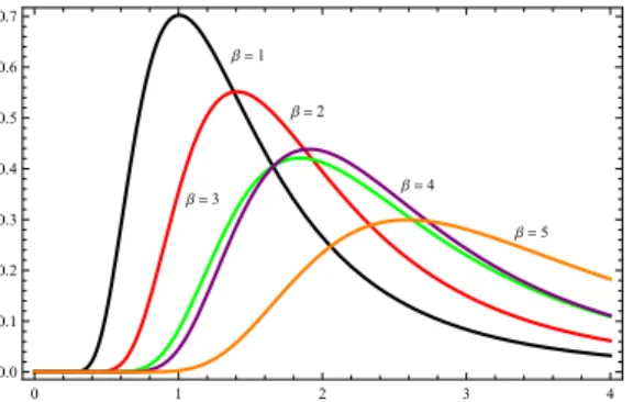
In Figure 2, we can clearly see that atγ = 3.5 function shows high peak, but as the value of γ are decreasing a rapid change appears it starts decreasing but no change appears in the location of the curve.
b =1
b =2
b =3 b =4
b =5
0 1 2 3 4
0.0 0.1 0.2 0.3 0.4 0.5 0.6 0.7
Figure 2: Graph for pdf ofT LIW forα= 2,γ= 1.5and for different values ofβ
g =3.5
g =3
g =2
g =1.5
g =1
0 1 2 3 4
0.0 0.5 1.0 1.5
Figure 3: Graph for pdf ofT LIW forα= 2,β= 2 and for different values ofγ
3. Properties of TLIW Distribution
In this section, we discuss important and useful statistical characteristics of the pro-posed distribution.
3.1. Quantile and Median
The qth percentile of the distribution can be obtained by solving yq for variable Y.
The qth percentile is obtained by solvingQ(y)=F(y)−1 as:
yq=−
β
ln[1−
q
1−qα1]
1 γ
, q >0. (10)
b =1
b =2
b =3
b =4 a =3
0.5 1.0 1.5 2.0 2.5 3.0 0.2 0.4 0.6 0.8 1.0 b =2 b =1 b =4 b =3
a =2
0.5 1.0 1.5 2.0 2.5 3.0 0.2 0.4 0.6 0.8 1.0 1.2 b =1 b =2 b =3 b =4 a =1.5
0.5 1.0 1.5 2.0 2.5 3.0 0.2 0.4 0.6 0.8 1.0 1.2
b =0.5
b =1
b =1.5
b =2 a =0.5
0.5 1.0 1.5 2.0 2.5 3.0 0.5
1.0 1.5
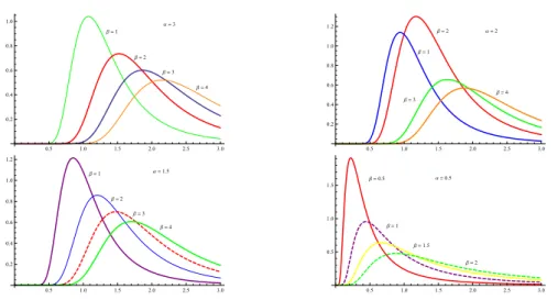
Figure 4: Graph for pdf ofT LIW forα= 0.5,1.5,2,3andβ= 1,2,3,4andγ= 2
3.2. Moments
The moments of Topp-Leone Inverse Weibull distribution is computed using following expression
µ0r =
Z ∞
0
yrF(y)dy=
Z ∞ 0 yr ∞ X j=0 2j+1
X
m=0
(−1)j+m2Γ(α+ 1)
j!Γ(α−j)
2j+ 1
m
βγ yγ+1{e
−β
yγ
}m+1dy.
(11)
Making transformation as z= (m+1)yr β in above expression to solve the moment of Topp-Leone Inverse Weibull distribution and result are given as follows
µ0r=
∞ X
j=0 2j+1
X
m=0
(−1)j+m2Γ(α+ 1)
j!Γ(α−j)
2j+ 1
m
1
β(m+ 1)
1−r
γ
Γ(1− r
γ). (12)
These moments are existing for r < γ. The coefficient of variation (CV), coefficient of skewness (CS) and coefficient of kurtosis (CK)T LIW distribution are obtained as follows
CV =
rµ 2
µ1
−1.
CS= µ3−3µ2µ1+ 2µ 3 1
(µ2−µ1) 3 2
.
CK = µ4−4µ3µ1+ 6µ2µ 2 1 (µ2−µ21)2
3.3. Reliability Analysis
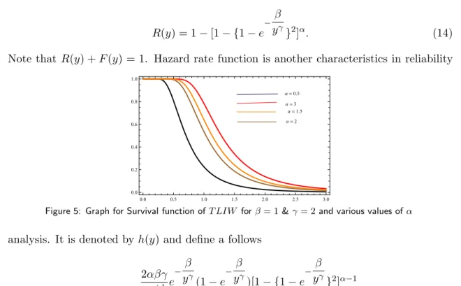
TheT LIW distribution is used for describing a random lifetime in reliability analysis. The reliability analysis of the T LIW distribution is denoted by R(y), also known as survival function and obtained as follows
R(y) = 1−F(y). (13)
The survival function of T LIW distribution is obtained by inserting (5) in to above ex-pression (15) to attain the following results
R(y) = 1−[1− {1−e
−β
yγ
}2]α. (14)
Note that R(y) +F(y) = 1. Hazard rate function is another characteristics in reliability
a =0.5
a =3
a =2 a =1.5
0.0 0.5 1.0 1.5 2.0 2.5 3.0
0.0 0.2 0.4 0.6 0.8 1.0
Figure 5: Graph for Survival function ofT LIW forβ= 1&γ= 2 and various values ofα
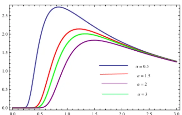
analysis. It is denoted by h(y) and define a follows
h(y) = 2αβγ
yγ+1 e −β
yγ
(1−e
−β
yγ
)[1− {1−e
−β
yγ
}2]α−1
1−[1− {1−e
−β
yγ
}2]α
(15)
The units for h(y) is the probability of failure per unit of distance and time. We define these failure rates at the different values of parameters. The cumulative hazard rate function of T LIW distribution is represented as H(y) and the result obtained are given as follows
h(y) =−log|1−[1− {1−e
−β
yγ
}2]α|. (16)
a =0.5
a =1.5
a =2
a =3
0.0 0.5 1.0 1.5 2.0 2.5 3.0
0.0 0.5 1.0 1.5 2.0 2.5
Figure 6: Graph for Hazard rate function ofT LIW forβ= 1&γ= 2and various values ofα
3.4. Mode
We consider the density function ofT LIW distribution given in (6) and solve ∂ln∂yf(y) = 0 for y, to obtain the mode of Topp-Leone Inverse Weibull distribution as follows
∂lnf(y)
∂y =
βγ
y −
e−βy−γy−(1+γ)βγ
1−e−βy−γ +
2e−βy−γ(1−e−βy−γ)y−(1+γ)βγ
1(1−e−βy−γ
)2 +
1 +γ
y .
By putting ∂ln∂yf(y) = 0, we have:
βγ
y −
e−βy−γy−(1+γ)βγ
1−e−βy−γ +
2e−βy−γ(1−e−βy−γ)y−(1+γ)βγ
1(1−e−βy−γ
)2 +
1 +γ
y = 0 (17)
The maxima can be obtained by solving (17) iteratively.
4. Order Statistics
Order statistics is used in the field of reliability and life testing widely. LetX1, X2, ... , Xn
be a simple random sample from T LIW(α, β, γ) with distribution and density functions given in (5) and (6). Let X(1:n) ≤ X(2:n)l... ≤ X(n:n) denote the order statistics ob-tained from this sample. In reliability literature, X(j:n) is used to model the lifetime of an (ni+ 1)-out-of-n system which consists of n independent and identically distributed components. The density function ofX(i:n), 1≤k≤nis given as follows:
fi,n(x) =
n!
(i−1)!(n−i)![FEGW E(x)]
i−1[1−F
EGW E(x)]n−ifEGW E(x)
The first order statistic is given byX(1) =min(X1, X2, ...Xn) and the last order statistics
is given by X(n) =max(X1, X2, ...Xn). The distribution of first order statistics is given
by
f1:n(y) = 2nαβγ
∞ X
j=0
(−1)j Γ(n)
j!Γ(n−j)[1−(1−e
−yγβ
)2]αj+α−1y−(γ+1)e−
β
yγ(1−e− β yγ).
The distribution of the nthorder statistics is given by
fn:n(y) = 2nαβγy−(γ+1)e
−β
yγ(1−e− β
yγ)[1−(1−e− β
yγ)2]n+α−2 (19)
5. Parameters Estimation and Fisher Information Matrix
In this section, we derive the maximum likelihood estimates (MLE) and inference for unknown parameters of Topp-Leone Inverse Weibull distribution. Let y1, y2...yn be
a realization of a random sample of size n from T LIW distribution than the likelihood function is written as follows
LF =L(α, β, γ|yi) = n
Y
i=0
F(yi),
the log-likelihood function is given as follows
ln(LF) =nln(2) +nln(α) +nln(β) +nln(γ)−(γ+ 1)
n
X
j=1
ln(yj)−β n
X
j=1
ln(y−jγ)+
n
X
j=1
ln(1−e
−β
yγ
j) + (α−1)
n
X
j=1
ln(1− {1−e
−β
yγ
j}2), (20)
differentiating (22) w.r.tα, β,γ, and equating them 0, we have
n α +
n
X
j=1
ln 1−w2= 0, (21)
n β +
n
X
j=1
yj−γe
−β yγ j w − n X j=1
ln(y−jγ)−(α+ 1)
n
X
j=1
2yj−γ(w)e
−β
yγ j
1−w2 = 0, (22)
n γ +β
n
X
j=1
ln(yj)− n
X
j=1
ln(yj)− n
X
j=1
y−jγβln(yj)e
−β yγj
w +
(α+ 1)
n
X
j=1
2yj−γβln(yj)we
−β
yγ j
1−w2 = 0, (23)
where (1−e
−β
yjγ
) = w. The maximum likelihood estimate of α, β, and γ are obtained iteratively solving (21), (22), and (23), simultaneously. The fisher information matrix for the parameters of the T LIW distribution is obtained as follows
ˆ α ˆ β ˆ γ
∼N α β γ . ˆ
Jαα Jˆαβ Jˆαγ
ˆ
Jββ Jˆβγ
1
J =−E
Jαα Jαβ Jαγ
Jββ Jβγ
Jγγ
.
By determining the inverse dispersion matrix, the asymptotic variances and covariances of the ML estimators forα, β,andγmay be obtained. Using above, approximate 100(1−λ)% confidence intervals for α, β, andγ are determined respectively as follows
ˆ
α±Z λ
2
q
ˆ
Jαα, βˆ±Z λ
2
q
ˆ
Jββ, γˆ±Z λ
2
q
ˆ
Jγγ, (24)
whereZγ is demonstrated the upper 100γth quantile of the standard normal distribution.
6. Simulation Study
In this section of article, we discuss some simulations for different sample size to de-termine the efficiency of MLEs. The different methods have been derived for simulating a random variable like the inversion method, the rejection, acceptance sampling techniques, and many more from different probability distributions in the field of computational statis-tics. The Inversion method is considered the most powerful technique. We can simulate random variableY given by
y=−
β
ln[1−
q
1−U1α]
1 γ
,
whereU is uniform random number in (0,1). We generate sample of sizen= 50,100,200,500,
1000 from T LIW distribution for some selected combination of parameters. This process is repeatedN = 1000 time to calculate mean estimate and means squared error. Obtained results are given in following tables.
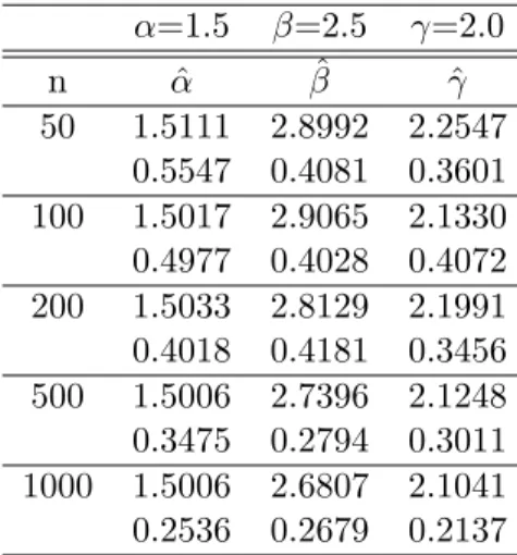
It is observed that when sample size increases the mean squared error decreases. There-fore, the maximum likelihood method works very well to estimate the parameters ofT LIW
distribution.
7. Application
Table 1: Estimated Mean and MSEs of TLIW distribution
α=2.5 β=2.0 γ=1.5
n αˆ βˆ γˆ
50 2.5073 2.0288 1.5741
0.6507 0.4327 0.3810
100 2.5033 2.0118 1.8671
0.3684 0.4463 0.3544
200 2.5018 2.1605 1.8339
0.3582 0.3758 0.3673
500 2.5014 2.3003 1.7115
0.2661 0.3688 0.3637 1000 2.5009 2.0421 1.9818 0.2373 0.2884 0.2906
Table 2: Estimated Mean and MSEs of TLIW distribution
α=1.5 β=2.5 γ=2.0
n αˆ βˆ γˆ
50 1.5111 2.8992 2.2547
0.5547 0.4081 0.3601
100 1.5017 2.9065 2.1330
0.4977 0.4028 0.4072
200 1.5033 2.8129 2.1991
0.4018 0.4181 0.3456
500 1.5006 2.7396 2.1248
0.3475 0.2794 0.3011 1000 1.5006 2.6807 2.1041 0.2536 0.2679 0.2137
Data Set 1:
For getting the performance of the proposed model a data related to influence of physiographic and historical factors on species richness of native and non-native vascular plants on 22 coastal islands is selected. Different variables are effecting on the richness. We select variable area (hectares) having values 3, 4, 4, 8, 10, 34, 40, 46, 47, 61, 128, 140, 350, 1190, 1350, 1900, 2300, 2707, 10900, 13600, 13600 and 26668.
It is depicted from the results of Table 7 that our proposed model provide best fit than recent developed models. It is be more reliable with these types of data.
From Figure. 7, we see that the data provides best fitting for proposed distribution.
Data Set 2:
Table 3: Parameter Estimation for Various Distributions
Model parameters LL
α β γ
T LIW 4.597689 0.4233699 0.20622405 -73.86899
EE 0.328589 0.02146033 -76.14519
EW 2.07528 1.533359 0.2841065 -96.15165
IE 4.597689 0.42333699 -249.7032
Figure 7: Goodness of Fit
12, 1998 by Jim Irish and has been referenced by several authors including da Silva, Thiago, Maciel, Campos and Cordeiro [8] and Pinho, Cordeiro and Nobre [9]. The actual data are: 83, 51, 87, 60, 28, 95, 8, 27, 15, 10, 18, 16, 29, 54, 91, 8, 17, 55, 10, 35, 47, 77, 36, 17, 21, 36, 18, 40, 10, 7, 34, 27, 28, 56, 8, 25, 68, 146, 89, 18, 73, 69, 9, 37, 10, 82, 29, 8, 60, 61, 61, 18, 169, 25, 8, 26, 11, 83, 11, 42, 17, 14, 9, 12.
Table 4: Parameter Estimation for Various Distributions
Model parameters LL
α β γ
T LIW 4.597689 0.4233699 0.2062405 -54.82303
EW 2.075585 1.532594 0.291697 -166.880
In Table 8, the value of log-likelihood ofT LIW distribution is minimum than other existing distributions, which indicates that new model is better.
The data of waiting time of customers are also provides better fit to follow the curve.
8. Conclusion
Figure 8: Goodness of Fit
References
[1] A. Al-Shomrani, O. Arif, A. Shawky, S. Hanif and M.Q. Shahbaz. Topp leone family of distributions: Some properties and application, Pakistan Journal ofStatistics and Operation Research.12(3):443-451, 2016.
[2] A.K. Gupta and S. Nadarajah . Handbook of Beta Distribution and its Applications. New York: Marcel Dekker Inc, 2004.
[3] A.P. Prudnikov, Y.A. Brychkov and O.I. Marichev.Integrals and Series. Vol. 3. New York: Gordon and Breach Science Publishers, 1986.
[4] A.Z. Keller and A.R.R. Kanath. Alternative reliability models for mechanical systems. Third Int. Conf. Reliab. Maintainabil.Toulse, France, pp. 411415, 1982.
[5] C. Lee, F. Famoye and O. Olumolade. Beta-Weibull distribution: some properties and applications to censored data.Journal of modern applied statistical methods.6(1):17, 2007.
[6] E. L. Lehmann. The power of rank tests.Annals of Mathematical Statistics.24:23-43, 1953.
[7] G.M. Cordeiro, E.M.M. Ortega and D.C.C. da Cunha. The exponentiated generalized class of distributions.J. of Data Science 11:127, 2013.
[8] G.R. Aryal, E.M. Ortega, G. Hamedani, and H.M. Yousof. The Topp-Leone Gen-erated Weibull Distribution: Regression Model, Characterizations and Applications. International Journal of Statistics and Probability.6:126, 2016.
[9] L.G. Pinho, G.M. Cordeiro and J.S. Nobre. The Harris extended exponential distri-bution.Communications in Statistics- Theory and methods.44:3486-3502, 2015.
[11] M. Aleem and G.R. Pasha. Ratio, product and single moments of order statistics form Inverse Weibull distribution.J. Statist.10(1):708, 2003.
[12] M. Aleem. Product, ratio and single moments of lower record values of inverseweibull distribution.J. Statist. 12(1):23-29, 2005.
[13] M.Q. Shahbaz, S. Saman and N.S. Butt. The Kumaraswamy Inverse Weibull Distri-bution.PJSOR. Vol. 3:479-489, 2012.
[14] M.V. Aarset. How to identify bathtub hazard rate. IEEE Transactions Reliability. 36:106-108, 1087.
[15] N.L. Johnson and S. Kotz. Continuous Univariate Distributions. Vol. 1. New York: John Wiley and Sons, 1970.
[16] R. Calabria and G. Pulcini. On the maximum likelihood and least-squares estimation in the Inverse Weibull distributions.Statist. Appl.2(1):53-66, 1990.
[17] R. Calabria and G. Pulcini. Bayes 2-sample prediction for the Inverse Weibull distri-bution.Commun. Statist. Theor. Meth. 23(6):1811-1824, 1994.
[18] R.D. Gupta and D. Kundu. Generalized exponential distribution. Aust. N.Z.J. Stat. 41:173-183, 1999.
[19] R.D. Gupta and D. Kundu. Generalized exponential distribution: different methods of estimations. j. Stat. Comput. Sim.69:315-338, 2001.
[20] R. da Silva, A. Thiago, D. Maciel, R. Campos, and G. Cordeiro. A new lifetime model: the gamma extended Frechet distribution. Journal of Statistical Theory and Applications.12:39-54, 2013.
[21] S. Hanook, M.Q. Shahbaz, M. Mohsin and B.M.G. Kibria. A Note On Beta Inverse Weibull distribution.Comm.Statict.Theor.Meth. 42:320-335, 2013.
[22] S. Nadarajah and S. Kotz. The beta exponential distribution Reliability engineering & system safety,Elsevier. 91:689-697, 2006.
[23] W. Nelson. Applied Life Data Analysis New York. John Wiley and Sons New York. 1982.
Table 5: Mean of Toop-Leone Inverse Weibull distribution for different values of parameters
β
α γ 4 5 6 7 8 9
1 1 0.125 0.221556731 0.281270921 0.320461669 0.347920893 0.368165662
1 2 0.08 0.158533092 0.208887035 0.242459148 0.266188013 0.283779878
1 3 0.055555556 0.120600209 0.163808521 0.193046537 0.213880406 0.229405316 1 4 0.040816327 0.095703512 0.133374899 0.159213001 0.177760331 0.191645616
1 5 0.03125 0.078332134 0.111622439 0.134737534 0.151441365 0.163999158
1 6 0.024691358 0.065646439 0.095399949 0.116291492 0.131480543 0.142943258
2 1 0.097222222 0.228051309 0.316474846 0.376617996 0.419571752 0.45161973
2 2 0.062222222 0.163180233 0.235031378 0.284946648 0.321006795 0.348105772 2 3 0.043209877 0.124135409 0.184310829 0.226875184 0.257926955 0.281405839 2 4 0.031746032 0.098508906 0.150068128 0.187112804 0.214368309 0.235086947 2 5 0.024305556 0.080628313 0.125593126 0.158348361 0.182629212 0.201173719
2 6 0.01920439 0.067570758 0.107340226 0.136669914 0.158557657 0.175344966
3 1 0.087916667 0.238778166 0.347213665 0.422774371 0.477437645 0.518548753 3 2 0.056266667 0.170855748 0.257859691 0.319868251 0.365278948 0.399694261 3 3 0.039074074 0.129974371 0.202212717 0.254679846 0.293499353 0.323109548 3 4 0.028707483 0.103142473 0.164644064 0.210044392 0.243933249 0.269926302
3 5 0.021979167 0.08442083 0.137791834 0.177754726 0.207816806 0.23098721
3 5 0.017366255 0.070749086 0.117766053 0.153419479 0.180425384 0.201330694 4 1 0.083129252 0.248977245 0.373566076 0.461917367 0.526433444 0.575236864
4 2 0.053202721 0.178153614 0.27743042 0.349483579 0.402764752 0.443389116
4 3 0.036946334 0.135526046 0.217560017 0.278259639 0.323618963 0.358432109 4 4 0.027144245 0.107548061 0.177140024 0.229491566 0.268966266 0.299434833 4 5 0.020782313 0.088026749 0.148249795 0.194212329 0.229143466 0.256238892 4 6 0.016420593 0.073771036 0.126704121 0.167623978 0.198941071 0.223340305
5 1 0.080157943 0.258247777 0.39666873 0.496177192 0.569372114 0.624992261
5 2 0.051301083 0.184787067 0.294587704 0.375404333 0.435616356 0.481740277 5 3 0.035625752 0.140572285 0.231014702 0.298897803 0.350015021 0.389434872 5 4 0.026174022 0.111552554 0.188094993 0.246512665 0.290904564 0.325334597
5 5 0.020039486 0.091304377 0.15741809 0.208616811 0.247833607 0.278402402
5 6 0.015833668 0.07651786 0.134539954 0.180056436 0.215167746 0.242658235
6 1 0.078108153 0.26666609 0.417325949 0.526846126 0.607887428 0.669699166
6 2 0.049989218 0.190810721 0.309928874 0.398608242 0.465083729 0.51620009
6 3 0.034714735 0.145154634 0.243045198 0.31737281 0.373691871 0.417291901
6 4 0.025504703 0.115188924 0.197890369 0.261749722 0.310582873 0.34860641
6 5 0.019527038 0.0942807 0.165615913 0.221511509 0.264598371 0.298317064
Table 6: Variance of Toop-Leone Inverse Weibull distribution for different values of parameters
β
α γ 4 5 6 7 8 9
1 1 0.001953125 0.004661601 0.005216654 0.004891093 0.004335786 0.003775348
1 2 0.001152 0.003083723 0.003646001 0.003521791 0.003180363 0.002804469
1 3 0.000685871 0.002115403 0.002640853 0.002624235 0.002411365 0.00215147
1 4 0.000424993 0.001506302 0.001977551 0.002016728 0.001882668 0.001697738
1 5 0.000274658 0.001108364 0.001523567 0.001590785 0.001506476 0.00137166
1 6 0.000184404 0.000838659 0.001202209 0.001282461 0.00123043 0.001130183
2 1 0.002492311 0.008558125 0.010981446 0.01103603 0.010200011 0.00913207
2 2 0.00118062 0.00509626 0.007082722 0.00741353 0.007023159 0.006392909
2 3 0.000623835 0.003274471 0.004870687 0.005277731 0.00510592 0.00471372
2 4 0.000358556 0.002228641 0.003515642 0.003925325 0.003867254 0.0036141
2 5 0.000220038 0.001586127 0.002634618 0.003020203 0.003023556 0.002856213
2 6 0.000142254 0.001169653 0.002034192 0.002387347 0.00242439 0.002312322
3 1 0.002475099 0.011379596 0.016066296 0.016927302 0.016091374 0.014677856
3 2 0.001117531 0.006565329 0.010091408 0.011102363 0.010834666 0.010058523
3 3 0.000573636 0.004131432 0.006816692 0.007775728 0.007756672 0.007308022
3 4 0.000323372 0.002770284 0.004856429 0.00571401 0.005808386 0.005542175
3 5 0.000195709 0.001949481 0.003603018 0.004355608 0.004501103 0.004342689
3 6 0.000125211 0.001424863 0.002759653 0.003417197 0.003583404 0.003491525
4 1 0.002426513 0.013752778 0.02079772 0.022671748 0.021994874 0.020335553
4 2 0.001072231 0.007806363 0.012879095 0.014676978 0.014627679 0.013771144
4 3 0.000543067 0.00485898 0.008615332 0.010186439 0.010382128 0.009922473
4 4 0.000303361 0.003232387 0.00609377 0.007435109 0.007724326 0.00747801
4 5 0.000182388 0.002260907 0.004495791 0.005637689 0.00595556 0.005830823
4 6 0.000116105 0.001644537 0.003427988 0.004404187 0.00472185 0.004669276
5 1 0.002383433 0.015857995 0.02528833 0.028305203 0.027897746 0.026065817
5 2 0.001040135 0.008909254 0.015516512 0.018167471 0.018402466 0.017513043
5 3 0.000522688 0.005506887 0.010313572 0.012533485 0.012986384 0.012548475
5 4 0.000290405 0.003644747 0.007260406 0.009107116 0.00962012 0.009417354
5 5 0.000173912 0.002539342 0.005336683 0.006881104 0.007391947 0.007318602
5 6 0.000110377 0.001841286 0.004056991 0.005360118 0.00584439 0.005844781
6 1 0.0023482 0.017777048 0.029595667 0.033846826 0.033792679 0.03184612
6 2 0.001016344 0.009915348 0.018039936 0.021589905 0.022158922 0.021273907
6 3 0.000508067 0.006098486 0.011935698 0.01482955 0.015571548 0.015180957
6 4 0.000281262 0.00402163 0.008373418 0.010740034 0.011498479 0.011357662
6 5 0.000167991 0.002794055 0.006138195 0.008093839 0.008813009 0.008804798
Table 7: Coefficient Skewness Table of Toop-Leone Inverse Weibull distribution for different values of parameters
β
α γ 4 5 6 7 8 9
1 1 0.595170064 0.44020366 0.355459867 0.296998208 0.254493126 0.222361967
1 2 0.582377652 0.458810019 0.373560513 0.312841916 0.26825751 0.234420311
1 3 0.595170064 0.47859545 0.391051237 0.327786601 0.281104898 0.245608469
1 4 0.611011148 0.496551293 0.406805639 0.341251432 0.292686152 0.25569677
1 5 0.625259785 0.512279767 0.420789994 0.353286558 0.303076239 0.264766849
1 6 0.63718253 0.525966374 0.433203744 0.364068159 0.312429005 0.272954236
2 1 0.61181318 0.491730312 0.399990748 0.334114492 0.285803679 0.249242975
2 2 0.636540479 0.519239851 0.424383364 0.355018962 0.303788457 0.264901376 2 3 0.653449639 0.540633294 0.444183098 0.372308778 0.318809681 0.278054474 2 4 0.665160849 0.557618288 0.460579618 0.386891791 0.331601108 0.289318072 2 5 0.673507548 0.571399058 0.474418518 0.399413524 0.342683707 0.299128606
2 6 0.679630911 0.582797364 0.48629096 0.410328964 0.352425876 0.307795142
3 1 0.64455463 0.525932188 0.42920009 0.358551554 0.306481958 0.267030449
3 2 0.663187691 0.551736925 0.453570335 0.379982246 0.32515735 0.283407843
3 3 0.674746479 0.570998667 0.472801624 0.397306103 0.340444782 0.296913327
3 4 0.682333473 0.585910543 0.488451014 0.41171273 0.353303161 0.308348995
3 5 0.687557619 0.597799548 0.501499074 0.423962495 0.364349609 0.318232934 3 6 0.691298849 0.607505692 0.512591088 0.434563263 0.373999243 0.326915003 4 1 0.661850384 0.547910128 0.449100662 0.375623929 0.321119419 0.279720092
4 2 0.6760347 0.571771624 0.472867786 0.396987389 0.339943143 0.296332247
4 3 0.684527968 0.589268286 0.491389767 0.414082734 0.355216045 0.309920793 4 4 0.689984409 0.602654923 0.506337079 0.428204846 0.367988327 0.321366816
4 5 0.693687521 0.613237061 0.518724385 0.440154911 0.37891557 0.331223044
4 6 0.696311928 0.621819793 0.529205403 0.450458034 0.388431041 0.339856478
5 1 0.672058453 0.563383103 0.463827394 0.388529415 0.332308138 0.2894842
5 2 0.683344122 0.585604157 0.486944539 0.409687845 0.351123296 0.306176831
5 3 0.689975891 0.601727657 0.504826258 0.426517997 0.366310149 0.31976694
5 4 0.694186506 0.613975473 0.519183129 0.440364459 0.378966181 0.331178398 5 5 0.697021075 0.623606163 0.531035751 0.452045938 0.389766266 0.340982479 5 6 0.699018113 0.631385074 0.541034307 0.462093722 0.399152327 0.349555166 6 1 0.678684577 0.575005194 0.475356676 0.398813552 0.341307364 0.297380969
6 2 0.687993054 0.595871432 0.497868403 0.419734508 0.360056827 0.31409033
6 3 0.69339867 0.610904142 0.51519317 0.436308022 0.375137626 0.327651048
6 4 0.696805022 0.622266808 0.529053126 0.449904702 0.387674997 0.339013353
6 5 0.699086216 0.631168414 0.540464558 0.461351002 0.39835462 0.34875972
Table 8: Coefficient Kurtosis Table of Toop-Leone Inverse Weibull distribution for different values of parameters
β
α γ 4 5 6 7 8 9
1 1 2.21799308 1.966578604 1.862381523 1.80009056 1.760174038 1.73327196
1 2 2.16901906 1.989904972 1.883432354 1.816402864 1.772737797 1.74310779
1 3 2.181110946 2.016869168 1.90481036 1.832527085 1.785022917 1.752667989
1 4 2.202955207 2.042152468 1.924734817 1.847602602 1.796534824 1.761637457 1 5 2.223602742 2.064704401 1.942880501 1.861487726 1.807202265 1.769977724
1 6 2.24096953 2.084540107 1.959311759 1.874237491 1.817070246 1.777725965
2 1 2.204489811 2.036104942 1.916580368 1.839858533 1.78981241 1.755946971
2 2 2.240606729 2.075608857 1.94820648 1.863880822 1.808153183 1.770216939
2 3 2.264802891 2.10672518 1.974688289 1.884564185 1.824177496 1.782790477
2 4 2.281082808 2.131525557 1.997085128 1.902538595 1.838305036 1.79396941
2 5 2.29236257 2.151632244 2.016268719 1.918330963 1.850887744 1.804006191
2 6 2.300429861 2.168208738 2.032900341 1.932349445 1.862200357 1.813098363 3 1 2.252468424 2.085733006 1.954876814 1.868222783 1.811079219 1.772270322 3 2 2.278579891 2.123307968 1.987756083 1.894151879 1.831246757 1.788122103 3 3 2.294145059 2.151374944 2.014300699 1.915844774 1.848442191 1.801788923
3 4 2.304018064 2.173008331 2.036215819 1.934338592 1.863357444 1.81376549
3 5 2.310626055 2.190142298 2.054660701 1.95036039 1.876483991 1.824405257
3 6 2.315248396 2.204025169 2.070437485 1.964427808 1.888176302 1.833964757
4 1 2.276880262 2.11795912 1.981834288 1.888905862 1.826872113 1.784520163
4 2 2.295923215 2.152696196 2.014564254 1.91555608 1.847940813 1.801233494
4 3 2.306864739 2.178027155 2.040520928 1.937535073 1.865686459 1.815487319
4 4 2.313668839 2.197244192 2.061686867 1.956085192 1.88094743 1.827883598
4 5 2.318168782 2.212292909 2.079337196 1.972033938 1.894291198 1.838833043 4 6 2.321292188 2.224382876 2.094325414 1.985952959 1.906115698 1.848625904
5 1 2.290740331 2.140641649 2.00214852 1.904969444 1.83933291 1.794274901
5 2 2.305401566 2.172858021 2.034373807 1.931912495 1.86092724 1.811540645
5 3 2.313681404 2.196018321 2.059645978 1.953931371 1.878974432 1.826163993 5 4 2.318782032 2.213421623 2.080091359 1.972393941 1.894407978 1.838818611 5 5 2.322136141 2.226956821 2.097039316 1.988188021 1.907844608 1.849953668 5 6 2.324455544 2.237774744 2.111363531 2.001916881 1.919710249 1.859882055 6 1 2.299464409 2.157619068 2.018233649 1.918014776 1.849588667 1.802366837
6 2 2.311255591 2.187713111 2.049862918 1.945056629 1.871517707 1.82001981
6 3 2.317850054 2.209140615 2.074472692 1.967012738 1.889742551 1.834897154
6 4 2.321890778 2.22513783 2.094270298 1.985335727 1.905264668 1.847725164