An Extended Model for Multi-Criteria Software Component Allocation on a Heterogeneous Embedded Platform

An Extended Model for Multi-Criteria

Software Component Allocation on a

Heterogeneous Embedded Platform

Ivan

Svogor

ˇ

_{, Ivica Crnkovi´c}

_{and Neven Vr}

_cek

_ˇ

1_{Faculty of Organization and Informatics, University of Zagreb, Croatia} 2_{School of Innovation, Design and Engineering, M¨alardalen University, Sweden}

A recent development of heterogeneous platforms(i.e. those containing different types of computational units such as multicore CPUs, GPUs, and FPGAs)has enabled significant improvements in performance for real-time data processing. This potential, however, is still not fully utilized due to the lack of methods for optimal config-uration of software; the allocation of different software components to different computational unit types is cru-cial for getting the maximal utilization of the platform, but for more complex systems it is difficult to find ad-hoc a good enough or the best configuration. With respect to system and user defined constraints, in this paper we are applying analytical hierarchical process and a genetic algorithm to find feasible, locally optimal solution for allocating software components to computational units.

Keywords: software, component, allocation, genetic al-gorithm, AHP, optimization, model, multi-criteria, em-bedded system

1. Introduction

The computer systems today are becoming het-erogeneous; alongside multicore Central Pro-cessing Units(CPU), Graphical Processing Units (GPU) and Field Programmable Gate Array (FPGA)are gaining an important role[1]. Such systems consist of different types of comput-ing units, where each unit can be dedicated to a particular type of computation. Using dif-ferent computational units is already a proved approach in high performance computer sys-tems, in which GPUs process highly parallel computation, and in which cores from multi-core CPUs perform different tasks in parallel. This is also becoming of significant importance

in embedded systems where such systems en-able processing of large amount of data streams in real time. This great potential for increased performance is still not fully utilized due to the lack of software methods for an efficient and op-timal placement(allocation)of software to the heterogeneous platform by which an optimal, or sufficiently good performance is obtained. Different software allocations result with dif-ferent performance and it is not obvious which allocation would enable the best performance. In addition, best allocation candidate might not be allowed due to different constraints; this can be due to limitation of resources of a particular unit(such as memory or communication capac-ity, or restricted energy consumption₎, or due to some architectural decisions related to spe-cific requirements ₍such as a requirement that two components are not allowed to be allocated to the same physical computational unit₎. A “trial and error” method by repeated allocations and then measurements is an inefficient proce-dure, in particular when the software implemen-tation may depend on which compuimplemen-tational unit type will be executed. For this reason, alloca-tion method is desired in an early development phase.

We assume that we are dealing with component-based systems, so each software component1 can be allocated to a computational unit. We define a method for finding an optimal alloca-tion of components in respect to optimal perfor-mance and different constraints. The method is assumed to be used in an early phase of the development lifecycle, in the early architectural design of the system. The components may already be implemented, or we can use their models. In the latter case the components may not be yet implemented, but are specified with a set of attributes, estimated or obtained in a cer-tain way. Current model abstraction level does not consider dependencies which might arise from operating system level. Also, at this stage we are considering cross platform communica-tion, i.e. that between components allocated on different computational units. Internal commu-nication between cores in multicore CPUs is not so influential on the rest of the system(more on this can be found in[18]). Similar assumption applies to GPU. Therefore, we focus only on components and their interaction, the result of the method is a proposed system deployment configuration that is optimal, or nearly optimal, for the overall system performance.

The rest of the paper is organized as follows. In the second chapter we define the problem and its formal description. In the third chapter we present our solution for the allocation problem using genetic algorithm. Chapter 4 describes method for finding optimal solution. Chapter 5 illustrates the model on an Autonomous Un-derwater Vehicle Case Study. Chapter 6 briefly discusses the related work, and finally Chapter 7 concludes the paper.

2. Component Allocation Method

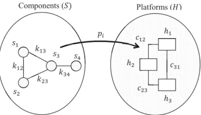
We define a model which consists of a Software System S as a set of components, and a Hard-ware PlatformHas a set of computational units, as shown in Figure 1.

Every componentsi ∈ S,i = 0, . . . ,n needs to

be allocated to a computational unithi ∈H,i=

0, . . . ,m. From a mathematical viewpoint, the problem is reduced to finding a permutation

(with repetition) which provides the best per-formance considering a set of defined resources and constraints of a particular system. The num-ber of all possible solutions, i.e. allocations of components to computational units ismn_.

Ob-viously, the search space increases rapidly with the number of the components and computa-tional units, so to find the optimal component allocation with respect to a particular goal is (at least₎very time-consuming if the process is performed manually. For this reason we provide a theoretical model for finding an optimal ₍or locally optimal)allocation with respect to a par-ticular set of system and component properties for given characteristics of the software system, components and the hardware platform.

Components (ܵሻ Platforms (ܪሻ

݌௜ ݄ଵ

݄ଶ

݄ଷ ݏଵ

ݏଶ

ݏଷ ݏସ ݇ଵଶ

݇ଵଷ

݇ଶଷ ݇ଷସ

ܿଵଶ

ܿଶଷ

ܿଷଵ

Figure 1. Software components allocation to heterogeneous hardware platform.

Our model is defined as follows.

1. A computational unit provides a set of re-sources for the components being executed on it, e.g. CPU power, or available memory. The capacity, i.e. the amount of the resources of each computational unit must satisfy the needs of the components executed on that unit.

2. We enable allocation of the components to the computational units, and try to find their optimal distribution with respect to cost func-tion. In this case our cost function is the overall performance of a certain allocation. The model also takes some assumptions: 1. The system is built of a set of components

which are characterized as atomic computa-tional and deployable units(i.e. a component cannot be distributed over several computa-tional units).

2. Component allocation has the property of isomorphism (i.e. each component can be deployed on every computational unit₎. 3. The system can be exposed by a set of

con-straints, which specifies whether a particular component is supposed to be₍or not to be₎ mapped to a particular computational unit.

2.1. Elements of the model – definitions

This section presents a formal specification of information necessary for making a component allocation decision.

A component can be allocated on any computa-tional unit(if not explicitly defined otherwise). Each component requires a certain amount of resources that should be provided by the com-putational unit. This amount depends on the computational unit on which the component is deployed. To specify the resources required for each component on each computational unit, we define a 3-dimensional matrix called Resource Consumption Matrix:

Definition 1. For n software components, m

computational units, and l different resources,

T = [tijk]₍n×m×l) is a Resource Consumption Matrix where tijkrepresents the necessary

amo-unt of k-th resource of the i-th software compo-nent allocated on the j-th computational unit.

With Resource Consumption Matrix we know the amount (quantity) of resources necessary for each component on each of the platforms. In addition, we need to define a new matrix which will specify a set of resources each com-putational unit can provide(e.g. total execution time, static memory, dynamic memory, energy etc.).

Since there are mcomputational units, and the Resource Consumption Matrix definesl resour-ces, the size of the new matrix, the computa-tional Unit Resource Matrix, ism×l.

Definition 2. R= [rjk](m×l)is a Computational

Unit Resource Matrix where rjkrepresents k-th

resource of a j-th computational unit.

With matricesT andRdefined, we know how much of some resource a certain component needs while allocated to any computational unit. Still, the provided information is insufficient to make a decision about the component allocation since we also need to consider communication. It can be realized between components within

the same computational unit, or among different computational units.

We recognize two different communication as-pects; software and hardware. From the soft-ware viewpoint we can talk about the intensity of communication between components. For instance, components handling data acquisition and data processing would have larger commu-nication intensity than a component which is responsible for task delegations.

We define a new matrix which contains infor-mation about the communication channel cost between computational units. This is due to het-erogeneous computational units, which can be connected via different types of communication channels₍e.g. Ethernet, CAN-bus, Wi-Fi, etc.₎ [10]. To specify the communication cost, we define the Platform Communication Cost Ma-trix:

Definition 3.C = [cij](m×m)is a Platform

Com-munication Cost Matrix where cij represents a

communication cost between i-th and j-th com-putational unit. For i₌ j, cij =0.

The communication is also limited by a physi-cal constraint – the bandwidth, which must be taken into consideration.

Definition 4. _{B = [}bij]m×mis a Bandwidth

Ma-trix where bijrepresents communication

band-width available between i-th and j-th computa-tional unit.

Cost of the total communication between the components does not only depend on the char-acteristics of the communication channels be-tween the platforms, but also on the commu-nication between components defined by com-ponents behavior; comcom-ponents which commu-nicate intensively between computational units with high communication cost will have a larger impact on overall performance than those com-municating sporadically with less data exchange. To express this constraint, we define the com-munication intensity matrix:

Definition 5. K = [kij](n×n) is a

Communi-cation Intensity Matrix where kij represents a

communication intensity between i-th and j-th software component.

If components i and j are not communicating, then kij = 0; also notice that K is symmetric

By the definitions(1-5)all necessary resources and constraints are defined. In order to find an allocation which satisfies the criteria of a partic-ular system, one should evaluate all allocations (i.e. all permutations₎ and find the allocation which provides desired performance. The set of all possible allocations (of components to computational units₎is defined as follows:

Definition 6. Function pi:S→H is a

Compo-nent Mapping Function where pi= (p1, . . . ,pn)

∈ P defines a particular allocation of compo-nents from S to computational units from H, with i=1, . . . ,mn_.

In order to make different allocations, i.e. so-lution vectors comparable and to get the opti-mal allocation with respect to the overall system performance, we need a mathematical model to evaluate every solution – a cost function, which is the subject of the following section.

Elements of vectorpirepresent one mapping of

a component to the computational units. The example below shows the case where number of components is equal to number of computa-tional units ₍n ₌ m₎, and every software com-ponent is allocated on only one computational unit. Thepositionin solution vector represents a component and itsvaluerepresents the com-putational unit on witch it is allocated. In real world, it is more often that there are more com-ponents than computational units, and therefore some computational unitsh will occur on sev-eral positions across the vectorpi.

h1, h2, . . . , hm

↑ ↑ ↑

pi = (s1, s2, . . . , sn)

(1)

2.2. The allocation cost function

Now we will define a mathematical model in the form of a cost function which evaluates an allo-cation. Therefore, providing a normalized value of resource usage costs. In addition, the prede-fined constraints could exclude some particular allocations. With the ability to compare alloca-tionspi, one can find the optimal one. In order

to create a cost function, we must consider: a) different system resources, b)communication, which is further explained in the following sub-sections.

System Resource Constraints

System Resource Constraints function,ressums up normalized values of all resources used by the components for a particular allocation con-figurationpi, and it is defined as follows:

res =

l

k=1

fk n

i=1

tipik (2)

where

f – element of a trade-off vectorF

t– element of a resource consumption matrixT

l– number of different resources for matrix_T

n– number of components

Equation 2 consists of two sums. The inner one calculates total costs of each resource for all components. There areldifferent resources and they are marked withk. The outer one sums up all l resources. Summing different costs is possible due to normalization of resources val-ues(more on this topic in Section 2.3). In addi-tion, for a particular system, particular proper-ties may be of a larger importance₍for example, energy consumption can be more important than system reliability: A solution to put two com-ponents on one computational unit can be better for energy consumption, but for reliability it can be better to allocate these two components on different computational units). For this reason we introduced a trade-off vector F = [f]l+1 which defines relative importance of each re-source cost.

Notice that vector is l+1 long, wherelis the number of resources considered. First l ele-ments of the vector are marked asfk, and they

are used for giving importance to resources de-fined with matrix_T. ₍l₊1₎-th element, marked asfc, is used for importance of communication

in the following section(Equation 4).

Resource constraints

Equation 2 provides a resource cost for any con-figurationpi. However, there are configurations

Resource constraint factor=1, which defines the feasibility of an allocation configuration.

=

0,ni=1lk=1

tipik

<lj=1rpij 1,ni=11k=1

tipik

≥lj=1rpij where

r – element of the computational unit resource matrix_R.

The multiplier  is used to remove unfeasible configurations; If the required resources exceed maximum available resources on a particular computational unit, we set  = 0, effectively disregarding the current allocation. In all other cases,  = 1, meaning the available resources are not exceeded by the required resources in the current allocationpi.

Now Equation 2 multiplied by the factorgives a cost for a feasible allocation configuration.

res=

_l

k=1

fk n

i=1

tipik

· (3)

Communication resources and constraints

In addition to the computational unit resources that have impact on the performance, we have resources related to the communication between the components. The communication costs are expressed bycom:

com₌

i≤j

kij·cpipj (4)

where

k – element of a communication intensity ma-trixK

c – element of a platform communication cost matrixC

b– element of the bandwidth matrix_B

The sum in Equation 4 handles communication channels between computational units and mul-tiplies the platform communication cost ( de-fined by matrixC)with the communication in-tensity (defined by matrix K). Communica-tion intensity relates to the data exchanged be-tween different software components, while the platform communication cost relates to physi-cal characteristics. This will vary depending on which computational unit a component is allo-cated.

Like before, we define a multiplier that pre-vents an allocation in which the required com-munication resources exceed the available band-width.

 = 0,

i≤j

kij·cpipj

<i≤jbpij 1,i≤j

kij·cpipj

≥i≤jbpij whereb– element of the bandwidth matrix_B. The final form of the communication resource cost function is defined as follows:

com₌

⎛

⎝fc

i≤j

kij·cpipj

⎞

⎠_{· (}5₎

where

fc– the communication trade-off factor(the last

element in vectorF).

Final form of the cost function

In order to get the complete model, Equation 3 and Equation 5 need to be joined in a cost func-tionw_{= (}res₊com_)··:

w=

⎛

⎝l

k=1

fk n

i=1

tipik+fc

i≤j

kij·cpipj

⎞

⎠_··

(6₎ To find the optimal component allocation, we need to compare all feasible solutions pi from

Pand select the one with the smallestw₍greater than 0).

As already mentioned, the problem is in the size of|P|=mn_{which is a very large number.}

Small increases in sets SandH cause enlarge-ment of search space, which is not searchable in a polynomial time.

2.3. Handling different measurement units

k1

k2 ...

kl+1

k1 k2 . . . kl+1

⎛ ⎜ ⎜ ⎝

1 m1,2 . . . m1,l+1

(m1,2)−1 1 . . . m2,l+1

... ... ... ...

(m1,l+1)−1 (m2,l+1)−1 . . . 1

⎞ ⎟ ⎟

⎠=Mc (7)

this problem, we use Analytic Hierarchy Pro-cess(AHP) [15], a commonly used method for complex multidimensional choices, alternatives and tradeoffs.

A great benefit of this method is disregarding measurement units. It uses trade-off weights which assess the importance of different deci-sion criteria. Since it also uses human subjective judgment, AHP provides a procedure to verify consistency of the decision model.

For the model we present here, one level of hierarchy(Figure 2)is sufficient and it consid-ers the importance of different resources. For importance of each resource, a trade-off vector

F is used as shown in Equation 6. Its values should be calculated using AHP. To determine

F, we first need to address the importance of all different resources, i.e. AHP criteria used in the allocation model. AHP criteria are given by the third dimension of matrixT.

W

pi pi pi

Goal

Criteria

Alternatives (allocation)

k2

k1 kl+l

. . .

. . .

f1 f2

f1+f2+...+fl+1 = 1

fl+1

Figure 2.Hierarchy for defining the criteria.

The first step in AHP is to perform a pairwise comparison of all AHP criteria and form the comparison matrixMc along with hierarchy of

the criteria. This is shown in Figure 2. The solution vector pi, is an input for each AHP

criterion.

Matrix Mc provides a pairwise comparison of

resources considered by the model. For com-parison, we are using a standard AHP scale (1

– equal importance, 3 – slightly favoring, 5 – strong favors, 7 – very strong favoring, 9 – ex-treme favors). For instance, if resource k1 is slightly more important than resourcek2, conse-quentlym1,2 =3, andk2compared tok1would give the reciprocal value,m2,1=1/3. Fori=j,

m=1.

The next step, according to AHP, is to calculate normalized principal Eigenvector and principal Eigenvalue. The largest Eigenvalue is called principal Eigenvalue (max). The

Eigenvec-tor that corresponds to principal Eigenvalue is called Principal Eigenvector(∗_{). The}

Princi-pal Eigenvector should also be normalized so that sum of all elements equals 1, and its values are vectorF.

The final step, before attributing the Eigenvec-tor with the created hierarchy is to verify consis-tency of the model. Since pairwise comparison matrix is created by a subjective human judg-ment, AHP deals with this by measuring the consistency of prioritization. As it may hap-pen that pairwise comparison is not done in a consistent way, consistency ratioCR should be

calculated. It is given asCR =CI/RI, whereCI

is Consistency index andRI is Random

consis-tency index.

CI is calculated as:

CI = max−(l+1)

l

Random consistency index is calculated by gen-erating comparison matrix with values₍1_/9_,1_/8_, . . . ,8_,9₎, more on this topic can be found in [16].

Finally, ifCRis less or equal to 10%, the

incon-sistency of pairwise comparison is acceptable. Since different system properties (matrix T,

hour). Hence, before the calculation, the input matrices T, R and C need to be normalized, so all the values are in range from 0 to 1. 1 represents a maximum available amount of a resource; it is found in matrix R. Now, the only factor to decide the importance of a certain system property is the trade-off vectorF.

2.4. Additional constraints – architectural decisions

To get the optimal solution, we need to find pi

which gives minimum result min(w)∀pi ∈ P

(Equation 6₎considering all the given platform constraints. As opposed to platform constraints, system architectural decisions can also be con-sidered as a constraint, which somewhat de-creases the search space. The solution vector

piis becoming partially definedpi∈ P, where

P _{⊂ P is the reduced search space with valid}

solutions. Architectural decisions are included in our allocation model as an additional con-straint.

There are two architectural decisions ( addi-tional constraints)which can be specified: 1. a particular component should beorshould

not be allocated on a particular computa-tional unit

2. a set of componentsshould beorshould not beallocated on the same computational unit

3. Evolving the Solution with Genetic Algorithm

In order to get an optimal solution, the goal is to minimize the cost function (w). Since it is not feasible to search the entire solution space (due to large number of variables₎, a heuristic (e.g. greedy algorithm₎or meta-heuristic₍e.g. genetic algorithm, particle swarm optimization, simulated annealing) is a good choice to find a semi-optimal solution. We have chosen Ge-netic Algorithm(GA)which is frequently used for solving optimization problems by mimick-ing the process of evolution. The evolution of the solution is done by crossover between differ-ent solutions, in our case allocations(genes)and mutation. Bad allocations are disregarded and

the good ones are reinforced. Since GA needs a comparison function, andwcan be used as one, GA is a favorable choice. Also, our compar-isons have shown that it provides very accurate solutions Figure 3. For the implementation we usedPythonandPyevolve library with the fol-lowing settings:

Generations 50 Mutation rate 0,05 Crossover rate 0,95 Population size 80

Selection algorithm Roulette wheel

Table 1.GA settings.

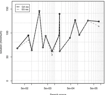
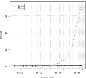
With the settings shown in Table 1, GA con-verges to the solution with average deviation of 3%. The exact solution was calculated by ex-haustive search(ES), which is a common tech-nique to systematically enumerate all solutions. Figure 3 shows the comparison between results of ES and GA. It is obvious that GA provides very accurate results. During the test of GA we also measured the execution time. Figure 4 shows that initially ES was faster, however with slow growth of inputs search space and time grew exponentially and GA was more efficient, as expected2_.

● ●

● ●

● ●

● ●

●

● ●

●

●

● _●

5e+02 5e+03 5e+04 5e+05

0

50

100

150

● ●

● ●

● ●

● ● ●

● ●

●

● ●

●

Search space

Solution (minim

um)

● ●

GA res ES res

Figure 3. Accuracy comparison between solutions from GA and EF(logarithmic scale).

● ● ● ● ● ● ● ●●● ● ● ● ● ●

5e+02 5e+03 5e+04 5e+05

02

0

4

0

6

0

● ● ● ● ● ● ● ●●●

● ● ●

● ●

Search space

Time (s)

●

●

GA res ES res

Figure 4. Execution time comparison for GA and EF search(logarithmic scale).

The application of Genetic Algorithm does not guarantee an optimal solution, however it will provide one which is sufficiently good, given the time necessary to calculate it. Here, we used GA simply to gain the solution faster, however at the cost of accuracy. For the purpose of the following use case, the accuracy was accept-able.

1 UI

2 CH

3 MP

8

AC MC6

7 V

9 S2

10 S2

11 SF 5

MM

4 MD

Figure 5.Simplified software architecture.

4. Case study: Underwater Autonomous Vehicle

The system on which we demonstrate our al-location model is an autonomous underwater vehicle(AUV)that is being developed as a part

of RALF3 project [2]. Since 2012 it competes on annual RoboSub contest (AUVSI Founda-tion_{) [}3_] in San Diego, California. One of the main challenges is handling and interpret-ing vision data, i.e. recognition of particular objects, while simultaneously interacting with them in real time. Therefore all the compo-nents should be allocated in a way that will fully utilize the heterogeneous platform, which consists of a multicore CPU, GPU, two FPGA units. Here we present a simplified software and hardware architecture for which component allocation should be performed.

Figure 5 shows the software architecture. It consists of eleven components:

1-UI User interface used for manual control and displaying data from sensors and camera.

2-CH Communication handlerused to handle communication between the user inter-face and the data from sensors.

3-MP Message parser used to translate inter-nal communication e.g. to convert user input into the commands for movement.

4-MD Manual drive enables manual control

of the robot and communication with movement, vision and actuators.

5-MMMission manager used for autonomous

mode, it contains the behavior model.

6-MC Movement controlused for low to high level software communication handling.

7-V Vision for recognition of basic objects and shapes.

8-AC Actuator controlused for controlling ac-tuators ₍bite shift operations, message parsing).

9-S1 Sensors layer 1 used for collecting the data from sensors₍sonar, orientation₎.

10-S2 Sensors layer 2 used for collecting the data from sensors₍depth₎.

Figure 6 shows hardware architecture with 4 computational units:

1-mCPU multicore CPU

which is intended to handle top level control of the robot and sequential tasks with a few branches.

(2-FPGA, 3-FPGA)FPGA

which are intended for raw image pro-cessing and stream data propro-cessing. (4-GPU_)]

which is intended for object recognition algorithms and tasks which can be par-allelized.

1

mCPU FPGA I2 FPGA II3 GPU3

CAN BUS

Figure 6. Simplified hardware architecture.

Finding the right allocation

To find the optimal allocation of components to the computational units we need the data for ma-tricesT,R,K,BandC. Since this is currently a work in progress, we do not yet have access to all actual parameters, so for this purpose we will make an assumption about them, while keeping the proportions realistic as possible.

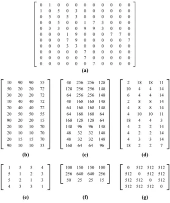
In Figure 7, (a)is the component communica-tion matrixK. The values we use are almost the same as those in standard AHP scale(the com-munication can be: 0 – none, 1 – low, 3 – occa-sional, 5 – moderate, 7 – frequent, 9 – intensive). One can get the values from the number of calls and an average data packet size or measuring data load on the channels between components. Since _T, the resource consumption matrix, is three-dimensional₍components, computational units, resources), we used three tables to dis-play three different resources (i.e. the 3rd di-mension₎;₍b₎average execution time₍ millisec-onds₎,₍c₎memory₍megabytes₎and₍d₎average energy consumption ₍milliamperes per hour₎. Matrix ₍e₎ is the platform communication ma-trix C, (f) is the resource availability matrix

R, and (g) is the bandwidth between compo-nents, matrixB. Since all computational units communicate through common CAN-bus, the bandwidth for communication between them is the same.

Figure 7. The input matrices.

There are also two additional architectural de-cisions to consider:

• Vision component(7-V)should be allocated on GPU.

• Manual drive(4-MD), mission management (5-MM₎and movement control₍6-MC₎ com-ponents should be on FPGAII.

Figure 8. Pairwise comparison(average execution time, memory, energy, communication).

rows and columns of this matrix are: 1)average execution time importance, 2₎ memory impor-tance, 3) energy consumption importance, 4) communication channel load. The importance of resources for our case study is the following (respectively₎: 1₎energy consumption, 2₎ av-erage execution time, 3)memory load, 4) com-munication load(also visible fromF).

Calculated trade-off vector is:

F _{= (}0_.1557_,0_.0856_,0_.7095_,0_.0491₎

with the eigenvalue3 _

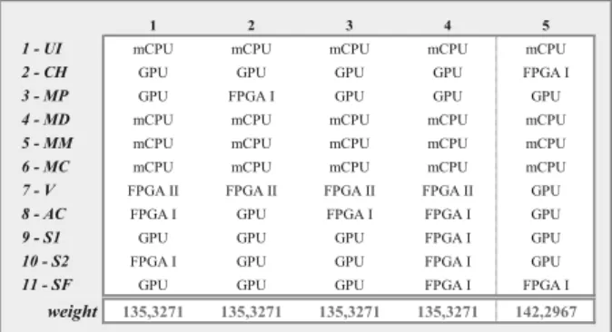
max = 4.2457. Consis-tency ratio is 8_.18%_<10%, hence acceptable. Figure 9 shows the results from five consecu-tive GA executions for data defined in Figure 7. There are small deviations in different solutions. The ones with lowest cost function results 1-4, the fifth result however omits the6-MC_→ FP-GAIIconstraint to demonstrate how this change reflects on the result.

1 2 3 4 5

1 - UI mCPU mCPU mCPU mCPU mCPU

2 - CH GPU GPU GPU GPU FPGA I

3 - MP GPU FPGA I GPU GPU GPU

4 - MD mCPU mCPU mCPU mCPU mCPU

5 - MM mCPU mCPU mCPU mCPU mCPU

6 - MC mCPU mCPU mCPU mCPU mCPU

7 - V FPGA II FPGA II FPGA II FPGA II GPU

8 - AC FPGA I GPU FPGA I FPGA I GPU

9 - S1 GPU GPU GPU FPGA I GPU

10 - S2 FPGA I GPU GPU FPGA I GPU

11 - SF GPU GPU GPU FPGA I FPGA I

weight 135,3271 135,3271 135,3271 135,3271 142,2967

Figure 9. The results of multiple execution of GA

(score: less is better).

Since the solutions 1-4 are valid, software archi-tect can choose, according to some own prefer-ence, one of the solutions. However, he/she is certain that all of them minimize energy con-sumption with regard to given resources. Also notice that user-defined constraints for components 7-V, 4-MD, 5-MM, and 6-MC are taken into account on all the solutions. So com-ponent 7-V is allocated on GPU as requested, while components 4-MD, 5-MM, 6-MC are al-located on multicore CPU.

5. Related Work

There are a lot of component-oriented frame-works for modeling the software architecture listed in[4], that enable reasoning about extra-functional properties (e.g. Palladio component model and performance _[5_], or ProCom com-ponent model and worse-case execution time [6]where software components are allocated on virtual nodes, and later those virtual nodes to physical nodes[7], or in some cases managing deployment, but without optimization _[8_]). A trade-off analysis of utilization of different re-sources in real-time system is discussed in[9]. However, not a lot of work addresses component-oriented frameworks targeted for heterogeneous platform, and specifically allocating software components to heterogeneous computational units. Several works relate to tasks alloca-tion to different processing units with some re-source constraints and to searching for an opti-mal load balancing across the system_[10_],_[11_] or a good average-case performance [12], but they do not address heterogeneous platforms. The second group relates to frameworks where software component allocation is part of the deployment process. Problems related to het-erogeneous platforms and challenges in com-ponents synchronization between the platforms are described in [13]. In [14], a dynamic real-location is enabled in combination with perfor-mance monitoring.

Our method enables efficient placement of soft-ware components on computational units of a heterogeneous platform. It considers multi-ple criteria which are both system-defined and architect-defined. The result is a semi-optimal component allocation for a particular system.

6. Discussion and Future Work

AHP consistency index verification, c) includ-ing the bandwidth constraint for the commu-nication and d) enabled architect defined con-straints.

The solution provides a semi-optimal allocation model which uses a Genetic Algorithm ₍any other optimization technique can be applied) and Analytical Hierarchical Process. The im-proved model presented in this paper provides a strong theoretical basis, however it still needs further refinement due to some initial assump-tions, e.g. deriving input parameters, which is our goal for the future work on this topic, and measuring actual data used for the model. The resource consumption matrixT can be ac-quired by measurements, calculation or empir-ically. For instance, the execution time can be measured as the time which passes from the mo-ment when the input signal arrives to the com-ponent until the output signal exits the compo-nent (i.e. for non-preemptive scheduling) and the task is finished with execution ₍preemptive scheduling).

Communication intensity _K needs further dis-cussion and research. Its intent is to envelop frequency of communication between compo-nents so one can quantify the usage of channels between them. One way to look at it is the number of function calls, channel data type i.e. signal data or streaming data, or the approach which we used in this paper: approximation with AHP scale.

One must also consider non-functional con-straints, e.g. development effort. As shown in Figure 9, first four allocations provide the same result, however different allocations. In real world some components require great de-velopment efforts to be implemented on certain platforms. Partially, this issue is addressed with enabling user preference to the solution. To further address this issue, we can define a new “property” which identifies development cost of each component for particular platform and also express sequential and parallel processing needs.

Further, we also plan to provide a graphical tool with appropriate EMF model which would al-low automatic component allocation in early ar-chitecture design phase. Since this is an ongo-ing research we will also work to improve the

demonstrator (case study) and verify how op-erating system and other platform specific de-pendencies influence the architecture of com-ponents and refine the model accordingly.

7. Acknowledgment

This paper was supported by the Swedish Foun-dation for Strategic Research (SSF) via the project RALF3 [2] and Croatian Ministry of Science, Education and Sport via the project Information Infrastructure and Interoperability.

References

[1] P. LIGGESMEYER, M. TRAPP, Trends in Embed-ded Software Engineering.IEEE Software, 26(3) (2009).

[2] Ralf3 Project Web,http://www.mrtc.mdh.se/ projects/ralf3/,[Accessed: Jan 2013]. [3] AUVSI Fundation Web,

http://www.auvsifoundation.org/

foundation/competitions/robosub/,[

Acces-sed: Jan 2013].

[4] I. CRNKOVIC, S. SENTILLES, A. VULGARAKIS, M.

R. V. CHAUDRON, A Classification Framework for

Software Component Models. IEEE Transactions on Software Engineering,37(5) (2011), 593–615.

[5] S. BECKER, H. KOZIOLEK, R. REUSSNER,

Model-based performance prediction with the Palladio component model.The 6th _{international workshop}

on Software and performance,(2007).

[6] Autosar,http://www.autosar.org/,[Accessed:

Jan 2013].

[7] J. CARLSON, J. FELJAN, J. M ¨AKI-TURJA, M. SJODIN¨ ,

Deployment Modelling and Synthesis in a Compo-nent Model for Distributed Embedded Systems.36th

EUROMICRO Conference on Software Engineering and Advanced Applications (SEAA),(2010), 74–82.

[8] S. SENTILLES, A. VULGARAKIS, T. BURESˇ, J. CARL

-SON, I. CRNKOVIC, A component model for control-intensive distributed embedded systems. 11th

In-ternational Symposium on Component-Based Soft-ware Engineering,(2008), 310–317.

[9] J. FREDRIKSSON, K. SANDSTROM¨ , M. AKERHOLM, Optimizing Resource Usage in Component-Based Real-Time Systems.8th_{International Symposium on}

Component-Based Software Engineering, (2005), 49–65.

[11] S. WANG, J. R. MERRICK, K. G. SHIN, Component

allocation with multiple resource constraints for large embedded real-time software design. 10th

IEEE Real-Time and Embedded Technology and Applications Symposium,(2004), 219–226.

[12] J. FELJAN, J. CARLSON, T. SECELEANU, Towards a

model-based approach for allocating tasks to multi-core processors.38th _{EUROMICRO Conference on}

Software Engineering and Advanced Applications,

(2012), 117–124.

[13] B. Senouci, Multi-CPU/FPGA Platform Based Het-erogeneous Multiprocessor Prototyping: New Chal-lenges for Embedded Software Designers.The 19th

IEEE/IFIP International Symposium on Rapid Sys-tem Prototyping,(2008), 41–47.

[14] S. MALEK, N. MEDVIDOVIC, M. MIKIC-RAKIC, An

Extensible Framework for Improving a Distributed Software System’s Deployment Architecture.IEEE Transactions on Software Engineering, 38(1) (2012), 73–100.

[15] T. L. SAATY, What is the Analytic Hierarchy

Pro-cess? inMathematical Models for Decision Sup-port. Springer, Berlin Heidelberg, 1988, 109–121.

[16] T. L. SAATY,Fundamentals of Decision Making and

Prority Theory with the Analytic Hierarchy Process. Rws Publications, 1994.http://books.google. se/books?id=nmtaAAAAYAAJ

[17] I.SˇVOGOR, I. CRNKOVIC´, N. VRCEKˇ , Multi-Criteria

Software Component Allocation on a Heteroge-neous Platform. In Proc. of 35th _{International}

Conference on Information Technology Interfaces,

(2013)SRCE – University of Zagreb, pp. 341–346.

[18] J. FELJAN, J. CARLSON, The Impact of Intra-core

and Inter-core Task Communication on Architec-tural Analysis of Multicore Embedded Systems.The Eighth International Conference on Software Engi-neering Advances,(October 2013)IARIA, pp. 402–

407.http://www.es.mdh.se/publications/

3021-Received:November, 2013

Revised:January, 2014

Accepted:Junuary, 2014

Contact addresses:

IvanSvogorˇ Department of Information Systems Development Faculty of Organization and Informatics University of Zagreb Croatia e-mail:[email protected] Ivica Crnkovic Software Engineering Division School of Innovation, Design and Engineering M¨alardalen University Sweden email:[email protected] Neven Vrcekˇ

Department of Information Systems Development Faculty of Organization and Informatics University of Zagreb Croatia email:[email protected]

IVANSˇVOGORis a PhD student of information science at the University of Zagreb, Faculty of Organization and Informatics, and a visiting PhD student at M¨alardalen University, Sweden. His research interests in-clude optimization of software component allocation, component based

(software)engineering, heterogeneous embedded systems and robotics software.

IVICACRNKOVICis a professor of industrial software engineering at

M¨alardalen University where he is the scientific leader of the industrial software engineering research group. His research interests include component-based software engineering, software architecture, software configuration management, software development environments and tools, as well as software engineering in general. He is the author of more than 150 refereed publications on software engineering topics and a co-author and co-editor of two books.