On a Computational Method for Non-integer Order Partial Differential Equations in Two Dimensions

Vol. 12, No. 1, 2019, 39-57

ISSN 1307-5543 – www.ejpam.com Published by New York Business Global

On a computational method for non-integer order

partial differential equations in two dimensions

Muhammad Ikhlaq Chohan1_{, Kamal Shah}2,∗

1 _{Department of Business Administration and Accounting Al Buraimi University College,}

Al-Buraimi Sultanate of Oman

2_{Department of Mathematics, University of Malakand, Chakadara Dir(L), Khyber Pakhtunkhwa,}

Pakistan

Abstract. This manuscript is concerning to investigate numerical solutions for different classes including parabolic, elliptic and hyperbolic partial differential equations of arbitrary order (PDEs). The proposed technique depends on some operational matrices of fractional order differentiation and integration. To compute the mentioned operational matrices, we apply shifted Jacobi poly-nomials in two dimension. Thank to these matrices, we convert the PDE under consideration to an algebraic equation which is can be easily solved for unknown coefficient matrix required for the numerical solution. The proposed method is very efficient and need no discretization of the data for the proposed PDE. The approximate solution obtain via this method is highly accurate and the computation is easy. The proposed method is supported by solving various examples from well known articles.

2010 Mathematics Subject Classifications: 35R11, 65M06, 65N30

Key Words and Phrases: Jacobi polynomials, Different classes of partial differential equations, Operational matrix, Algebraic equation, Numerical solution.

1. Introduction

Many phenomenons and problems in biology, physics, chemistry, dynamics, fluid me-chanics, optical technology,etc and in engineering disciplines are modeled by partial dif-ferential equations. The mentioned equations arise in numbers of scientific models like propagation of water waves, long waves and chemical reaction diffusion equations, for de-tail see [7, 29, 36, 40, 41, 41].

Recently, considerable attention has been given to study partial differential equations with non-integer order rather than classical order. Because in many situations, fractional order partial differential equations (FPDEs) modeled real worlds phenomenons more accurately

∗

Corresponding author.

DOI: https://doi.org/10.29020/nybg.ejpam.v12i1.3377

Email addresses: [email protected](M.I.Chohan),[email protected](K. Shah)

as compared to classical order partial differential equations. It has been proved that many interesting process of electromagnetic, acoustics, viscoelasticity, electrochemistry and ma-terial sciences are well described by using fractional order partial differential equations, see [6, 14, 17, 35]. The present work is related to study the following linear FPDE given as



        

        

A∂

α_{w(x, y)}

∂xα +B

∂αw(x, y) ∂xα2y

α 2

+C∂

α_{w(x, y)}

∂yα +D

∂βw(x, y) ∂xβ

+E∂

β_{w(x, y)}

∂yβ +F w(x, y) =g(x, y), α∈(1,2], β ∈(0,1],

corresponding to the initial conditions w(x, y)|x=0 =φ(y), wx(x, y)|x=0 =ψ(y).

(1)

Where A, B, C, D, E, F are real constants and w(x, y) is the solution of the system to be computed and also w(x, y), g(x, y),∈ C([0, δ]×[0, δ]). Under the classical order α = 2, β = 1, the class (1) of FPDEs represents different classes of integer order PDE such as parabolic, ecliptic and hyperbolic partial differential equations. The concerned PDE is parabolic corresponding to integer order if B2_{−4AC = 0, ecliptic if B}2_{−4AC < 0}

and hyperbolic, if B2 −4AC > 0, where each category describes different phenomena in various disciplines of science and engineering. The aforesaid classes of partial differential equations have many applications in various field of science and technology. As Laplace and Poisson equations are ecliptic partial differential equations which have many applica-tions in electromagnetic theory, and other branches of physics, mechanics, etc. Similarly, Heat equation is parabolic and wave equation is hyperbolic partial differential equations. For the importance and uses of these equations, we refe[1, 15, 30, 38]. The area which has greatly attracted the attention of researches is devoted to the existence theory and numerical solution of fractional order partial differential equations. Since the differential equations involved fractional order are not easy to solve for theirs exact solutions in many situations, therefore a strong motivation has been found to find the approximate solutions. In general there does not exist a method which produce exact solutions of FPDEs. In many situations for linear partial differential equations it is quite difficult task to find exact solu-tions. Therefore, numerous techniques were developed to find approximate solutions to the aforementioned equations. In [8, 18], authors applied Homotopy analysis method(HAM) and He’s variation iteration method(VIM) to calculate approximate solutions of nonlinear FPDEs. In same line, authors, used Adomain decomposition method(ADM)[16], homo-topy perturbation method(HPM)[21], Fourier transform method(FTM)[49], Laplace and Natural transform methods[42, 43] to solve fractional order partial differential equation. Also, some authors used fractional differential transform (FDTM)[2, 3, 37], to find numeri-cal solutions of FPDEs. But all these method have their own advantages and disadvantages in application point of view, as homotopy methods depend on small parameters which re-stricted these methods. Similarly the methods that are involving integral transform are also limited in applications.

Recently, numerical schemes based on operational matrices have attracted the attention of many researches. The mentioned techniques provide highly accurate numerical solu-tions to both linear and nonlinear ordinary as well as partial differential equasolu-tions of classical and fractional order. In the concerned schemes some operational matrices of fractional order integration and differentiation are constructed which play central rules in approximation of solutions. In [32, 50], authors used Haar wavelets and Legendre wavelets to solve linear FPDEs. With the same line some operational matrices based on Chebyshev wavelets were also used to find numerical solutions to FPDEs, see [28]. In [4, 5, 9, 26, 33, 48, 51], authors constructed operational matrices based on Lagendre, Bern-stein and Jacobi, Chebyshev polynomials for numerical solutions of fractional differential equations. The concerned method used Tau-collocation method to form the mentioned matrices. As in these methods discretization of date is required which need extra mem-ory but provided best approximate solutions to (FPDEs). To overcome this difficulty, in[22, 23] authors constructed the operational matrices from the afore mentioned poly-nomial directly without discretizing the polypoly-nomials and obtained excellent solutions to (FPDEs). The spectral methods based on operational matrices are the best tools to find approximate solutions for both ordinary and partial fractional differential equations, for detail see[10, 12, 20, 25, 27, 45, 46].

Motivated by the aforesaid work, in this paper we have considered a general multi-terms fractional order partial differential equations which represents different classes of partial differential equations by assigning various values to the constants involved in (1) to satis-fied the specific conditions. The operational matrices involved in this paper are based on shifted Jacobi polynomials. With the the help of these matrices of fractional order inte-gration and differentiation, the considered equation is converted to an algebraic equation which is easily soluble for unknown coefficient matrix needed in the approximate solution. All the computations are done by using Matlab. For the demonstration, we solve different examples of physical interest and also the comparison of our method with other method is provided.

2. Preliminaries

Some auxiliary results and notions needed throughout in this paper are provided as [14]:

Definition 2.1. The Riemann-Liouville integral of arbitrary order α ∈ < of a function

w(x) is defined by

Iαw(x) = 1 Γ(α)

Z x

0

(x−τ)α−1w(τ)dτ,

such that the integral on right hand side converges pointwise on [0,∞). Also the aforesaid

integral satisfies the following relations

(1) Iα_Iβ_{w(x) =I}β_Iα_w(x);

(3) Iα_xγ ₌ Γ(γ+1) Γ(α+γ+1)x

α+γ_.

Definition 2.2. Let w(x)∈C2[0,∞), the arbitrary orderα∈(0,∞) derivative is recalled as

Dαw(x) =

Z x

0

(x−τ)α+1−n

Γ(n−α) w

(n)_{(x)dτ, α∈(n−1, n]; n= [α] + 1,}

where the integral on the right is converges on [0,∞). Further, the operator D satisfies

the following properties in particular for any constant c,Dα_{c= 0 and}

Dα_xi ₌ 





0, i∈N, i <[α], Γ(1 +i)

Γ(1 +i−α)x

i−α_.

The following relations are necessary throughout this paper. Theorem 2.3. For any function w(x), the following results hold.

(a) Dα_Iα_{w(x) =w(x);}

(b) Iα_Dα_{w(x) =w(x)−}Pn−1

i=0 w(i) x

i

Γ(i+1);

(c) Dα_{(λu(x) +µv(x)) =λD}α_{u(x) +µD}α_v(x).

2.1. The shifted Jacobi polynomials

The famous Jacobi polynomials with two parameters sayp, q are defined on [0, δ] as

z(_δ,kp,q)(x) =

i X

k=0

(−1)i−k_{Γ(k+q+ 1)Γ(i+k+p+q+ 1)}

Γ(i+q+ 1)Γ(k+p+q+ 1)Γ(i−k+ 1)Γ(k+ 1)δkx

k_{, i= 0,1,2,3. . . .}

(2) The orthogonality condition is

Z 1

0

z_δ,i(p,q)(x)z_δ,i(p,q)(x)W_δ(p,q)(x)dx=R(_δ,kp,q)∆k,i (3)

where

W_δ(p,q)(x) = (δ−x)pxq (4) is the weight function,

R(_δ,kp,q)∆k,i= z

p+q+1_{Γ(i+p+ 1)Γ(i+q+ 1)}

(2i+p+q+ 1)Γ(i+ 1)Γ(i+p+q+ 1). (5) Thus any any function w(x) which is square integrable in [0, δ] may be approximated interm of shifted Jacobi polynomials as

w(x)≈ n X

l=0

as n → ∞the approximation is converging to the exact function. Inview of (3) (4),(5), we can easily find the constantDl. Writing(6) in matrix form as

w(x)≈HT_NΦˆN(x), (7)

such thatN =n+ 1,KN is the coefficient matrix and ˆΦN(x) is matrix of vectors function.

Extending the notation from uni-dimension to two dimension space in order to define two dimensional shifted Jacobi polynomials of order N over the region [0, δ]×[0, δ] as

z_δ,n(p,q)(x, y) = (z(_δ,kp,q)(x))(z_δ,i(p,q)(y)), n=N k+i+ 1, k, i= 0,1,2, . . . , n. (8)

The orthogonality condition forz(δ,np,q)(x, y) can be computed as

Z δ

0

Z δ

0

(z(_δ,lp,q)(x))(z(_δ,mp,q)(y))(z(_δ,rp,q)(x))(z(_δ,sp,q)(x))W_δ(p,q)(x)W_δ(p,q)(y)dxdy=R(_δ,rp,q)∆l,rR(_δ,sp,q)∆m,s.

(9) An integrable function over the region [0, δ]×[0, δ] is approximated interms of the two-dimensional shifted Jacobi polynomials z(_δ,np,q)(x, y) as

f(x, y)≈ n X

l=0

n X

m=0

Dlm(z(δ,lp,q)(x))(z

(p,q)

δ,m (y)), (10)

whereDlm can be computed as

Dlm=

1

R(_δ,lp,q)R(_δ,mp,q)

Z δ

0

Z δ

0

f(x, y)(z(δ,lp,q)(x))(z

(p,q)

δ,m (y))W

(p,q)

δ (x, y)dxdy, (11)

while

W_δ(p,q)(x, y) =W_δ(p,q)(x)W_δ(p,q)(y). (12) Writing the notation Dn=Dab,then (10) implies

f(x, y)≈ N2 X

n=1

Dnz(_δ,np,q)(x, y) =KNT2Φ_N2(x, y), (13)

whereH_N2 isN2×1 coefficient matrix and Φ_N2(x, y) isN2×1 column matrix of functions

given by

Φ_N2(x, y) = φ₁₁(x, y) · · · φ_1N(x, y) φ₂₁(x, y) · · · φ_2N(x, y) · · · φ_{N N}(x, y) T ,

(14) whereφk+1,i+1(x, y) = (z(_δ,kp,q)(x))(z(_δ,ip,q)(y)), i, k = 0,1,2, . . . , n.

Theorem 2.4. [10, 12, 51] If a continuous functionw(x, y) defined over a region [0, δ]×

of the function converges uniformly to the function. Moreover the error of the approxima-tion for sufficiently smooth funcapproxima-tion w(x, y) over the region [0, δ]×[0, δ]is given by

kw(x, y)−z(N,N)(x, y)k2≤

1

16_(x,y)∈sup[0,1]×[0,1]

4

∂N+1

∂xN+1w(x, y)

+ 4

∂N+1

∂yN+1w(x, y)

+

∂2N+2

∂xN+1_∂yN+1w(x, y)

1 Nn+1

1 Nn+1.

(15)

3. Operational matrices of integrations and differentiations

This section is devoted to construct and recall some operational matrices based on shifted Jacobi polynomials, which are needed throughout in this paper. For the proof of the required operational matrices, see [24].

Theorem 3.1. Consider Φ_N2(x, y) as in given (14), then the α-the order integration of

ΦN2(x, y) corresponding to ‘x0 is provided by

Iα

x(ΦN2(x, y))'S(α,x)

N2_×N2ΦN2(x, y) (16)

with S(_Nα,x2_×)_N2 is the operational matrix given by

S(_Nα,x2_×)_N2 =          

ℵ_1,1,k ℵ_1,2,k · · · ℵ_1,r,k · · · ℵ_1,N2_,k ℵ_2,1,k ℵ_2,2,k · · · ℵ_2,r,k · · · ℵ_2,N2_,k

..

. ... ... ... ... ...

ℵ_v,1,k ℵ_v,2,k · · · ℵ_v,r,k · · · ℵ_v,N2_,k ..

. ... ... ... ... ...

ℵ_N2_,1,k ℵ_N2_,2,k · · · ℵ_N2_,r,k · · · ℵ_N2_,N2_,k           ,

and r=N i+j+ 1, v=N a+b+ 1,ℵq,r,k = Ωi,j,a,b,k for i, j, a, b= 0,1,2, . . . , m,

Ωi,j,a,b,k = a X

k=0

∆a,k,αGi,j,b

Gijb=δj,b i X

l=0

(−1)i−l(2i+p+q+ 1)Γ(i+ 1)Γ(i+l+p+q+ 1)Γ(k+α+l+p+ 1)Γ(p+ 1)δα Γ(i+p+ 1)Γ(l+q+ 1)Γ(i−l+)Γ(l+ 1)Γ(k+α+l+p+q+ 2) .

Where

∆a,k,α=

(−1)a−kΓ(a+q+ 1)Γ(a+k+p+q+ 1)Γ(1 +k)

Theorem 3.2. The fractional order differentiation of Φ_N2(x, y) as defined in (14) corre-sponding to‘y0 as

Dα_y(Φ_N2(x, y))'H(α,y)

N2_×N2ΦN2(x, y) (18)

where H(_Nα,y2_×)_N2 is the operational matrix given as

H(_Nα,y2_×)_N2 =          

ℵ_1,1,k ℵ_1,2,k · · · ℵ_1,r,k · · · ℵ_1,N2_,k ℵ_2,1,k ℵ_2,2,k · · · ℵ_2,r,k · · · ℵ_2,N2_,k

..

. ... ... ... ... ...

ℵ_v,1,k ℵ_v,2,k · · · ℵ_v,r,k · · · ℵ_v,N2_,k ..

. ... ... ... ... ...

ℵ_N2_,1,k ℵ_N2_,2,k · · · ℵ_N2_,r,k · · · ℵ_N2_,N2_,k           , (19)

and v=N i+j+ 1, r=N a+b+ 1,ℵv,r,k= Ωi,j,a,b,k for i, j, a, b= 0,1,2, . . . , n,

Ωi,j,a,b,k = a X

k=0

Λa,k,σ∆i,j,b, (20)

Gijb=δj,b i X

l=0

(−1)i−l(2i+p+q+ 1)Γ(i+ 1)Γ(i+l+p+q+ 1)Γ(k−σ+l+q+ 1)Γ(p+ 1)δα Γ(i+p+ 1)Γ(l+q+ 1)Γ(i−l+ 1)Γ(l+ 1)Γ(k−α+l+p+q+ 2)

(21)

and

∆a,k,α=

(−1)a−kΓ(a+q+ 1)Γ(a+k+p+q+ 1)Γ(1 +k)

Γ(k+q+ 1)Γ(a+p+q+ 1)(a−k)!k!Γ(1 +k−α)δk. (22) In the same line, the fractional order differentiation of Φ_N2(x, y) corresponding to ‘x0 as provided as

Dα_x(ΦN2(x, y))'H(α,x)

N2_×N2ΦN2(x, y), (23)

where H(_Nα,x2_×)_N2 is the operational matrix defined as

H(_Nα,x2_×)_N2 =          

ℵ1,1,k ℵ1,2,k · · · ℵ1,r,k · · · ℵ1,N2_,k ℵ_2,1,k ℵ_2,2,k · · · ℵ_2,r,k · · · ℵ_2,N2_,k

..

. ... ... ... ... ...

ℵ_v,1,k ℵ_v,2,k · · · ℵ_v,r,k · · · ℵ_v,N2_,k ..

. ... ... ... ... ...

ℵ_N2_,1,k ℵ_N2_,2,k · · · ℵ_N2_,r,k · · · ℵ_N2_,N2_,k           . (24)

Theorem 3.3. The fractional order derivative of Φ_N2(x, y) is constructed in (14) corre-sponding to0x0 and 0y0 as

∂α

∂x(α/2)_∂y(α/2)(ΦN2(x, y))'H (α,x,y)

where H(_Nα,x,y2_×N)2 is the operational matrix of given as

H(_Nα,x,y2_×N)2 = 

        

ℵ_1,1,k ℵ_1,2,k · · · ℵ_1,r,k · · · ℵ_1,N2_,k ℵ_2,1,k ℵ_2,2,k · · · ℵ_2,r,k · · · ℵ_2,N2_,k

..

. ... ... ... ... ...

ℵ_v,1,k ℵ_v,2,k · · · ℵ_v,r,k · · · ℵ_v,N2_,k ..

. ... ... ... ... ...

ℵ_N2_,1,k ℵ_N2_,2,k · · · ℵ_N2_,r,k · · · ℵ_N2_,N2_,k 

        

, (26)

and r=N i+j+ 1, v=N a+b+ 1,ℵv,r,k= Ωi,j,a,b,k for i, j, a, b= 0,1,2, . . . , n,

Ωi,j,a,b,k = a X

k=0

∆a,k,αΘi,j,b (27)

Θijb=δj,b i X

l=0

(−1)i−l(2i+p+q+ 1)Γ(i+ 1)Γ(i+l+p+q+ 1)Γ(k−α+l+q+ 1)Γ(p+ 1)δα Γ(i+p+ 1)Γ(l+q+ 1)Γ(i−l+ 1)Γ(l+ 1)Γ(k−α+l+p+q+ 2)

(28)

and

∆a,k,α=

(−1)a−kΓ(a+q+ 1)Γ(a+k+p+q+ 1)Γ(1 +k)

Γ(k+q+ 1)Γ(a+p+q+ 1)Γ(a−k+ 1)Γ(k+ 1)Γ(1 +k−α)δk. (29)

Proof. The operational matrix H(_Nα,x,y2_×N)2 can be easily obtain by using the product of

two operational matrices,H(_Nα,y2_×)_N2 and H

(α,x)

N2_×N2 given in Theorem 3.2.

4. Numerical procedure based on the operational matrices for FPDE (1)

With the help of operational matrices constructed in section 3, the considered class of FPDEs (1) is converted to simple algebraic equations which is easily soluble. Assume that the following hold

∂αw(x, y)

∂xα =KN2ΦN2(x, y). (30)

Then inview of Definition 2.1, we have

w(x, y)−c1−c2y=KN2Sα,x

N2_×N2ΦN2(x, y) (31)

which on using initial conditions of (1) yields that w(x, y) =K_N2Sα,x

N2_×N2ΦN2(x, y) +φ(y) +yψ(y)

=KN2Sα,x

N2_×N2ΦN2(x, y) +L_N2Φ_N2(x, y), whereφ(y) +yψ(y) =L_N2Φ_N2(x, y)

= [KN2S(α,x)

N2_×N2+LN2]Φ_N2(x, y).

Now inview of the relation obtained in (32), we have

∂αw(x, y)

∂yα = [KN2S

(α,x)

N2_×N2 +LN2]H(α,y)

N2_×N2ΦN2(x, y),

∂β_{w(x, y)}

∂xβ = [KN2S

(α,x)

N2_×N2+LN2]H(β,x)

N2_×N2ΦN2(x, y),

∂βw(x, y)

∂yβ = [KN2S

(α,x)

N2_×N2+LN2]H(β,y)

N2_×N2ΦN2(x, y),

∂αw(x, y) ∂xα2∂y

α 2

= [KN2S(α,x)

N2_×N2 +LN2]H(α,x,y)

N2_×N2ΦN2(x, y),

g(x, y) =MN2Φ_N2(x, y).

(33)

Therefore, with the help of (30), (31),(32) and (33), our considered class of FPDEs (1) becomes

AKN2Φ_N2(x, y) +B[K_N2S(α,x)

N2_×N2+LN2]H(α,x,y)

N2_×N2ΦN2(x, y)

+C[KN2S(α,x)

N2_×N2+LN2]H(α,y)

N2_×N2ΦN2(x, y) +D[K_N2S(α,x)

N2_×N2 +LN2]H(β,x)

N2_×N2ΦN2(x, y)

+E[KN2S(α,x)

N2_×N2 +LN2]H(β,y)

N2_×N2ΦN2(x, y) +F[K_N2S(α,x)

N2_×N2 +LN2]Φ_N2(x, y) =M_N2Φ_N2(x, y),

(34)

which on simplification yields

AKN2 +K_N2S(α,x) N2_×N2[BH

(α,x,y)

N2_×N2+CH

(α,y)

N2_×N2 +DH

(β,x)

N2_×N2 +EH

(β,y)

N2_×N2 +FIN2_×N2]

+LN2[BH(α,x,y)

N2_×N2+CH

(α,y)

N2_×N2 +DH

(β,x)

N2_×N2 +EH

(β,y)

N2_×N2 +FIN2_×N2]−M_N2 =O_N2.

(35)

On writing

Q=S(_Nα,x2_×)_N2[BH

(α,x,y)

N2_×N2 +CH

(α,y)

N2_×N2 +DH

(β,x)

N2_×N2 +EH

(β,y)

N2_×N2 +FIN2_×N2],

P=LN2Q−M_N2,

we, have from (35)

AK_N2 +K_N2Q+P=O_N2 (36)

It is obvious that (36) is an algebraic equation of matrices. Solving the (36), for K_N2,

plugging its value in (32), we can get the numerical solution of the problem under consid-eration.

5. Numerical Examples

α L∞ at N = 6 L∞ at N = 8 L∞ at N = 10 L∞ at N = 12 1.5 5.707(−5) 5.3325(−6) 1.6826(−7) 1.6009(−8) 1.6 5.956(−5) 4.0196(−6) 7.0638(−8) 7.5009(−9) 1.7 7.236(−6) 7.1703(−8) 8.9126(−9) 9.9998(−12) 1.8 2.0873(−7) 6.0386(−8) 5.9451(−10) 2.7945(−12) 1.9 9.0002(−8) 1.0158(−9) 3.0781(−11) 1.0520(−14) 2.0 2.5000(−11) 1.0019(−13) 1.0933(−15) 2.0251(−16)

Table 1: Absolute error inw(x, y) of Example 1 for (p, q) = (0,0) and at various values of N

and α.

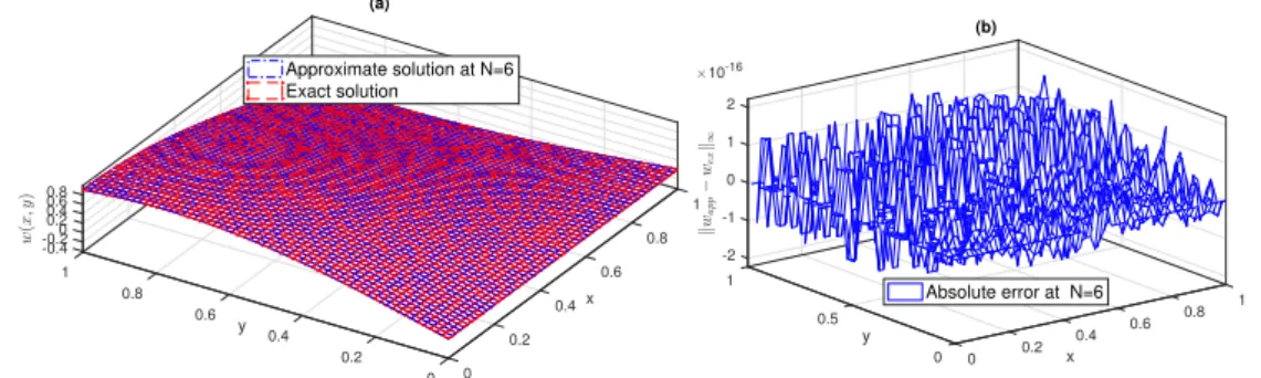
Example 1. Consider the Helmholtz equation [34]

∂α_{w(x, y)}

∂xα +

∂α_{w(x, y)}

∂yα + 8w(x, y) = 0, 1< α≤2,

w(0, y) = sin(2y), wx(0, y) = 0.

(37)

At α= 2 the exact solution of (37) isw(x, y) = cos(2x) sin(2y). Here A = 1, B= 0, C =

1, D = E = 0, F = 8, clearly B2 _{−4AC < 0, the given FPDE is ecliptic. We plot the}

approximate solution corresponding to the exact solution atα= 2. We see from the Figure

1, that the proposed scheme provides close agreement to that of exact solution at very small

scale level. Further, we compared the absolute errorL∞=kw−wNk∞at various fractional

order corresponding to different scale level N in the following Table 1.

x y 1 0.8 -0.4 0.6 1 0.8 0.4 0.6 0.4 0.2 -0.2 0.2 0 0 0 0.2 (a) w ( x , y ) 0.4 0.6 0.8

Approximate solution at N=6 Exact solution y x -2 1 -1 1 0 k w a p p − w e x k∞ ×10-16

0.8 1 (b) 0.5 0.6 2 0.4 0.2 0 0

Absolute error at N=6

Figure 1. (a) Comparison between exact and approximate solutions at

N = 6, p=q = 0, α= 2 for Example 1. (b) Absolute error at N = 6, p=q= 0, α= 2 for

Example 1.

From the Table 1, we see that as the fractional order approaches to its integer values the absolute error decreasing and vice versa and on the other hand enlarging the scale level, the accuracy also increases even for fractional order.

Example 2. Taking FPDE consider in [19]

∂αw(x, y) ∂xα +

∂αw(x, y) ∂xα2∂y

α 2

+ ∂

α_{w(x, y)}

∂yα =g(x, y), 1< α≤2,

w(0, y) = 2y, wx(0, y) =y2.

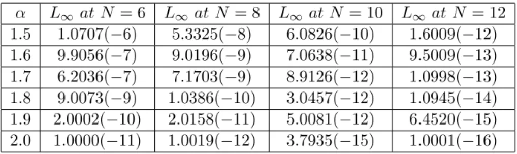
α L∞ at N = 6 L∞ at N = 8 L∞ at N = 10 L∞ at N = 12 1.5 1.0707(−6) 5.3325(−8) 6.0826(−10) 1.6009(−12) 1.6 9.9056(−7) 9.0196(−9) 7.0638(−11) 9.5009(−13) 1.7 6.2036(−7) 7.1703(−9) 8.9126(−12) 1.0998(−13) 1.8 9.0073(−9) 1.0386(−10) 3.0457(−12) 1.0945(−14) 1.9 2.0002(−10) 2.0158(−11) 5.0081(−12) 6.4520(−15) 2.0 1.0000(−11) 1.0019(−12) 3.7935(−15) 1.0001(−16)

Table 2: Absolute error inw(x, y) of Example 2 for (p, q) = (0,0) and at various values of N

and α.

At α= 2 the exact solution of (39) isw(x, y) = 2y+xy2. HereA= 1, B= 1, C = 1, D= E =F = 0, clearly B2−4AC = 0, the given FPDE is parabolic. Also g(x, y) = 2(x+y).

We plot the approximate solution corresponding to the exact solution at α = 2. We see

from the Figure 2, that the approximate solution obtained via adapting procedure gives

close agreement to that of exact solution at very small scale level. We also compute

the absolute error L∞ = kw −wNk∞ for different fractional order using various

val-ues of N in the given Table 2. We observe from the Table 2 that as α approaches to

its integer value, the absolute error decreasing. Similarly, on the other hand

increas-ing the scale level, the accuracy also increases for usincreas-ing different fractional order α.

y x 0 1 0.2 0.4 1 ×10-8 k w e x − w a p p k∞ 0.6 0.8 (b) 0.8 0.5 _0.6 1 0.4 0.2 0 0

Absolute error at N=5

y x 0 1 0.5 1 0.8 ₁ 1.5 w ( x , y ) 2 0.6 0.8 (a) 2.5 0.6 0.4 0.4 0.2 _0.2 0 0

Approximate solution at N=5 Exact solution

Figure 2. (a) Comparison between exact and approximate solutions at

N = 5, p=q = 0, α= 2 for Example 2. (b) Absolute error at N = 5, p=q= 0, α= 2 for

Example 2.

Example 3. Consider the following fractional partial differential equation

5∂

α_{w(x, y)}

∂xα + 6

∂αw(x, y) ∂xα2∂y

α 2

−4∂

α_{w(x, y)}

∂yα + 7

∂βw(x, y) ∂xβ

+ 8∂

β_{w(x, y)}

∂yβ + 9w(x, y) =g(x, y),

w(0, y) = 0, wx(0, y) = 0.

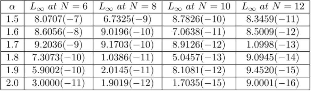
α L∞ at N = 6 L∞ at N = 8 L∞ at N = 10 L∞ at N = 12 1.5 8.0707(−7) 6.7325(−9) 8.7826(−10) 8.3459(−11) 1.6 8.6056(−8) 9.0196(−10) 7.0638(−11) 8.5009(−12) 1.7 9.2036(−9) 9.1703(−10) 8.9126(−12) 1.0998(−13) 1.8 7.3073(−10) 1.0386(−11) 5.0457(−13) 9.0945(−14) 1.9 5.9002(−10) 2.0145(−11) 8.1081(−12) 9.4520(−15) 2.0 3.0000(−11) 1.9019(−12) 1.7035(−15) 9.0001(−16)

Table 3: Absolute error inw(x, y) of Example 3 for (p, q) = (0,0) and at various values of N

and α.

At α= 2, β= 1 the exact solution of (39) is w(x, y) = (xy)4−(xy)3. Here

A= 5, B= 6, C =−4, D= 7, E = 8, F = 9. As B2−4AC >0, the given FPDE is hyperbolic.

In the Figure ??, we have plotted the approximate solution corresponding to the exact

solution atα= 2. We see that the approximate solution obtained via proposed method

has the close agreement to that of exact solution at sufficiently small scale level. Further,

we compute the absolute error L∞=kw−wNk∞ for different fractional order and using

various values of N in the given Table 3. We observe from the Table 3 that as α

approaches to its integer value, the absolute error decreasing. Similarly, by increasing the scale level, the accuracy also increases for taking different fractional order.

x y

0 1 1

1 2

k

w

a

p

p

−

w

e

x

k∞ ×10-11

0.8

(a)

3

0.5 _0.6

4

0.4 0.2 0 0

Absolute error at N=6

x

w

(

x

,

y

)

y 1

-0.1

1 0.8

0.8 0.6

0.6 0.4

0.4

0.2 0.2

0 0 -0.05

(b)

0

Approximate solution at N=6 Exact solution

Figure 3. (a)Absolute error at N = 6, p=q = 0, α= 2, β= 1 for Example 3. (b)

Comparison between exact and approximate solutions at N = 6, p=q= 0, α= 2, β= 1

for Example 3.

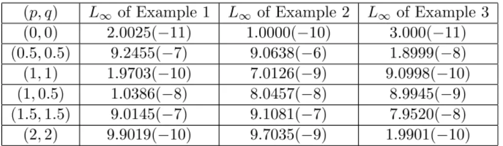
Remark 1. The numerical solutions of FPDEs by using shifted Jacobi polynomials are also depending on the values of the parameters of the considered polynomials. Therefore the absolute error also depends upon on the values of the Jacobi polynomials parameters. We give the following Table 4, for all three examples and the absolute error at scale level

N = 6 and taking fractional orderα= 1.8. We see that as the values of parameters (p, q)

(p, q) L∞ of Example 1 L∞of Example 2 L∞ of Example 3 (0,0) 2.0025(−11) 1.0000(−10) 3.000(−11) (0.5,0.5) 9.2455(−7) 9.0638(−6) 1.8999(−8) (1,1) 1.9703(−10) 7.0126(−9) 9.0998(−10) (1,0.5) 1.0386(−8) 8.0457(−8) 8.9945(−9) (1.5,1.5) 9.0145(−7) 9.1081(−7) 7.9520(−8) (2,2) 9.9019(−10) 9.7035(−9) 1.9901(−10)

Table 4: Absolute error inw(x, y) of Example 3 at various values ofN and α.

6. Comparison of the proposed method with some already existing Haar wavelet method

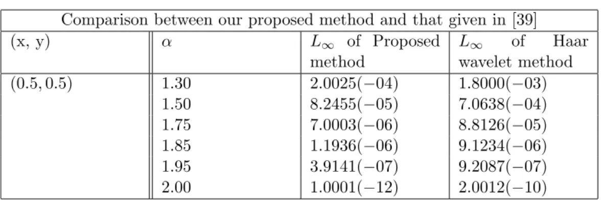
The Shifted Legendre polynomials are the special case of Shifted Jacobi polynomials and they can be obtained by p = q = 0, δ = 1 in the relation (2). We compared our technique with the existing methods available in [39], where the authors constructed the procedure by discretizing the data and using the Haar wavelet method, which need extra memory to obtained the operational matrices of fractional derivative and integration because data need discretization and collocation. While in our prosed method, we have obtained the operational matrices without discretization of data and using any collocation method. In the following examples we provide the comparison of the proposed method with the existing some methods.

Example 4. Consider the given equation as

∂αw(x, y) ∂xα +

∂α−1w(x, y)

∂xα−1 +w(x, y) =

∂2w(x, y) ∂y2

+

Γ(2α+ 1) Γ(α+ 1)

1 + x α+x

−xα

x2αcos(7y), 1< α≤2,

w(0, y) = 0, wx(0, y) = 0, w(0, x) =x2α, w(1, x) = 0.7539022x2α.

(40)

The exact solution of the problem (40) is

Comparison between our proposed method and that given in [39]

(x, y) α L∞ of Proposed

method

L∞ of Haar wavelet method (0.5,0.5) 1.30 2.0025(−04) 1.8000(−03)

1.50 8.2455(−05) 7.0638(−04) 1.75 7.0003(−06) 8.8126(−05) 1.85 1.1936(−06) 9.1234(−06) 1.95 3.9141(−07) 9.2087(−07) 2.00 1.0001(−12) 2.0012(−10)

Table 5: Comparison of the absolute errors for the solution w(x, y) of Example 4 at various

values of αandN = 10.

y

x

1 0.8

1 0.6

0.8

0.4 0.6

-0.5

0.4 0.2

0.2 0 0 0

w

(

x

,

y

)

(a)

0.5 1

Approximate solution at N=6

Exact solution kw

a

p

p

−

w

e

x

k∞

x y

1 -1

1 0

×10-8

0.8

(b)

1

0.5 _0.6

0.4 0.2 0 0

Absolute error at N=6

Figure 3. (a) Comparison between exact and approximate solutions at

N = 6, p=q= 0, α= 1.9, for Example 4. (b) Absolute error at

N = 6, p=q = 0, α= 1.9,for Example 4

Similarly, we can also bring out comparison for other problems of FDEs and FPDEs. From the Table 5, it is clear that the proposed method provides powerful tools to obtain approximate solutions which is closely related with the exact solution of the problem.

Conclusion

memory and waste of time and suffers from computational complexity some times. All these mentioned things are avoided in this method and a direct computational procedure has been adopted. In future this method, we can easily extended to nonlinear FPDEs.

ACKNOWLEDGEMENTS We are very thankful to the reviewers for their useful suggestions/corrections which improved this manuscript very well.

References

[1] I Aksikas, A Fuxman, J F Forbes, J Winkin. LQ control design of a class of hyperbolic PDE systems: Application to fixed-bed reactor. Automatica,45: 1542–1548, 2012. [2] E Abuteen, A Freihat, M Al-Smadi, H Khalil, R A Khan: Approximate series solution

of nonlinear, fractional Klein-Gordon equations using fractional reduced differential transform method.Journal of Mathematics and Statistics,12(1): 23–33, 2016. [3] M Al-Smadi, A Freihat, H Khalil, S Momani, R A Khan. Numerical multistep

ap-proach for solving fractional partial differential equations. International Journal of

Computational Methods, 14: 1-15, 2017.

[4] M Al-Smadi and O A Arqub. Computational algorithm for solving fredholm time-fractional partial integrodifferential equations of dirichlet functions type with error estimates.Applied Mathematics and Computation,342: 280–294, 2019.

[5] O A Arqub and M Al-Smadi. Numerical algorithm for solving time-fractional par-tial integrodifferenpar-tial equations subject to inipar-tial and Dirichlet boundary conditions.

Num. Meth. Partial Differential Equations,34(5): 1577–1597, 2018.

[6] K B Oldham. Fractional differential equations in electrochemistry. Adv. Eng. Soft,

41: 9–12, 2010.

[7] P J Caudrey, I C Eilbeck, J D Gibbon, The sine-Gordon equation as a model classical field theory.Nuovo Cimento,25:497–511, 1975.

[8] M Deghan, Y A Yousefi, A Lotfi. The use of He’s variational iteration method for solving the telegraph and fractional telegraph equations. Comm. Numer. Method.

Engrg., 27: 219–231, 2011.

[9] E H Doha, A H Bhrawy, D Baleanu and S S Ezz-Eldien. The operational matrix formulation of the Jacobi Tau approximation for space fractional diffusion equation.

Adv. Differ. Equns.,231 :1687–1847, 2014.

[11] A Freihat, R Abu-Gdairi, H Khalil, E Abuteen, M Al-Smadi, R A Khan. Fitted reproducing kernel method for solving a class of third-order periodic boundary value problems.American Journal of Applied Sciences,13 (5): 501–510, 2016.

[12] M Gasea, T Sauer. On the history of multivariate polynomial interpolation.J. Comp.

App.Math,122: 23–35, 2000.

[13] T Hayat, F Shahzad, M Ayub. Analytical solution for the steady flow of the third grad fluid in a porous half space.Appl. Math. Model.,31: 243–250, 2007.

[14] R Hilfer. Applications of fractional calculus in physics. World Scientifc Publishing Company, Singapore, 2000.

[15] W Hackbusch.Elliptic Differential Equations: Theory and Numerical Treatment. Vol-ume 18 of Springer Series in Computational Mathematics, Springer, Berlin, 1992. [16] Y Hu, Y Luo and Z Lu. Analytical solution of the linear fractional differential equation

by Adomian decomposition method.J.Comput. Appl. Math., 215: 220 – 229, 2008. [17] H Jafari, S Seifi. Homotopy analysis method for solving linear and nonlinear fractional

diffusion-wave equation. Common. Nonl. Sci. Numer. Simul., 14 (5) : 2006–2012, 2009.

[18] H Jafari and S Seifi. Solving a system of nonlinear fractional partial differential equa-tions using homotopy analysis method. Commun. Nonl. Sci. Num. Simun.,14:1962 – 1969, 2009.

[19] M A Jafari and A Aminataei. Improved homotopy purturbation method.Int. Math.

Forum,32(5): 1567–1579, 2010.

[20] S Kazem, S Abbasbandy, S Kumar. Fractional-order Legendre functions for solving fractional-order differential equations. Applied Mathematical Modelling, 37: 5498– 5510, 2013.

[21] D Kumar, J Singh and S Kumar. Numerical computation of fractional multi-dimensional diffusion equations by using a modified homotopy perturbation method.

J. Association of Arab Universities for Basic and Applied Sciences,17:20–26, 2015.

[22] H Khalil, R A Khan. A new method based on Legendre polynomials for solutions of the fractional twodimensional heat conduction equation.Comput.Math. Appl., 67:1938– 1953, 2014.

[24] H Khalil, R A Khan, M Al-Smadi, A Freihat. Approximation of solution of time fractional order three-dimensional heat conduction problems with Jacobi Polynomials.

Punjab University Journal of Mathematics,47: 35–56, 2015.

[25] H Khalil, R A Khan, M Al-Smadi, A Freihat, N Shawagfeh. New operational matrix for shifted Legendre polynomials and fractional differential equations with variable coefficients.Punjab University Journal of Mathematics, 47: 81–103, 2015.

[26] H Khan, M Alipour, R A Khan, H Tajadodi and A Khan. On Approximate Solu-tion of FracSolu-tional Order Logistic EquaSolu-tions by OperaSolu-tional Matrices of Bernstein Polynomials.J. Math. Computer Science, 14: 222–232, 2015 .

[27] M M Khader, A S Hendy. The approximate and exact solutions of the fractional-order delay differential equations using Legendre seudospectral method the approximate and exact solutions of the fractional-order delay differential equations using Legendre seudospectral method.Int. J. Pure and Appl. Math., 74 (3): 287–297, 2012.

[28] Y Li. Solving a nonlinear fractional differential equation using Chebyshev wavelets.

Nonlinear Sci. Numer. Simul.,15:2284–2292, 2010.

[29] S Linge, J Sundnem, M Hanslien, GT Lines, A Tveito. Numerical solution of the bidomain equations. Philosophical Transactions, Series A: Mathematical, Physical

and Engineering Sciences,367: 1931–1950, 2009.

[30] A A Moghadam, I Aksikas, S Dubljevic, J F Forbes. LQ control of coupled hyper-bolic PDEs and ODEs: Application to a CSTR-PFR system. Proceedings of the 9th International Symposium on Dynamics and Control of Process Systems (DYCOPS 2010), Leuven, Belgium, July 5-7, 2010.

[31] A Mohebbi, M Abbaszadeh and M Dehghan. The use of a meshless technique based on collocation and radial basis functions for solving the fractional nonlinear schrodinger equation arising in quantum mechnics.Eng. Anal. Bound. Elem.,37: 475–485, 2013. [32] M A Mohamed and M S Torky. Solution of Linear System of Partial Differential Equations by Legendre Multiwavelet and chebyshev multiwavelet. Int.J. Sci.Inno.

Math. Research,2(12): 966–976, 2014.

[33] S Momani, O A Arqub, T Hayat, H Al-Sulami. A computational method for solv-ing periodic boundary value problems for integro-differential equations of Fredholm-Volterra type.Applied Mathematics and Computation,240(1): 229–39, 2014.

[34] S T Mohyud-Din and MA Noor. Homotopy purturbation method for solving partial differential equations.Z.Naturforsch,64a: 157–170, 2009.

[36] S Wensheng.Computer Simulation and Modeling of Physical and Biological Processes

using Partial Differential Equations, University of Kentucky Doctoral Dissertations,

2007.

[37] Z Odibat and S Momani. A generalized differential transform method for linear partial differential equations of fractional order,Appl. Math. Lett.,21(2):194–199, 2008. [38] V Parthiban and K Balachandran. Solutions of System of Fractional Partial

Differ-ential Equations.Appl.Applied Mathematics, 8(1): 289 – 304, 2013.

[39] M Rahman. Boundary Value Problems for Fractional Differential Equations: Exis-tence Theory and Numerical Solutions. PhD thesis, Nust University, Pakistan, 2011. [40] J Sundnes,GT Lines, KA Mardal, A Tveito, Multigrid block preconditioning for a coupled system of partial differential equations modeling the electrical activity in the heart.Comput. Method.Biomech. Biomed. Eng.,5(6): 397–409, 2002.

[41] J Sundnes, GT Lines, A Tveito. An operator splitting method for solving the bido-main equations coupled to a volume conductor model for the torso. Mathematical

Biosciences,194(2):233–248, 2005.

[42] J Singh, D Kumar, S Kumar. New treatment of fractional Fornberg-Whitham equa-tion via Laplace transform.Ain Sham Eng. J., 4: 557–562, 2013.

[43] K Shah, H Khalil and RA Khan. Analytical solutions of fractional order diffusion equations by natural transform method. Iran. J. Sci. Technol: Trans Sci A, 2016 : 12 pages, 2016.

[44] R Saadeh, M Al-Smadi, G Gumah, H Khalil, R A Khan. Numerical Investigation for Solving Two-Point Fuzzy Boundary Value Problems by Reproducing Kernel Ap-proach.Applied Mathematics & Information Sciences, 10(6): 1–13, 2016.

[45] K Shah, A Ali and R A Khan. Numerical solutions of Fractional Order System of Bagley-Torvik Equation Using Operational Matrices. Sindh Univ. Res. J., 47(4) : 757–762, 2015.

[46] A Saadatmandi and M Deghan. A new operational matrix for solving fractional-order differential equation.Comp. Math. Appl.,59:1326–1336, 2010.

[47] M Uddin and S Haq. RBFs approximation method for time fractional partial differ-ential equations.Commun. Nonlinear Sci.Numer.Simul, 16 :4208–4214, 2011.

[48] Y Wang and Q Fan. The second kind Chebyshev wavelet method for solving fractional differential equation.Appl. Math. Comput.,218: 85–92, 2012.

[50] M Yi and Y Chen. Haar wavelet operational matrix method for solving fractional partial differential equations.Appl. Math.Comput.,282(17) :229–242, 2012.