Structural Join Algorithm for
Sequential Regular Path Expressions
Oleksandr Logvynovskiy
1and Kevin L¨u
2 1SCISM, South Bank University, London, UK2School of Business and Management, Brunel University, Uxbridge, UK
XML queries employ regular path expressions to find structural patterns within XML documents. The opera-tion of structural join is a crucial part of XML query processing. Existing approaches reduce complex join expressions to several binary structural joins. It implies generation of superfluous intermediate data. In this paper, we propose a new structural join algorithm, called sequence join algorithm, for sequential regular path expressions. It exploits information about position of the elements in the document to skip generation of the redundant intermediate lists. The algorithm performs merge of several input lists of nodes in one pass. Experi-mental results prove the algorithm is better than multiple binary join algorithm for queries of both small and large cardinality.
Keywords: XML document, regular path expression, structural join algorithm.
1. Introduction
Extensible Markup Language (XML) is now used as thede factomeans to handle semistruc-tured data over the Web 1]. Semistructured data arises when a data source does not im-pose a rigid structure and/or data is combined from several heterogeneous sources. The power of XML is in its ability to describe hierarchical structures and extend the dictionary of available data types.
XML documents are described in terms of ele-ments 8]. The elements are enfolded by tags, which represent their type names. Each element is either treated as a container for some other elements or associated with an atomic value (such as text, multimedia content, etc.). Struc-tural relationships among the elements are de-fined by nesting(containment)of the elements or by referencing.
A query over the XML data specifiesstructural patternsamong the elements in the document. The result of such a query is intended to lo-cate all occurrences of these patterns within the XML document or database. Such pat-terns are also known asregular path expressions
(RPEs) and constitute the basis for the state-ments of XML query languages, for instance XQuery11], Lorel5], XML-QL7], XPath9], etc. For example, the XQuery path expression //project/task/resource/namespecifies the retrieval of the names of all resources assigned to the tasks of the project.
The specified structural patterns are often com-plex themselves, but can be decomposed into a set of basic structural relationships between elements. Finding matches of the query against the database can then be considered as match-ing each of the basic structural relationships against the data and following merging of the sub-results. This process is performed by means of a structural join operation 2]. The ope-ration essentially depends on finding ances-tor-descendant and parent-child relationships among nodes of the semistructured database. The effective implementation of the structural join operation over ancestor-descendant( parent-child)pattern is the crucial part of XML query processing.
document within the XML database; Start-Pos, EndPos are the text positions of the first and the last character of the element within the document respectively, andLevelis the nesting depth of the element within the document 6]. The alternative representations of the element position preserve the DocID and Level com-ponents of the tuple, but differ in the way to define the start and end positions within the document. For example, there is another repre-sentation(DocID, PrePos, PostPos, Level), which uses the position numbers assigned to the element by pre-order (PrePos) and post-order(PostPos)traversals of the document tree accordingly. The other approaches are equiva-lent to the latter one and can be transformed by appropriate mapping.
The key idea underlying the implementation of the existing join algorithms is the decom-position of the original query path expression into a set of simple (binary) path expressions. Each binary expression produces an interme-diate join result, which is used on the subse-quent stage. For example, the path expres-sion //project/task/resource/name can be decomposed to project/task and resource/ name. Then the intermediate results are joined together. At each of the stages, the join al-gorithm uses element numbering to check the ancestor-descendant or parent-child relation be-tween the nodes.
The XISS system3]introduces three join algo-rithms: element-attribute (EA-join), element-element (EE-join), and Kleene-closure ( KC-join). The element-attribute algorithm joins two intermediate results from subexpressions, which are a list of elements and a list of at-tributes. The element-element algorithm joins two lists of elements. The principal differ-ence between these algorithms is that the lat-ter one checks ancestor-descendant relation-ship between each pair of the input lists while the former one tests parent-child relationship. The Kleene-closure algorithms iteratively use element-element algorithm to compute closure of the expression. It repeatedly applies EE-join to the result from the previous stage of iteration. Both EA-join and EE-join algorithms have a loop over one input list nested into a loop over another list and, therefore, have time complex-ityO(jE1j jE2j), which is quadratic in the size of the input lists. As KC-join depends upon EE-join, it also has quadratic time complexity.
Structural join algorithms proposed by Al-Kha-lifa et al. 2] exploit the advantage of ele-ment numbering to decrease the time of pro-cessing. The tree-merge join algorithm is an extension of relational equality merge join per-formed on sorted inputs. It was adopted to deal with ancestor-descendant or parent-child tests. The time complexity of the tree-merge join is non-quadraticO(jE1j+jE2j), but may include multiple passes over the same input set of de-scendant nodes. To avoid this problem, the sec-ond of the proposed algorithms, stack-tree join algorithm, utilises stack of nodes and has time complexityO(jE1j+jE2j)=B), where B is the blocking factor.
The main drawback of the considered algo-rithms is their limitation to merge only two in-put lists per join. It means that for a sequential regular path expression there may be generated several intermediate results. For example, pro-cessing the path expression //project/task/ resource/nameresults in two joins (project/ task) and (resource/name). Then, yet an-other join is performed to merge intermediate results. This requires additional time to create and scan intermediate data: two intermediate tables will be created and scanned. This factor becomes even more important when processing big semistructured databases. Our approach al-lows to reduce intermediate processing by si-multaneous merging of several inputs. For the given example, it will require only one join ope-ration instead of three.
Bruno et al. have extended the structural join al-gorithm to avoid multiple binary joins and fur-ther merge of intermediate results 10]. The introduced twig join algorithm uses stacks to store elements of the paths successfully tested against a query. Although this is similar to our approach, we exploit numbering, not only for elimination of unnecessary ancestor-descendant checks within the current element subtree, but for fast skipping of entire subtrees.
The rest of the paper is organised as follows. Section 2 presents background material (data model, query expressions, structural relation-ships and element numbering). In section 3 we develop the structural join algorithm for regular path expressions. Section 4 addresses experi-mental aspect and evaluates the proposed algo-rithm. Section 5 summarises results of the paper and discusses future work.
2. Background and Overview
The XML data can be modelled either as a tree or as a graph. The tree model reflects the logi-cal structure of an XML document. Nodes of the tree correspond to the elements of the docu-ment. Nesting of the elements is reflected by the parent-child relationships among nodes. Some of the tree nodes have as their values references to other elements (usually in form of IDREF attributes). The graph model extends the tree by treating such reference nodes as arcs5]. Al-though the graph model is more powerful than the tree, it challenges more problems, like cycle-references.
As this paper concentrates on handling ancestor-descendant relationship, we use a tree data mo-del. The tree model can be used both to store
and query semistructured data2], 3]. Within the XML database, the order numbers of the tree node, along with its depth level and doc-ument number, are used to find the structural relationships between these nodes. This section describes the tree data model and introduces basic structural relationships used for querying XML documents. Then it explains the node po-sition notion and its usage for finding structural relationships between the nodes.
2.1. Data Model
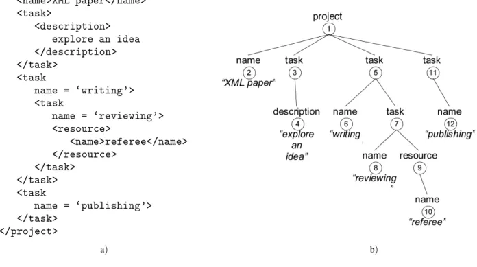
An XML database is a forest of trees corre-sponding to each document within the database. An XML document is a rooted, ordered, la-belled tree. Each element of the document forms anode of the tree labelled with the ele-ment type (tag name) and value. The edges of the tree stand for parent-child(containment) relationship between the elements. All sub-elements nested within the element appear in the tree as the child nodes directly connected with the edges to a parent node. Attributes of the element are represented similarly to nested sub-elements and form additional nodes in the tree, emanating from their associated parent nodes.
<project>
<name>XML paper</name> <task>
<description> explore an idea </description> </task>
<task
name = `writing'> <task
name = `reviewing'> <resource>
<name>referee</name> </resource>
</task> </task> <task
name = `publishing'> </task>
</project>
a) b)
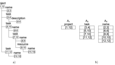
An example of the XML data is shown in Fig-ure 1(a)and its tree representation is shown in Figure 1(b).
The XML data tree has an implicit order of its nodes. The total order of all the nodes in the tree is obtained by a pre-order tree traversal(a depth-first, left-to-right traversal of the nodes). The nodes order of our example tree is shown in Figure 1(b)within the circles of corresponding nodes.
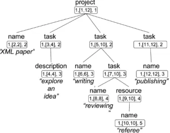
We exploit the order of the nodes in the data tree to compute position of the element in the database. Apositionof the element is a 4-tuple
(DocID, StartInt, EndInt, Level). DocID is the identifier of the XML document within the XML database, StartInt is the tree order number of the node corresponding to the ele-ment, EndPos is the tree order number of the last descendant of the node, and Level is the nesting depth of the node within the tree. For the given example in Figure 2, the positions of the nodes are shown within rectangles. Con-sider, for instance, the node “resource”. Its first position number stands for document identifier and equals to 1. The second and third posi-tion numbers represent the interval of the node
9,10]: order number of the node itself(9)and order number of the last descendant(10), node “name/"referee"”. The last position number shows depth of the node within the tree and equals to 4. The position numbers of all other nodes are computed in the analogous way.
Fig. 2.Positions of the elements.
The position of the node is used to determine structural relationships between any two nodes of the tree.
2.2. Structural Relationships
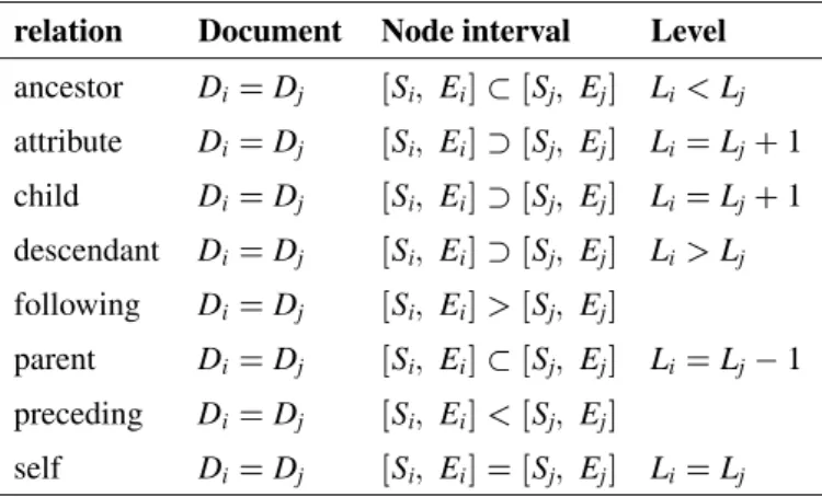
Relationships between a node and the other nodes in the tree are not limited by implicit containment(parent-child)relationship and de-scribed by axes of the node11]. Anaxis is a relation that parts the set of all the tree nodes into subsets with respect to the current node. The most commonly used axes of the node are summarised in Figure 3(a).
axis name description
ancestor ancestors of the node attribute attributes of the node child children of the node descendant descendants of the node following all nodes after the node parent parent of the node preceding all nodes before the node self node itself
a) b)
The ancestor, descendant, following, preceding, and self axes partition document nodes into non-overlapped subsets, as it is shown in Figure 3 (b). The child axis is the subset of the descen-dant axis and the parent axis is the subset of the ancestor axis.
A regular path expression or location path of a target node B from source node A(hereafter referred to as path)is asequenceof nodes in the tree, from the node A to the node B. Relation-ships between intermediate nodes in the path are described by axes. A location path is called
absolute pathif its source node is the root of the tree, otherwise it is calledrelative path.
Regular path expressions are an essential com-ponent of semistructured data query languages
(e.g. XQuery 11]), which utilise variety of structural relationships between the nodes.
2.3. Handling Structural Relationships by Means of Position
Position is an important characteristic of ele-ments within XML docuele-ments and it is intensely used for indexing and querying semistructured data.
Thepositionof the nodeniis denoted as(Di Si, Ei] Li), whereDi is the identifier of the XML document within the XML database; Si is the
tree order number of the nodeni,Ei is the tree
order number of the last descendant of the node
ni, and Li is the nesting depth of the node ni
within the tree. The pair of the node order Si
and order of its last descendantEiconstitutes an
interval of descendant order numbers SiEi]. Hereafter, we will refer to the intervalSiEi]as thenode interval.
Ancestor-descendant relationship. Given a tree nodeniand its position(Di Si Ei] Li)and a tree nodenjand its position(Dj Sj Ej] Lj), the node ni is an ancestor of the node nj (and nodenjis a descendant of the nodeni)iff: a) Di=Dj, i.e. both nodes belong to the same
document;
b) Si Ei] Sj Ej], the node interval of the ancestor includes the interval of the descen-dant, i.e.Si <SjandEi>Ej.
Parent-child relationship. Given a tree node
ni and its position (Di Si Ei]Li) and a tree node nj and its position(Dj Sj Ej] Lj), the nodeniis a parent of the nodenj (and nodenj is a child of the nodeni)iff:
a) Di =Dj, i.e. both nodes belong to the same document;
b) Si Ei] Sj Ej], the node interval of the ancestor includes the interval of the descen-dant, i.e.Si <SjandEi>Ej;
c) Li=Lj;1, the descendant is nested imme-diately within the ancestor node.
For instance, consider the nodes “project” and “resource” in Figure 2. Their document ID numbers coincide and equal to 1. The node interval of “project” includes the interval of the “resource”, 1,12] 9,10], so the “project” is the ancestor of the “resource”. The difference between their levels exceeds 1, so they are not bounded by parent-child relationship.
relation Document Node interval Level ancestor Di=Dj Si Ei] Sj Ej] Li<Lj
attribute Di=Dj Si Ei]Sj Ej] Li=Lj+1
child Di=Dj Si Ei]Sj Ej] Li=Lj+1
descendant Di=Dj Si Ei]Sj Ej] Li>Lj
following Di=Dj Si Ei]>Sj Ej]
parent Di=Dj Si Ei] Sj Ej] Li=Lj;1
preceding Di=Dj Si Ei]<Sj Ej]
self Di=Dj Si Ei]=Sj Ej] Li=Lj
The other structural relationships between any two nodes can be verified by analogy. They are summarised in Table 1.
In Figure 2, the node “description” precedes the node “resource” as they have the same document number and the interval of the “de-scription” occurs before the interval of the “re-source”,4,4]<9,10].
The operational cost to check any of the struc-tural relationship includes document ID, node interval, and level comparison. The costs are equal for any type of relationship, but the an-cestor-descendant and parent-child are the ones mostly used.
3. Algorithm
In this section, we develop new structural join algorithm, in order to efficiently process regular path expression queries. It exploits the concept of node position to merge several input lists in one pass. As it processes several binary struc-tural relationships that form a sequence, we call itsequence joinalgorithm.
At the outset, we consider two ways of result representation(a tree-like form and tuples)and show the algorithm in action on a detailed ex-ample. Then we present algorithm itself and conclude with analytical estimation of its per-formance.
3.1. Representation of the Results
The results of the XML query can be repre-sented either as a tree or as a list of tuples. Con-sider the following query example//project// task//name performed over the data shown in Figure 2. The query retrieves the names of the elements assigned to all tasks within the project (including names of the tasks themselves). The tree and the tuples of the result are shown in Figure 4 a)and b)respectively.
These two forms are equivalent and can be trans-formed from one to another. The tree repre-sentation can be obtained from the tuples by eliminating duplicates of the nodes.
The tree view is more compact and suitable for the data that originally has tree-like structure. Nevertheless, it may fit in applications that need
a) b)
Fig. 4.Forms of query results: tree and tuple.
results in a table-like form. In such a case, tuple representation is more appropriate. Final de-cision on which of the two forms is preferable should be made for each particular case. Hereafter, we use tree representation of the re-sults, adding, if necessary, some comments on the tuple form.
3.2. Example
For the purpose of clarity, we demonstrate the algorithm on an example, before introducing it more formally.
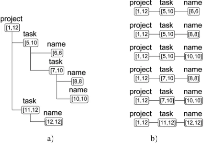
Consider the query expression //project// task//nameapplied to the data in Figure 2. The simplified data tree is presented in Figure 5 a). The document number and level components of the node position are omitted. Thedocument numberis equal for all the nodes of the exam-ple andlevelis not important as no parent-child relationship is tested through the query process-ing. The input lists of the example are shown in Figure 5 b). The list A1 represents the re-sult of select operation and contains all nodes “project” selected from the database. Analo-gously, the listsA2andA3include nodes “task” and “name” respectively.
The steps of the algorithm for the chosen ex-ample are shown in Figure 6. The current node of each list is marked by arrow. For each input list, the algorithm keeps value of a current node
a) b)
Fig. 5.Example of data tree and input lists.
same list. For example, the interval of the node “task 5,10]” in Figure 5 a) is equal to 5,10] and includes six nodes 5 to 10. The range of the same node is equal to 5,10] too, but includes only two “task” nodes 5 and 7. In Figure 6, the range is shown in grey colour. Addition-ally, each of the lists is visually extended with empty cells to show precedence of the nodes in the source tree. For example, the range2,2]of the listA3in Figure 6 a)is preceding the range
3,4]of the listA2and is part of(included into) the range1,12]of the listA1.
The basic idea of the algorithm is to synchrono-usly read input lists to find first match of the ranges. Once the matching ranges are found, the current nodes within ranges are put into the result list. If the ranges in two adjacent lists do not match, then one of the ranges changes, based on the result of their comparison. The propagation of changes goes from the last list
a) b) c)
d) e) f)
back to first. The algorithm stops when no more matches of the ranges can be found.
For the given example, the algorithm starts from the state in Figure 6 a). The ranges are initially assigned to the first nodes of the lists. The comparison of the ranges goes from the list of ancestors to the list of descendants(left-to-right in the figure). The range3,4]of the descendant listA2 satisfies the range1,12]of the ancestor listA1, but the range2,2]of the descendant list A3 is not included into the range 3,4] of the ancestor listA2. As the descendant range2,2] precedes the ancestor range3,4], the algorithm reads a new node from the listA3and changes range to6,6], as it is shown in Figure 6 b). Now the descendant range 6,6] follows the ancestor range 3,4]. Therefore, the latter is changed to5,10](Figure 6 c). At this point, all descendant ranges satisfy the ancestor ranges and their nodes (up to current) are sent to the output list. The nodes added to the output are marked with the tick mark. The algorithm reads new nodes from the lists and changes ranges
(Figure 6 d). For the list A3, the range is changed from 6,6] to 8,8]. The range of the list A2 is not changed as the new node 7,10] is still within the current range. The range of the listA1 is not changed in spite the fact that it has reached the end of the list. This is due to the assumption that propagation of changes goes from the last list to the first. The nodes
8,8]and7,10]are sent to the output.
By analogy to the previous step, the algorithm continues reading the lists (Figure 6 e). For the list A3, the range is changed from 8,8] to 10,10]. The range 5,10] of the list A2 is not changed as the range of the listA3still satisfies it and no propagation is necessary. The node 10,10]is added to the result.
The next read operation of the node12,12]of the listA3forces to change the range of the list
A2 from 5,10] to 11,12] (Figure 6 f). Nodes 11,12]and 12,12]are appended to the output list. Any further reading from the listA3 fails and the algorithm stops.
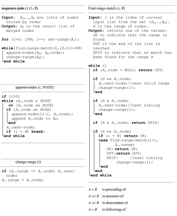
3.3. Algorithm of Sequence Join
The text of the algorithm is presented in Figure 7. The steps of finding match of the ranges and
appending result nodes are presented as separate sub-routines.
The algorithm generates the result list in the tree representation. To generate tuple represen-tation the append subroutine should iterate over the range nodes producing each possible com-bination.
The algorithm uses recursive subroutines. The depth of the recursion is equal the number of input lists which, in its turn, is related the depth of the input XML data tree. The depth of the existing XML databases does not exceed 20 and recursion will not cause consumption of mem-ory resources.
3.4. Time Cost Estimation
In this section we estimate the execution time difference between the proposed join algorithm and the pair-wise join algorithm. As there are multiple ways to break and n-way join into n binary joins, and the decision is chosen at run time, we assume that it is performed sequen-tially and all intermediate results are materi-alised.
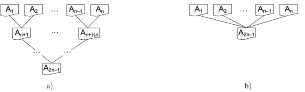
Consider regular path expressiona1/a2/:::/an. Both approaches require n selection operators resulting in lists of nodes A1 A2::: An re-spectively. The execution plans for pair-wise join and sequence join are shown in Figure 8 a) and b)accordingly. We consider the total time to perform join operation as the sum of time needed to read input lists (σ)and time neces-sary to create output list(τ): σ +τ.
For pair-wise approach, the task of matching complex query is reduced to performing of one join operation for each binary structural rela-tionship in query expression. Forn input lists of nodes, it causes creation of n2 intermediate lists of nodes. The next step is to perform bi-nary join operation over the intermediate lists. It is applied until it results in the only one, result list. Thus, the whole number of intermediate list
(including the result list)is
n
2+
n
4+:::+
n
2logn = 1;
1 2logn
n=n;1. In Figure 8 a)these lists are denoted as An+1
::: A2n
;1. If τi is the time required to create listi, then the total time necessary for creation of intermediate lists is 2n;1
P
n+1
Fig. 7. Sequence join algorithm.
The total number of list used as an input includes all the lists except the result one: n+
n
2 +
n
4 +
:::+
n
2(logn);1
= 2;
2 2logn
n=2(n;1). Ifσi is the time required to read listi, then the time necessary for reading of input lists is2n
;2 P
1 σi.
The total time necessary to perform multiple pair-wise join is
2n;2 X
1 σi+
2n;1 X
n+1
τi (1)
a) b)
Fig. 8.Execution plans of multiple pair-wise join and sequence join.
and read listirespectively.
The sequence join reads input listsA1,:::,An and creates the only one, result list A2n;1, as shown in Figure 8 b). The total time necessary to perform sequence join is
n
X
1
σi+τ2n ;1
(2)
whereσiis the time required to read input lists,
and τ2n;1 is the time needed to create result table.
The time difference between the two approaches is
2n;2
X
1 σi+
2n;1 X
n+1
τi
!
;
n
X
1
σi+τ2n ;1
!
= 2n;2
X
n+1
σi+ 2n;2
X
n+1
τi
(3) where τi and σi is the time required to create
and read listirespectively.
The parametersτiandσidepend on the capacity
of the listi. If the number of nodes in each list
is comparable, then we can assume the times to create and read list are equal: 8i i =1:::n;
τi = τ. The time cost functions of the algo-rithms (1) and (2), as well as their difference
(3), can be represented in a simpler form: the time cost of multiple pair-wise join is
(2σ +τ)(n;1) (1a)
the time cost of sequence join is
(σn+τ) (2a)
and their difference is
(σ +τ)(n;2) (3a)
whereτandσis an average time required to cre-ate an output and read an input list respectively,
nis the number of original input lists.
The algorithm time cost graphs are presented in Figure 9.
The graph shows that the sequence join algo-rithm does better over the queries with 3 and more basic structural relationships.
4. Experimental Evaluation
We have conducted several experiments eva-luating the proposed algorithm. The tests in-volve both real-world and synthetic datasets. This section describes experimental testbed and presents the results of these experiments.
4.1. Experimental Setup
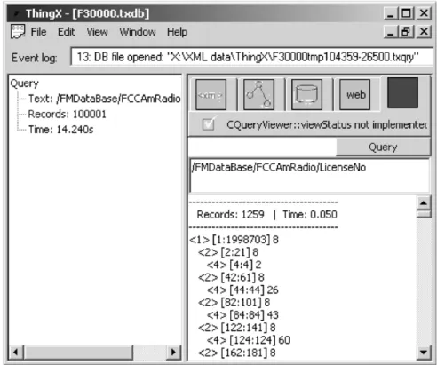
We implemented a prototype system for stor-ing, indexstor-ing, and querying XML data. The screenshot of the prototype window is shown in Figure 10. Source XML files are parsed using the Xerces-C++ XML parser 17]. The data is parsed without validation option. The proto-type exploits Berkeley DB 18] to store parsed data and index files. The B-tree indexing faci-lity of the package is used to build index files. The system provides a simple query interface for regular path expressions. The interface is XQuery-compliant 11] and directly performs query processing. The overall system is imple-mented in C++.
All experiments were performed under Win-dows 2000 workstation software running on a
Dell Dimension 8100 computer. The station has 256Mb of memory, 20Gb hard disk, and 1.4 GHz Pentium IV processor.
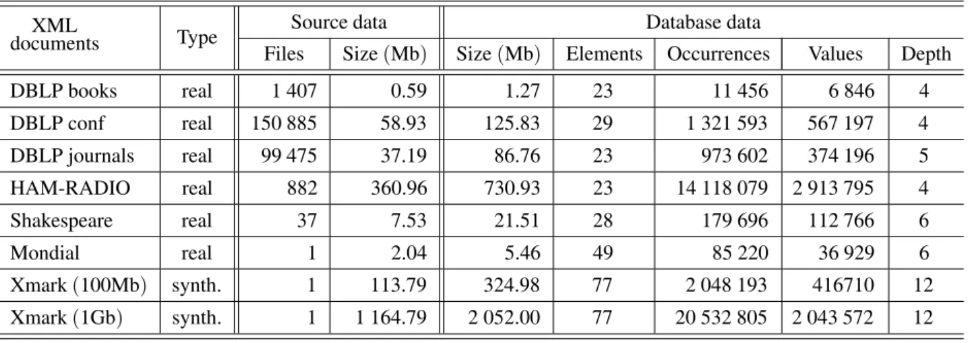
4.2. Data Sets
We have chosen several data sets, both real-world (DBLP 12], Shakespeare 13], HAM-RADIO 14], Mondial 15]), and synthetic
(Xmark 16]). The characteristics of these sources of data are summarised in Table 2. The columnsFilesandSizeof the Source data sec-tion show the number of the source XML doc-uments within the dataset and disk space occu-pied by them respectively. The field Size of the Database section refers to the size of the database obtained after parsing and storing the source documents. The Element column rep-resents the number of different element type names. It includes all the attribute names. The Occurrencesfield indicates the total number of element occurrences within the document and includes all attribute occurrences as well. The column Values show the total number of dif-ferent values of the elements. The fieldDepth show the maximum level of element nesting.
Source data Database data XML
documents Type Files Size
(Mb) Size(Mb) Elements Occurrences Values Depth
DBLP books real 1 407 0.59 1.27 23 11 456 6 846 4
DBLP conf real 150 885 58.93 125.83 29 1 321 593 567 197 4 DBLP journals real 99 475 37.19 86.76 23 973 602 374 196 5 HAM-RADIO real 882 360.96 730.93 23 14 118 079 2 913 795 4
Shakespeare real 37 7.53 21.51 28 179 696 112 766 6
Mondial real 1 2.04 5.46 49 85 220 36 929 6
Xmark(100Mb) synth. 1 113.79 324.98 77 2 048 193 416710 12
Xmark(1Gb) synth. 1 1 164.79 2 052.00 77 20 532 805 2 043 572 12
Table 2.Datasets characteristics.
A brief description of the data sets content is the following:
DBLPcontains computer science bibliogra-phy information 12]. It consists of many small files, each representing a single record about publication(conference or journal pa-per, book).
Shakespeare dataset is the XML version of the plays by Shakespeare13].
HAM-RADIOis the FCC Ham Radio data-base of the US Government’s Federal Com-munications Commission14].
Mondialis freely available geographic data-base15].
Xmarkdatasets are synthetic and were gen-erated by xmlgen generator 16]. The data
models an auction website with large num-ber of element and attribute types and high nesting of elements. We have selected stan-dard(100Mb)and large(1Gb)documents.
4.3. Queries and Performance Metrics
In order to study the tradeoffs of the join algo-rithm we carried out a series of comparative ex-periments. Query processing time was used as a major performance metric. The experiments evaluate the effect of several parameters on the performance of query processing: the size of the source XML files, number of elements and values, depth of the parsed tree, as well as the size of the query answer, number of elements
Records
# XQuery expression Dataset
Input Output %
RPE len
Q1 /book/isbn DBLP books 705 621 88% 2
Q2 /inproceedings/cite DBLP conf 214 837 102 519 48% 2
Q3 /article/author DBLP journals 245 748 245 216 99% 2
Q4 /FMDataBase/FCCAmRadio/Address/City HAM-RADIO 2115906 2115906 100% 3
Q5 /PLAY/ACT/SPEECH/LINE Shakespeare 139 083 138 620 99% 4
Q6 /country/province/city/name Mondial 26 032 6 616 25% 4
Q7
/person/profile/interest/category
Xmark(.1Gb) 309 588 97 176 31% 4
Q8 Xmark(1Gb) 1723670 977 538 57% 4
selected. The queries and their characteristics are given in Table 3.
We chose several test queries based on the length of the regular path expression and num-ber of matches. The column Input Records indicates the total number of processed records. The Output and “%” columns show the num-ber of records that match the query expression and their relative number against the processed records respectively. The RPE length repre-sents the length of the query expression path. If all single element subexpressions of the query expression are different, then this number coin-cides with the number of select operations for the query, i.e. the number of input lists.
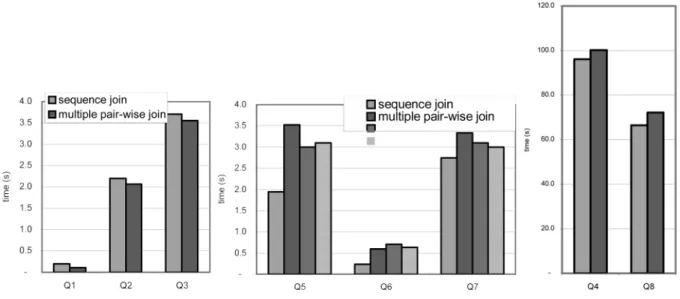
4.4. Experimental Results
The elapsed query time for the test datasets are shown in Figure 11. The cases with the query path length of more than 2(queries Q4– Q8)demonstrate improved performance of the sequence algorithm against the pair-wise algo-rithm.
The sequence join performs less effectively than the pair-wise join for the queries with the path length of 2(queries Q1–Q3). This fact is in ac-cordance with our time cost estimation shown in Figure 9.
For queries Q5-Q7, results are presented for different ways to break an n-way join into mul-tiple binary joins. Sequential join algorithm has
shown good performance against each of them. All the intermediate results for binary joins are materialised.
5. Conclusion
The structural join operation is intensely ex-ploited for finding structural patterns within an XML database. Thus, an effective implementa-tion of the structural join operaimplementa-tion is essential for effective XML query processing.
We have developed the sequence join algorithm for regular path expressions. In contrast to pair-wise approach, the algorithm takes several lists of elements as an input. It exploits the posi-tion of the element within XML document to compute structural relationships between ele-ments fast. The algorithm checks structural pattern matching through all the input lists at once. Due to this, it does not generate nonex-istent sub-results and hence eliminates creation of excessive intermediate data. Experimental evaluation of the algorithm shows that sequence join performs better than multiple binary joins for the queries with the expression length of 3 or more. It is true for the synthetic and real-world data queries of both small and large cardinality. As a direction for future activities, it is worth to consider sequence joins in context of graph-based queries. This area poses many interesting
problems, like handling graph-cycles (that are usually represented in the tree model as values of the link nodes). Another issue is process-ing the whole variety of XPath axes rather than ancestor-descendant or parent-child only.
6. Acknowledgements
This project is partly supported by ORS award. The authors would like to thank Jonathan Smith for his helpful comments on this paper.
References
1] D. SUCIU, On Database Theory and XML, in SIG-MOD record, v.30, n.3, September 2001.
2] S. AL-KHALIFA, H.V. JAGADISH, N. KOUDAS,
J.M. PATEL, D. SRIVASTAVA, AND Y. WU, Struc-tural Joins: A Primitive for Efficient XML Query Pattern Matching, Proceedings of the IEEE In-ternational Conference on Database Engineering (ICDE), 2002.
3] Q. LI, B. MOON, INDEXING AND QUERYINGXML DATA FOR REGULAR PATH EXPRESSIONS, Proceed-ings of the 27th VLDB Conference, Roma, Italy, 2001.
4] L. KRISHNA, J. HARITSA, SphinX: Schema-conscious XML Indexing, Technical report TR-2001-04, DSL/SERC.
5] S. ABITEBOUL, D. QUASS, J. MCHUGH, J. WIDOM, AND J. WIENER, The Lorel query language for
semistructured data,International Journal on Digi-tal Libraries, 1(1), pp. 68–88, April 1997.
6] C. ZHANG, J. F. NAUGHTON, D. J. DEWITT, Q. LUO,
G. M. LOHMAN, On Supporting Containment
Queries in Relational Database Management Sys-tems,Proceedings of the ACM SIGMOD Conference on Management Data, 2001.
7] A. DEUTSCH, M. FERNANDEZ, D. FLORESCU,
A. LEVY, D. SUCIU, A query language for XML, Computer Networks, 31(11–16), pp. 1155–1169,
Amsterdam, Netherlands, 1999.
8] T. BRAY, J. PAOLI, C.M. SPERBERG-MCQUEEN,
E. MALER, Extensible Markup Language (XML) 1.0 (Second Edition). W3C Recommendation, Technical report REC-XML-20001006. Available fromhttp://www.w3.org/TR/REC-xml, October 2000.
9] J. CLARK, S. DEROSE, XML Path Language (XPath) 1.0. W3C Recommendation, Tech-nical report REC-xpath-19991116. Available fromhttp://www.w3.org/TR/xpath, November 1999.
10] N.BRUNO, N.KOUDAS, D.SRIVASTAVA, Holistic
Twig Joins: Optimal XML Pattern Matching, Pro-ceedings of the ACM SIGMOD’02, 2002.
11] S. BOAG, D. CHAMBERLIN, M.F. FERNANDEZ,
D. FLORESCU, J. ROBIE, J. SIMEON´ , M. STE -FANESCU, XQuery 1.0: An XML Query Lan-guage. W3C working draft, Technical report WD-xquery-20020430, April 2002. Available from
http://www.w3.org/TR/xquery/.
12] DBLP.Computer Science Bibliography, Available
from http://www.informatik.uni-trier.de /ley/db/
13] J. BOSAK, The Plays of Shakespeare in XML.
Available from http://xml.coverpages.org /bosakShakespeare200.html.
14] HAM-RADIO. Available from ftp://ftp.
ictcompress.com/pub/xmltestfiles/.
15] W. MAY, Information Extraction and Integration with Florid: The Mondial Case Study, Techni-cal report 131, Universit¨at Freiburg, Institut f¨ur Informatik, 1999. Available from http://www. informatik.uni-freiburg.de/may/
Mondial/.
16] A. SCHMIDT, F. WAAS, M. KERSTEN, D. FLO -RESCU, I. MANOLESCU, M. J. CAREY, R. BUSSE, The XML benchmark project, Technical Report INS-R0103, CWI, April 2001. Available from
http://monetdb.cwi.nl/xml/Benchmark/ benchmark.html.
17] The Apache XML project. Xerces-C++ is a
validating XML parser. Available from http: //xml.apache.org/xerces-c/.
18] Berkley BD. Available from
http://www.sleepycat.com/.
Received:January, 2004 Accepted:June, 2004
Contact address: Oleksandr Logvynovskiy SCISM South Bank University 103 Borough Rd. SE1 0AA London, UK e-mail:[email protected] Kevin L¨u School of Business and Management Brunel University Uxbridge UB8 3PH, UK e-mail:[email protected]
ALEXANDERA. LOGVYNOVSKIYMSc in Computing and BSc in Com-puting. Currently, he is a PhD research student at London South Bank University, UK. His project is about semi-structured data management and mining.