Comparative Analysis of the Modified SOR and BGC Methods Applied to the Poleness Conservative Finite Difference Scheme

(1)

Vol. 6, No. 1, 2013, 30-43

ISSN 1307-5543 – www.ejpam.com

Comparative Analysis of the Modified SOR and BGC Methods

Applied to the Poleness Conservative Finite Difference Scheme

Arzu Erdem

Department of Mathematics, Kocaeli University, Umuttepe Campus, Izmit-Kocaeli, 41380, Turkey

Abstract. The poleness conservative finite difference scheme based on the weak solution of Poisson equation in polar coordinates is studied. Due to the singularity atr=0 in the considered polar domain

Ω_rϕ, a special technique of deriving the finite difference scheme in the neighbourhood of the pole point

r=0 is described. The constructed scheme has the order of approximation O

(h2_r+h2_ϕ)/r. In the second part of the paper the structure of the corresponding non-symmetric sparse block matrix is analyzed. A special algorithm based on SOR-method is presented for the numerical solution of the corresponding system of linear algebraic equations. The theoretical result are illustrated by numerical examples for continuous as well as discontinuous source function.

2010 Mathematics Subject Classifications: 65M06, 65F50, 65F10

Key Words and Phrases: Finite difference method, elliptic problem, polar coordinates, sparse matrix

1. Introduction

In this paper we consider the following Dirichlet problem for the Poisson equation in polar coordinates(r,ϕ):

  

Au:=₋1

r

∂ ∂r

r∂_∂u_r− _r12

∂2_u

∂ ϕ2 =F(r,ϕ), (r,ϕ)∈ΩR,

u(R,ϕ) =0, (r,ϕ)_∈Γ_ϕ,

u(r, 0) =u(r,β), r ∈(0,R),

. (1)

where Ω_R := _{(r,ϕ) _∈ R2 : r ∈ [0,R), ϕ _∈ [0,β)_}, Γ_ϕ := _{(R,ϕ) : ϕ _∈ [0,β)_}, and

β∈(0, 2π].

This problem is a mathematical model of various physical and engineering problems aris-ing in steady state flow of an incompressible viscous fluid in a duct of circular cross-section

[15, 13], in the determination of a potential in electrostatics[3]and in the elasticity theory

[8]. The two circumstances may lead to singularities: the geometrical singularity related to

Email address:erdem.arzugmail.om

(2)

the cornerβ∈(0, 2π)of the polar domain and the pole pointr=0. The first type of singular-ity means that for some values of the parameterβ∈(0,π)the second (and higher) derivative of the solutionu(r,ϕ)with respect tor∈[0,R)is singular atr=0. As show examples below the regularity of the weak solutionu∈H2(Ω)∩H1(Ω)of problem (1) depends on the value of the angle β ∈(0, 2π). This behaviour is usual for second order elliptic problems and is related to theC2-regularity property of the boundary∂Ω_R_βof the considered domain[1, 11]. The singularity at the re-entrant corner makes the numerical solution of these problems chal-lenging. The second type of singularity is a reason of many difficulties in constructing the standard finite difference (FD) schemes, when the pole r =0 is treated as a computational boundary. To avoid these difficulties various FD and pseudo-spectral (PS) methods have been suggested in literature[see 4, 14]. These schemes include the necessity of special boundary closures, which leads to undesirable clustering of grid points in PS schemes[see 4, 6]. The treatment of the singularities related to the situations r →0 and sinϕ_→0 have been given in[9, 10].

This paper is devoted to fill in the lack of result for conservative finite difference scheme for problem (1) and nonsymmetric sparse block matrices related to finite difference equations in polar coordinates. We present a conservative finite difference scheme for this problem and prove its convergence. Our approach is based on the Lax-Wondroff theorem[7], which guarantees convergence of a conservative FD schemes in the class of weak solutions, as the polar mesh is refined. Note that a similar technique was used in[12]for problem (1), where the classical solution of the boundary value problem (1) is considered. Since we are interested in bounded weak solutionsu∈H1(Ω_R), we require that the solution of problem (1) satisfies the boundedness atr =0 condition

lim

r→0r

∂u

∂r =0. (2)

Hence one needs to approximate not only the elliptic equation (1), but also condition (2). This condition will be used for obtaining the conservative finite difference scheme in the neighbourhood of the pole pointr=0.

Further, the FD approximations of problem (1)-(2) lead to large sparse system of linear equations, with the special nonsymmetric matrix, due to the periodicity condition

u(r, 0) = u(r,β). These type of linear systems require time-consuming algorithms for their effective numerical solution [2, 5]. We use the special structure of the obtained matrix[5]

and construct a fast iteration algorithm, based on SOR-method.

(3)

2. The Weak Solution and its Regularity Depending on the Parameter

β

∈

(

0, 2

π

)

Let v∈H1(Ω_R_β)be an arbitrary function, where

H1(Ω_R_β):=_{v∈H1(Ω_R_β):u(R,ϕ) =0,ϕ_∈(0,β); u(r, 0) =u(r,β), r∈(0,R)_} andH1(Ω_R_β)is the Sobolev space of functionsv=v(r,ϕ)with the norm

kuk₁:=   

Z Z

ΩRβ

u2+|∇u|2r d r dϕ

  

1/2

.

Let us multiply the both sides of equation (1) to r v(r,ϕ),r ∈(0,β)and integrate onΩ_R_β:

−

Z Z

ΩRβ

∂ ∂r

r∂u

∂r

+1 r

∂2u

∂ ϕ2

vd r dϕ= Z Z

ΩRβ

F(r,ϕ)v r d r dϕ.

Applying here by part integration, using the boundary and periodicity conditions (2) we get Z Z

ΩRβ

∇u(r,ϕ)· ∇v(r,ϕ)r d r dϕ= Z Z

ΩRβ

F(r,ϕ)v r d r dϕ, ∀v∈H1(Ω_Rβ). (3)

Here_∇uis the gradient vector in polar coordinates,

∇u= ∂u

∂re1+ 1 r

∂u

∂ ϕe2,

e1

e2

=

C osϕ, Sinϕ

Sinϕ, C osϕ

i1

i2

,

andi₁,i₂are unit coordinate vector in Cartesian coordinates. The solutionu∈H1(Ω_R_β)of the integral identity (3) is defined as a weak solution of the boundary value problem (1)-(2).

The integral identity (3) shows that if the functionu∈C2(Ω_R_β)_∩C1(Ω_R_β)is the solution of the boundary value problem (1)-(2), then for allv∈H1(Ω_R_β)this identity holds. Hence the weak solution of problem (1)-(2) can be defined as functionu∈H1(Ω_Rβ)satisfying this inte-gral identity for all v∈H1(Ω_R_β). According to the general theory for linear elliptic boundary value problems the regular weak solution of problem (1)-(2) belongs to H2(Ω_R_β)∩H1(Ω_R_β), if the boundary∂Ω_R_β is of classC2[4, 11]. The following example shows that depending on the valuesβ∈(π, 2π)of the parameterβ the weak solution of the boundary value problem (1)-(2) may not belong to the classH2(Ω_R_β).

Example 1. The function

u(r,ϕ) =rπ/βSin(πϕ/β), (r,ϕ)_∈Ω_R_β (4) satisfies the Laplace equation in polar coordinates and the Dirichlet condition

(4)

This function belongs to the Sobolev space H2(Ω_Rβ)∩H1(ΩRβ), for allβ ∈(0,π). However for

the valuesβ ∈(π, 2π)this solution doesn’t belong to H2(Ω_R_β), since rα ∈/ H2(Ω_R_β)forα <1. The reason, as shown in[11], is that forβ _∈(π, 2π)the boundary∂Ω_R_β doesn’t belong to the class C2, as requires the Agmon-Nirenberg regularity theorem[1].

Note that the above loss of regularity of the boundary∂Ω_R_β is a result of the introduced angle α=πϕ/β. When the parameter β changes in(0, 2π)the angleα always remains in (0,π). This also implies that for the functionu(r,ϕ), given by (4), the periodicity condition

∂u(r, 0)

∂ ϕ =

∂u(r,β)

∂ ϕ , r ∈(0,R) (5)

doesn’t hold. The next example shows that by introducing the parameterα=nπϕ/β,n=2, the fulfilment of this condition can be achieved.

Example 2. Consider now the function

u(r,ϕ) =r2π/βSin(2πϕ/β), (r,ϕ)∈Ω_R_β, (6) which evidently belongs to H2(Ω_Rβ), ∀β ∈(0, 2π). This function satisfies the Laplace equation

and the boundary conditions(1). Observe that the angleα=2πϕ/β always remains in(0, 2π), when the parameterβ changes in (0, 2π). This moment removes the lack of smoothness of the boundary and as a result the solution u(r,ϕ)∈H2(Ω_Rβ)∩H1(ΩRβ),∀β ∈(0,π), given by (6),

also satisfies the periodicity condition(5).

These two solutions show the main distinguished features of the boundary value problem (1)-(2), and they will be used for testing of the presented finite difference scheme.

3. The Conservative FD Scheme on a Piecewise Uniform Polar Mesh

We assume here β = 2π and introduce the following uniform meshes with respect to variablesr andϕ

wr:={rn= (n−0.5)hr:n=1, 2, . . . ,N+1, hr= (2R)/(2N+1)},

w_ϕ:=_{ϕm= (m−1)hϕ: m=1, 2, . . . ,M+1, hϕ=2π/M},

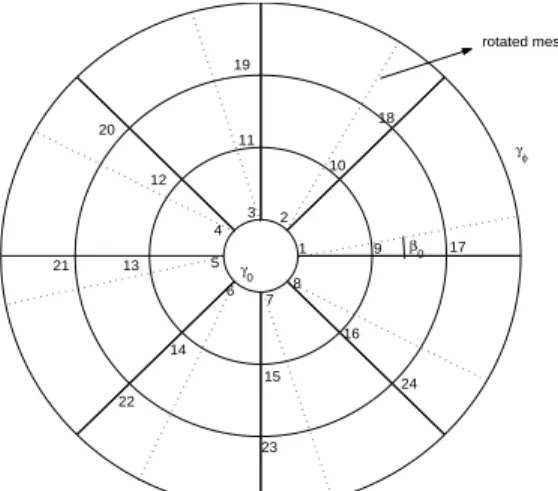
with mesh stepsh_r,h_ϕ >0. Then we obtain the piecewise uniform polar meshw_r_ϕ:=w_r×w_ϕ (Fig. 1):

w_r_ϕ:={(r_n,ϕm)∈ΩRϕ:rn∈wr, ϕm∈wϕ}, dimwrϕ= (N+1)×(M+1),

where wrϕ := wrϕ∪cγϕ∪γ0, and wrϕ := {(rn,ϕm) ∈ ΩRϕ : n = 2,N, m = 2,M}. The boundary mesh points are defined as follows

(5)

1 2 3 4

5

6 ₇ 8 10 11 12 13 14 15 16 9 18 19 20 21 22 23 24 17 β₀ γ₀ γ_φ rotated mesh

Figure 1: Geometry of the poleness polar mesh and its rotated form Due to the periodicity conditionu(r, 0) =u(r, 2π)we will not include the values

u(r, 0), r ∈ [0,R] to the list of unknowns in the discrete problem. The introduced mesh w_rϕ doesn’t include the pole pointr =0, that is in the presented discrete model the domain

Ω_R_ϕ is approximated by the circular disc ΩoRϕ. Thus our discrete model does not deal with the singularity at r =0, that is usual for the differential problem. Instead we will derive an approximation of the boundedness condition (2) at the central circle with radius

r=r1, r1=0.5hr.

Denote bye_nm={(r,ϕ)∈Ω_Rβ :rn≤r ≤rn+1, ϕm≤ϕ≤ϕm+1}the polar finite element

with four nodes. We derive an error approximation for each element. Introducing the half-nodes r_n± = rn±hr/2, ϕ±m =ϕm±hϕ/2 and integrating equation (1) on the finite element e

e_nm:= [r_n−,r_n+]×[ϕ−_m,ϕ_m+]we obtain the following balance equation: Z ϕ+

m

ϕ−_m Z r+

n

r_n− ∂ ∂r

r∂u

∂r

d r dϕ+ Z r+

n

r_n−

Z ϕ+ m

ϕ−_m 1 r

∂2_u

∂ ϕ2dϕd r=−

Z r+ n

r−_n

Z ϕ+ m

ϕ−_m

r F(r,ϕ)dϕd r. (7)

Let us transform the first left integralI_nmr .

I_nmr = Z ϕ+_m

ϕ−_m

r∂u

∂r r=r_n+

r=r_n−

dϕ∼=hϕ

r∂u

∂r

(r_n+,ϕm)−

r∂u

∂r

(r_n−,ϕm)

We use here the central finite difference formula for approximation of derivatives on the right hand side, by using the mesh points r_n, r_n₊₁_/₂, r_n₊₁, with mesh steph_r_/₂=h_r/2:

r∂u

∂r

(r_n+,ϕm) ∼= rn+

u(r_n₊₁,ϕm)−u(rn,ϕm)

h_r ,

r∂u

∂r

(r_n−,ϕm) ∼= rn−

u(r_n,ϕ_m)₋u(r_n₋₁,ϕ_m) hr

(6)

Then we have the following variational finite difference approximation of the integral operator I_nmr :

I_nmr ∼=hϕ

r_n+u_r,nm−rn−ur,nm

.

By the same way we can derive an approximation of the second integral operator Inmϕ on the

left hand side of (7):

Iϕ_nmu ∼= hr r_n

∂u

∂ ϕ(rn,ϕ + m)−

∂u

∂ ϕ(rn,ϕ

−

m)

∼

= hr r_n

uϕ(rn,ϕm)−uϕ(rn,ϕm)

.

Applying to the right hand side of (7) the numerical integration (rectangle) formula, finally we have

−hϕ[rn+yr,nm−rn−yr,nm]−

h_r

r_n[yϕ,nm− yϕ,nm] =hrhϕrnF(rnϕm)

Dividing byhrhϕrn>0 we obtain the following finite difference equation

Anmu:=−

₁ r(r yr)

r,nm

−

₁ r2yϕϕ

nm

=F(r_n,ϕm), (rn,ϕm)∈ωrϕ, n6=1. (8)

The finite dimensional operators

Ar

nmy :=

₁ r(r yr)

r,nm

, A_nmϕ y ₁

r2yϕϕ

nm

are the finite difference approximations of the differential operators

Aru:= 1 r

∂ ∂r

k(r)∂u

∂r

, Aϕu:= 1 r2

∂2u

∂ ϕ2, (r,ϕ)∈ΩRβ,

correspondingly. Note that the same approximations can also be obtained from the direct finite difference approximation of the Poisson equation (1).

The finite difference equation corresponding to the layer r=r₁=h_r/2 can be derived by using the same balance equation (7), substituting r_n−=ǫ, r_n+=h_r:

Z ϕ+ m

ϕ−_m Z hr

ǫ

∂ ∂r

r∂u

∂r

d r dϕ+ Z ϕ+

m

ϕ−_m Z hr

ǫ 1 r

∂2_u

∂ ϕ2d r dϕ=−

Z ϕ+ m

ϕ−_m Z hr

ǫ

r F(r,ϕ)d r dϕ.

Going to the limitǫ→0 here and using condition (2) we obtain Z ϕ+

m

ϕ−_m

∂u(h_r,ϕ)

∂r dϕ+ Z hr

0

1 r

∂u(r,ϕ+_m)

∂ ϕ −

∂u(r,ϕ−_m)

∂ ϕ

d r+

Z hr

0

r Z ϕ+

m

ϕ−_m

(7)

Again using the numerical integration formula in the first integral we get

h_rh_ϕ∂u(hr,ϕm)

∂r +2

∂u

∂ ϕ

h_r

2,ϕm+ hϕ

2

− ∂u

∂ ϕ

h_r

2,ϕm− hϕ

2

+h

2

rhϕ 2 F

_h

r

2,ϕm

≈0

To derive this finite difference equation in canonical form we use the standard definitions yr,1m:=

1

h_r[y(r1+hr,ϕm)− y(r1,ϕm)], yϕ,1m:=

1 hϕ

[y(r₁,ϕm)− y(r1,ϕm−1)],

yϕ,1m:=

1 hϕ

[y(r₁,ϕm+1)−y(r1,ϕm)].

Then we have

h_rhϕyr(r1,ϕm) +2hϕyϕ,ϕ(r1,ϕm) +

h2_rhϕ

2 F(r1,ϕm) =0, m=1, 2, . . . ,M

Dividing the both sides toh2_rhϕ/2 finally we obtain the finite difference equation correspond-ing to the layerr1=hr/2:

−_h2

r

yr(r1,ϕm)−

4

h2_ryϕ,ϕ(r1,ϕm) =F(r1,ϕm) =0, m=1, 2, . . . ,M. (9) Equations (8)-(9) represent the finite difference analogue of the Poisson equation (1) in the constructed polar meshωrϕ.

Lemma 1. If u ∈ C4(Ω_Rβ) then the order of the approximation error of the finite difference

schemes(8)-(9)in C-norm isψrϕ :ψrϕ =O

(h2_r+h2_ϕ)/rn

, where

ψrϕ=

h2_r 6r_m

 ∂

3_u

∂r3 +

r_n+h_r/2 4

∂4u(_er_n,ϕm) ∂r4 +

r_n−h_r/2 4

∂4u(e_er_n,ϕ)

∂r4  + h

2

ϕ 12r_m

∂4u(r_n,ϕ_em) ∂ ϕ4 .

(10) The explicit form (10) ofψ(h_r,ϕ_m)and the proof of this result is given in[11].

The lemma shows that as r →r₁ the functionψrϕ increases, and at the first layerr =r1

(r1=hr/2) becomesψrϕ=O(hr+h2ϕ/hr).

Note that the boundedness condition (2) is necessary for the above approximation, and hence for the convergence of the finite difference schemes (8)-(9), although this condition is not used explicitly on deriving the approximation error. To show this, consider the following: Example 3. The function

u(r,ϕ) =ln1

(8)

satisfies the Poisson equation (1) in Ω_Rβ, with for R = 1, β = 2π, and the right hand side

F(r,ϕ) = 1

r2 Sinϕ. Evidently this solution also satisfies the boundary and periodicity conditions

(1), but does not satisfy the boundedness condition(2), since r∂u/∂r =Sinϕ _6→0, as r →0. Calculating the right hand side of (10)for n=1we obviously observe that for r=r₁

ψ(r₁,ϕm) =

h2_ϕ

12r₁3sinϕm.

This shows thatψ(r₁,ϕm)6→0, as r1→0, and there is no approximation in the neighbourhood

of the pole point r=0.

To formulate the discrete problem we need to add to equations (8)-(9), the equations, obtained from the periodicity condition (1).

4. The Algebraic Problem with Nonsymmetric Sparse Matrix: Iteration

Algorithm

The finite difference equations (8)-(9) compose K:=N Mnumber of algebraic equations withK unknowns

y= (y₁₁, y₁₂, . . . , y₁_M, y₂₁, . . . , y_{N M})T, dimy=K.

We can rewrite these equations in the form of the system of linear algebraic equations

Ay=F with the following positive band matrixA, dimA =K×K:

A :=

         

A11 A12 0 0 . . . 0 0 0

A₂₁ A₂₂ A₂₃ 0 . . . 0 0 0

0 A₃₂ A₃₃ A₃₄ . . . 0 0 0

. . . .. . . . 0 0 0 0 . . . A_N₋_1,_N₋₂ A_N₋_1,_N₋₁ A_N₋_1,_N 0 0 0 0 . . . 0 AN,N−1 AN,N

          .

HereM×M-dimensional block matricesA_{i j} are of the following structure:

Aii=

         

• • 0 0 . . . 0 0 •

• • • 0 . . . 0 0 0

0 • • • . . . 0 0 0

. . . .. ... ... ...

0 0 0 0 . . . • • •

• 0 0 0 . . . 0 • •

         

and

(9)

The parametersαiandβican be defined from the finite difference schemes (8)-(9) as follows: α1=

2

h2_r; αi = k_i

rih2r

, i=2,N; βi =

k_i+1

rih2r

, i=1,N.

Sinceαi 6=βi, the matrix A is not symmetric one. Moreover, A is a sparse matrix of

spe-cial structure, corresponding to the polar mesh and periodicity condition. Evidently such a system of linear algebraic equations with non-symmetric sparse matrix needs to be solved by iteration methods[12, 13, 14]. However, as the computational experiments below show, use of compact storage for the band matrixA and then an application of any effective iteration method requires large enough time for the solution of the linear system of algebraic equations

Ay=_F. The reason is that the bandwidth of the non-symmetric matrixA is bw=3M

and there are many null terms in the band. Specifically, the above block matricesA_ii,A_ii₊₁, Ai−1i containM2−3M, M2−M, M2−M zero elements, correspondingly. Hence forM =N

the number of zero and non-zero elements of the band are 3N3−4N2−4N and 5N2+N, respectively. For the mesh withN =30, this means that the number of non-zero elements of the band matrix A is about 4.3% of all band elements. Therefore one needs to construct a special algorithm which can store and operate with only nonzero elementsαiandβi, realising

the multiplicationsU y and L y, to minimize the time required for the solution of the consid-ered problem by any iteration method. Here theU andL are the upper and lower triangular matrices:A =D+U+L. Note that for some class of systems, arising from the finite-element discretization, similar algorithm was constructed in[15].

Table 1 illustrates the comparative analysis of the standard SOR method

yk+1= (D+ωL)−1[(1₋ω)D₋ωU]yk+ω(D+ωL)−1_F, (11) by using MATLAB code, and SOR method with the constructed here special algorithm. As a test example the analytical solution given in Example 2, withβ =2π, is used. The iteration parameterω∈(0, 2)in (11) was defined by the formula

ω= 2

1+pλ_min(2−λ_min),

whereλ_min is the minimal eigenvalue of the Laplace operator, andλ_min =2sin2(π/2N), for the square meshM =N.

(10)

Table 1: Comparison of the standard and modified SOR algorithms N×M SOR with special algorithm Standard SOR Condition number

CPU time(sec.) CPU time(sec.) of the matrixA

20×20 0 9 1.5×104

30_×30 0 48 8.0_×104

40×40 0 126 2.5×105

5. Numerical Solution of the Elliptic Problem

(1)

-

(2)

by the Poleness

Conservative Schemes

(8)

-

(9)

In this section we discuss results of computational experiments related to numerical so-lution of the Dirichlet problem (1)-(2) by the poleness conservative scheme (8)-(9). In the first series of the computational experiments, the convergence and accuracy of the numerical solution of the Dirichlet problem (1)-(2), with the analytical solution

u(r,ϕ) = (r₋1)Sinϕ, (r,ϕ)_∈Ω_R_β, R=1, is studied. Note that the corresponding source function

F(r,ϕ) = 1

r2 Sinϕ, (r,ϕ)∈ΩRβ, (12)

has singularity at r = 0. The two appropriate iterative methods - SOR method and Bi-Congugate Gradient (BCG) method - are applied for the iterative solution of the linear system of algebraic equations, corresponding to the finite difference schemes (8)-(9). In all cases the MATLAB codes of this methods with the above mentioned special algorithm is used. Results are presented in the Table 2. For the comparison, the numerical results obtained by the Gauss-Seidel method, are also presented. Here and below the value of the stopping parameterδ >0 in

kuni−1−_unik 0≤δ,

wherek · k0is the L2-norm, is takenδ=10−5.

Table 2 shows numbers of iterations corresponding to all three iteration methods, with H1-relative and L_∞-absolute errors. Results given in the table show that for relatively coarse meshes BGC method is more effective than the SOR method. But for the meshes 45×45 and higher, SOR method is more effective in the sense of iterations. Moreover, the number of iterations n_i in SOR method increases slowly, as increases the number of mesh points. Thus ni =234 and ni =277, for the meshes 40×40 and 50×50, respectively. As show the last

three columns of the table, theH1-relative andL_∞-absolute errors are small enough, although the source function (12) has singularity at the pole pointr=0.

The next series of computational experiments is realized for the smooth continuous source function

˜

F(x,y) =F(r,ϕ) = (

50e x p(₋ ǫ2

ǫ2₋_r2), 0<r< ǫ

(11)

Table 2: Comparative analysis of the modified SOR and BGC methods applied to the poleness conservative finite difference scheme (8)-(9)

Methods N×M Time Number of Rel. error Abs. error Abs. error (sec.) iterations H1-norm L_∞-norm L_∞-norm

n_i r=r1 r=R/2

30×30 0 185 8.0×10−6 3.8×10−3 1.3×10−3 SOR 40×40 1 234 2.7×10−6 2.5×10−3 8.1×10−4 50×50 2 277 1.4×10−6 1.9×10−3 5.9×10−4 30×30 0 110 8.0×10−6 3.4×10−3 1.2×10−3 BCG 40×40 2 224 2.5×10−6 2.0×10−3 6.8×10−4 50×50 4 385 1.0×10−6 1.3×10−3 4.3×10−4 30×30 33 473 8.5×10−6 4.9×10−3 1.2×10−3 Gauss- 40×40 95 762 5.0×10−6 3.0×10−3 7.8×10−4 Seidel 50×50 219 1105 1.1×10−5 2.0×10−3 1.6×10−3 withǫ=1/2, approximating in weak sense the Diracδ-function (Figure 2a). This function is taken as a given data for the Dirichlet problem (1)-(2). The right pane, Figure 2b, illustrates the numerical solution ˜u_h(x,y) = u_h(r,ϕ) of problem (1)-(2) by the poleness conservative schemes (8)-(9), for the mesh size 30×30.

Finally we consider the weak solution of the Dirichlet problem (1)-(2), when the source F(r,ϕ)is a discontinuous atr=1/2 function

˜

F(x,y) =F(r,ϕ) =   

50ǫe x pp(−ǫ2/4r)

4πr3 , 0<r< ǫ

50ǫe x pp(−ǫ2/4)

4π , ǫ <r <R, R=1,

given in the left pane of Figure 3. This function with ǫ = 1/2 is taken as a given data for the Dirichlet problem (1)-(2). The numerical solution ˜uh(x,y) = uh(r,ϕ) of problem

(1)-(2) obtained for the mesh 30×30 is plotted in the right pane, Figure 3b. To estimate an accuracy of the numerical solution, in particular at the discontinuity point r = 1/2, the numerical solutionsu(1)_h (r,ϕ) =u(2)_h (r,ϕ)corresponding to two different meshesw(1)_r_ϕ =w(_r2_ϕ) is compared. The relative error

ǫh=

u(1)_h (r,ϕ)₋u(_h2)(r,ϕ) 0.5u(1)_h (r,ϕ) +u(_h2)(r,ϕ)

∞

,

is aboutǫh=10−3÷10−3, including the discontinuity point. This shows high accuracy of the

(12)

(a) Continuous Source Solution (b) Numerical Solution

Figure 2: Dirichlet problem in polar coordinates

(a) Discontinuous Source Solution (b) Numerical Solution

(13)

6. Conclusion

We studied poleness conservative finite difference scheme for Laplace operator in polar coordinates. The scheme with the modification of the SOR method allows to construct an effective numerical method for solving the Dirichlet problem in the polar coordinates, based on the weak solution approach. Numerical results presented for discontinuous source function shows high accuracy of the method on acceptable meshes.

Extension of results given here can be made for positive elliptic operators with discontin-uous coefficients, and for nonlinear monotone operators of Plateau type, as well. This require some additional techniques that will be done in next studies.

References

[1] S. Agmon, A. Douglis, and L. Nirenberg.Estimates near the boundary for solutions of ellip-tic partial differential equations satisfying general boundary conditions. Communications on Pure and Applied Mathematics.17, 35-92. 1964.

[2] A.M. Bruaset.A Survey of Preconditioned Iterative Methods. Addison-Wesley. 1995.

[3] J.D. Jackson.Classical Electrodynamics. 2nd Ed., Wiley, New York. 1975.

[4] M.D. Griffin, E. Jones, and J.D. Anderson.A computational fluid dynamic technique valid at the centerline for non-axisymmetric problems in cylindrical coordinates. Journal of Com-putational Physics.30, 352-364. 1979.

[5] W. Hackbush. Iterative Solution of Large Sparse Systems of Equations. Springer-Verlag, Berlin. 1994.

[6] W. Huang and D.M. Sloan.Pole condition for singular problems: The pseudo-spectral ap-proximation. Journal of Computational Physics.107, 254-365. 1993.

[7] P.D. Lax and B. Wendroff.Systems of conservation laws. Communications on Pure and Applied Mathematics.13, 217-237. 1960.

[8] A.I. Lurie.Three-Dimensional Problems of the Theory of Elasticity. Interscience Publishers, New York. 1964.

[9] P.E. Merilees.The pseudospectral approximation applied to the shallow water equations on a sphere. Atmosphere,13(1), 897-910.1973.

[10] K. Mohseni and T. Colonius.Numerical treatment of polar coordinate singularities. Journal of Computational Physics.157, 787-795. 2000.

(14)

[12] A.A. Samarskii and V.B. Andreev. Difference Methods for Elliptic Problems (in Russian). Nauka, Moscow. 1976.

[13] F.S. Sharman.Viscous Flow. McGraw-Hill, New York. 1990.

[14] R. Verzicco and P. Orlandi.A finite difference scheme for three dimensional incompressible flows in cylindrical coordinates. Journal of Computational Physics.123, 402-415. 1996.