Vol. 5, No. 3, 2012, 282-301
ISSN 1307-5543 – www.ejpam.com
Performance of Information Complexity Criteria in Structural
Equation Models with Applications
Eylem Deniz Howe
1,∗, Hamparsum Bozdogan
2, and Gülay Kıro˘
glu
11Mimar Sinan Fine Arts University, Istanbul Turkey
2 Department of Statistics, Operations, and Management Science, The University of Tennessee,
Knoxville, TN, 37996, USA
Abstract. A common problem in structural equation modeling is that of model selection. Many re-searchers have addressed this problem, but many methods have provided mixed benefits until recently. Akaike’s well-known criteria,AI C, has been applied in the context of structural equation modeling, but the effectiveness of many other information criteria have not been studied in a convincing manner. In this paper, we compare the SEM model selection prowess of severalAI C-type andI COM P-type crite-ria. We also introduce two new large sample consistent forms of Bozdogan’sI COM P criteria - one of which is robust to model misspecification.
To study the empirical performance of the information criteria, we use a well-known SEM simulation protocol, and demonstrate that most of the information-theoretic criteria select the “pseudo true” model with very high frequencies. We also demonstrate, however, that the performance of AI C is inversely related to the sample size. Finally, we apply the new criteria to select an analytical model for a real dataset from a retail marketing study of consumer behavior. Our results show the versatility of the new proposed method where both the goodness-of fit and the complexity of the model is taken into account in one criterion function.
2010 Mathematics Subject Classifications: 62H12,62H15,62H20,62H25,62P15,62F35
Key Words and Phrases: Structural Equation Model, Information Criteria,AI C-type Criteria,I COM P -type Criteria
1. Introduction
Structural Equation Modeling (SEM) has been a popular tool in social and behavioral sciences since the early 1990’s for the causal modeling of complex, multivariate data sets. Presently, it has penetrated engineering, management and information sciences, and genomic research, to mention a few. It has changed the perspective of researchers on how to do good statistical modeling and model selection. It has also fostered the curiosity of social
∗Corresponding author.
Email addresses:eylemdenizgmail.om(E. Howe),bozdoganutk.edu(H. Bozdogan),
gkiroglumsu.edu.tr(G. Kıro˘glu)
scientists about the underlying constructs or factors in many applications. According to[11], the SEM approach has been regarded, perhaps, as the most significant and effective statistical revolution in social sciences.
In SEM one of the fundamental problems is how to evaluate different models and how to select among the rival models[18]. In the literature of SEM, there are many alternative fit indices available to the researchers. An excellent recent book by [22], “Linear Causal Mod-eling with Structural Equations” devotes a fair amount of discussion on many goodness-of-fit indices. Mulaik [22]further discusses information theoretic measures of model discrepancy such as AIC, see, e.g.,[1, 2, 27, 4]. He devotes a section on the information theoretic mea-sure of complexity (ICOMP) developed in[6, 7]. However, [22]does not provide numerical examples or evaluate the empirical performance of these model selection criteria in the SEM framework.
The first author in [14], evaluated the performance of several information criteria for measurement models and SEMs. In this paper, our objective is to to extend that research and to present some new results on ICOMP which is consistent with respect to sample size and robustness against model misspecification in SEM and in other high dimensional model fitting.
Therefore, in this paper we revisit and discuss information criteria used to gauge model fit in structural equation modeling (SEM). This is based on the objective that statistical methods of fit are related to sample size, any statistical test is increasingly likely to imply rejection of a model as sample size increases, even if model misfit is trivial in magnitude. Various practical fit indices have been proposed over the years - and information criteria are among the most widely used. We review prior information criteria, and propose a couple of new information criteria based on information measure of complexity of a covariance matrix called I COM P -type criteria.
We demonstrate the empirical performance of I COM P-type criteria along withAI C, Con-sistent Akaike Information Criterion (CAI C), Consistent Akaike Information Criterion with Fisher Information (CAI C F) both due to [4], and a Bayesian Model Selection (BM S) crite-rion developed by[10].
2. Structural Equation Model with Latent Variables
General SEMs consist of two models referred to as measurement and structural equation (or latent variable) models. The structural equation model defines relationship between la-tent variables. This model is a path model adapted to lala-tent variables. The measurement model is a confirmatory factor (CF) model which defines relationship between observed and latent variables. Latent variables in the measurement model are the factors in the CF model. Following[19]in matrix notation, we define the general SEM model with these two models by three equations:
Structural Equation model: η (r×1)
= Bη
(r×r)(r×1)
+ Γξ (r×s)(s×1)
+ ζ (r×1)
Measurement model for y: y (p×1)
= Λyη (p×r)(r×1)
+ ǫ (p×1)
Measurement model for x: x
(q×1)=(q×Λs)(xsξ×1)+(qδ×1)
whereηis a(r×1)vector of latent endogenous (or dependent) variables,ξis(s×1)vector of latent exogenous (or independent) variables,ζis(r×1)vector of latent errors in equations,
β is an(r×r)coefficient matrix for the latent endogenous variables, and Γis a (r×s) co-efficient matrix for the latent exogenous variables. The structural model specifies the causal relationships among the latent endogenous variables in β, between the exogenous and en-dogenous variables inΓ, and describes unexplained residuals of the latent factors inζ. The usual assumptions for the structural model are that:
E(η) =E(ξ) =E(ζ) =0,ζis uncorrelated withξ, and(I−β)is nonsingular. The covariance matrix,
E(ξξ′) = Φ, (1)
is an(s×s)covariance matrix of the latent exogenous variables, and
E(ζζ′) = Ψ (2)
is an (r×r) covariance matrix of the latent errors in equations. The measurement model specifies how the observed variables, x and y, are determined through Λx and Λy by the latent variables, ξandη, respectively. Theǫandδ terms represent the residuals in x and y
unexplained byξandη. The usual assumptions for the measurement model are:
E(η) =E(ξ) =E(ǫ) =E(δ) =0 . Furthermore,ǫis uncorrelated withξ, ηandδ. Likewise,
δis uncorrelated withξ,η andǫ. The covariances matrices in the case of the measurement model are:
E(ǫǫ′) = Θǫ= Σ(ǫ), (3)
a(p×p)covariance matrix ofǫ, and
E(δδ′) = Θδ= Σ(δ), (4)
According to the measurement and structural equation models, the implied full covariance matrix,Σ(θ), for the general SEM is given by
Σ(θ) =
Λy(I−B)−1(ΓΦΓ′+ Ψ)[(I−B)−1]′Λ′y+ Θε Λy(I−B)−1ΓΦΛ′x
(Λy(I−B)−1ΓΦΛ′x)′ ΛxΦΛ′x + Θδ
. (5)
The elements of the general implied covariance matrix are functions ofB,Γ,Λy,Λx,Φ,Ψ,Θε
andΘδ. To be able to use SEM, we need to specify the pattern of the elements of these eight matrices. There are three kinds of specifications. These are:
• Fixed parameters- that have been assigned specific values,
• Constrained parameters- that are unknown but equal to one or more other parameters, and
• Free parameters- that are unknown and not constrained to be equal to any other pa-rameter.
For more on these, see[3, 19], and others.
The fundamental hypothesis for these structural equations procedures is that the covari-ance matrix of the observed variables is a function of a set of parameters. If the model is correct and if we know the parameters, then the population covariance matrix can be exactly reproduced. The hypothesis in this case is:
Σ = Σ(θ). (6)
In (6),Σis the population covariance matrix of the observed variables,θis a vector containing the free parameters of the model, andΣ(θ)is the covariance matrix written as a function of the covariance matrix implied by a specific model[3].
3. Information Theoretic Model Selection Criteria
One of the fundamental difficulties in statistical analysis and data mining is the choice of an appropriate model, estimating and determining the order or dimension of a model. In gen-eral statistical modeling and model evaluation problems, the concept of information theoretic measure of complexity plays an important role. At the philosophical level,complexityinvolves notions such as connectivity patterns and theinteractions of model components. Without a measure ofoverallmodel complexity,prediction of model behaviorandassessing model quality
is difficult. This requires detailed statistical analysis and computation to choose thebest fitting model among a portfolio of competing modelsfor a given finite sample[4].
Based on Akaike’sAI C, many model-selection procedures that take the form of apenalized likelihoodplus apenalty term) have been proposed.
For a general multivariate linear or nonlinear model defined by
a summary diagram for AIC and ICOMP in terms of aloss functionis give by
Loss= Lack of Fit
+Lack of Parsimony
«
−→ AI C
+Profusion of Complexity
−→ I COM P
3.1. Akaike-Type Information Criteria
Since Akaike (1973), entropic information criteria has had a substantial impact in statis-tical model evaluation problems. Its introduction furthered the recognition of the importance of good modeling and model fitting in the statistical science. As a result, many important statistical modeling techniques have been developed in various fields of statistics such as in biostatistics, control theory, econometrics, engineering, medical data mining, psychometrics, and many others.
Akaike Information Criterion (AIC)
AI C, which is one of the first information criterion developed by Akaike, can be thought of as a generalized form of the maximum likelihood. AI C can be formulated as maximizing generalized entropy, or equivalently minimizingKullback-Leibler (KL) information. See, e.g. [21], and [20]. It is obtained from asymptotic unbiased estimation of the logarithm of the average expected likelihood of a model and it is defined by
AI C=−2 logL(θbk) +2k, (8)
where θ is a k-dimensional unknown parameter vector,θb, denotes the maximum likelihood estimator ofθ, L(θb), is the maximized likelihood function of the model, andkis the number of unknown parameters estimated in the model.
Consistent Akaike Information Criterion (CAIC)
Without violating Akaike’s principles and using the results in mathematical statistics, Bozdo-gan [4] extendedAI C analytically in two ways. These extensions makeAI C asymptotically consistent, and penalize overparameterization more stringently, so as to pick the simplest of the true models whenever there is nothing to be lost in doing so. CAI C is defined by
CAI C =−2 logL(θbk) +k(log(n) +1). (9)
Consistent Akaike Information Criterion with Fisher Information (CAICF)
Also in[4], a different estimator for negative twice the expected entropy was proposed. Sim-ilar to CAI C, this approach extends AI C analytically to make it consistent without deviat-ing from Akaike’s original premise. In this manner[4]penalizes overparameterization more strongly, in particular, in large samples.CAI C F is defined by
CAI C F=−2 logL(θb) +k(log(n) +2) +log|F |ˆ, (10)
whereFˆis the estimated Fisher information matrix (FIM) of the model.
Bayesian Model Selection Criterion (BMS)
Bozdogan and Ueno [10] provided yet a further extension of AI C called Bayesian Model Selection Criterion (BM S), given by
BM S=−2 logL(θb) +klog(n) +2( nk
n−k−2) +log|F |ˆ. (11)
As we note, these extended formsAI C all attempt to repair the inconsistency problem of the
AI C.
3.2. The General Form of Information Complexity: ICOMP
Motivated from considerations similar to those inAI C, here we give details anew entropic or information-theoretic measure of complexitycalledI COM P of[6, 7, 9]as a decision rule for model selection in SEM.
The development and construction of I COM P is based on a generalization of the covari-ance complexity indexoriginally introduced in [29]. Instead of penalizing the number of free parameters directly, I COM P penalizes the covariance complexity of the model. It is defined by
I COM P=−2 logL( ˆθk) +2C(C ovÔ( ˆθk)), (12)
where L( ˆθk)is the maximized likelihood function,θˆk is the maximum likelihood estimate of
the parameter vectorθk under the modelMkwith kunknown parameter, andC represents a
real-valued complexity measure.
As explained in[7, 8, 9], there are several forms and theoretical justifications ofI COM P. For brevity, here, we will recapitulate and use one of the most general forms of I COM P
For a multivariate normal linear or nonlinear structural model we define the general form ofI COM P(I F I M)as
I COM P( ˆF−1) =−2 logL( ˆθk) +2C1( ˆF−1), (13) whereC1denotes the maximal informational complexity ofFˆ−1 and is given by
C1( ˆF−1) = s
2log[
t r( ˆF−1)
s ]−
1 2log|Fˆ
−1|, (14)
and wheres=d im( ˆF−1) =r ank( ˆF−1).
The first component of I COM P(I F I M) measures the lack of fit of the model, and the second component measures the complexity of the accuracy of the estimated parameters and implicitly adjusts for the number of free parameters included in the model. It is a measure of the state of disorder of a model for a given data set. For more on this, and for some immediate physical motivation, we refer the readers to the interesting book by[16], entitled
“Physics from Fisher Information.”
The trace of I F I M in the complexity measure involves only the diagonal elements anal-ogous to variances while the determinant involves also the off-diagonal elements analanal-ogous to covariances. Therefore,I COM P(I F I M) contrasts the trace and the determinant of I F I M, and this amounts to a comparison of the geometric and arithmetic means of the eigenvalues ofI F I M given by
I COM P( ˆF−1) =−2 logL( ˆθ
k) +slog
λa/λg
. (15)
We note that I COM P(I F I M) now looks in appearance like the CAI C, M D L [26], and the Bayesian criterion SBC [28], except for using logλa/λg
instead of using log(n), where log(n) denotes the natural logarithm of the sample size n. In this sense, I COM P(I F I M)
resembles a penalized likelihood method similar toAI CandAI C-type criteria, except that the penalty depends on the curvature of the log likelihood function via the scalarC1 complexity value of the estimatedI F I M.
3.3. Consistent and Misspecification Forms of ICOMP
Bozdogan [9] suggested several other different approaches to generalize and derive the
I COM P criteria by maximizing theposterior expected utility(PEU) when the models are mis-specified (which is the case in practice). Here, we give derived forms of these generalized
I COM Pcriteria as follows.
I COM PFˆ−1P E U_M iss=−2 logLθˆ+k+2t rFˆ−1Rˆ+C1Fˆ−1 (16)
In (16), whereasFˆ−1isI F I M in inner-product form,RˆisI F I M in outer-product form. If the model is correctly specified, these two forms of Fisher information matrices would be equal to one another. That is, ifFˆ−1= ˆR, then t r( ˆF−1R) =ˆ t r I
k
=k. In this case, we have
= AI C3+2C1( ˆF−1) (17) Bozdogan[9]approximates the term t r( ˆF−1R)ˆ in equation (16) by
t rFˆ−1Rˆ= nk n−k−2
which corrects the bias for small as well as large sample sizes. Thus, equation (16) reduces to
I COM PFˆ−1P E U_M iss=−2 logL( ˆθ) +k+2( nk
n−k−2) +2C1( ˆF
−1). (18)
This form ofI COM P is useful in cases where we cannot determine the closed form expression ofRˆ, outer-product form of I F I M in many modeling situations and SEM is a case in point example.
Consistent I COM P that maximizes theposterior expected utility(PEU)is given by
C I COM P( ˆF−1)P E U = −2 logL( ˆθ|X) +k+2klog(n) +2C1( ˆF−1)
= CAI C+2C1( ˆF−1). (19)
Further, consistentI COM Pthat maximizes theposterior expected utility(PEU) and also guards us against misspecification is given by
C I COM P( ˆF−1)P E U_M iss=−2 logL( ˆθ|X) +k+2 log(n) nk
n−k−2+2C1( ˆF
−1). (20)
A model with minimum ICOMP-type and AIC-type criteria are chosen to be the best model among all possible competing alternative models.
With I COM P-type criteria, complexity is viewed not as the number of parameters in the model, but as the degree of interdependence (i.e., the correlational structure among the pa-rameter estimates). By defining complexity in this way, I COM P-type criteria provide a more judicious penalty term thanAI C, M D L,SBC, orCAI C. The lack of parsimony is automatically adjusted by C1( ˆF−1) across the competing alternative portfolio of models as the parameter spaces of these models are constrained in the model selection process. For more onI COM P -type criteria, we refer the readers to[9]and[13].
4. Derived Forms of Information Criteria in Structural Equation Models
4.1. AIC-type Criteria in SEM
Under the assumption that the observed variables are continuous and have interval scales, and multivariate normal, that is,
z= (y′,x′)′∼N(p+q)(0,Σ(θ)) (21) and using the maximum likelihood estimators, we obtain AI C, CAI C, CAI C F and BM S for the SEM. These are given in[13]as follows.
CAI C=n(p+q)log(2π) +nlog|Σ|ˆ +nt r( ˆΣ−1S) +klog(n) +1, (23)
CAI C F=n(p+q)log(2π) +nlog|Σ|ˆ +nt r( ˆΣ−1S) +klog(n) +2+log|F |ˆ, (24)
BM S=n(p+q)log(2π) +nlog|Σ|ˆ +nt r( ˆΣ−1S) +klog(n) + ( nk
n−k−2) +log|F |ˆ, (25)
wherekis the number of parameters in SEM.
4.2. ICOMP-type Criteria in SEM
LetΣ( ˆˆ θ)denote the maximum likelihood estimator (MLE) of the implied covariance ma-trixΣ(θ)given by
ˆ Σ( ˆθ) (p+q)×(p+q)
=
ˆ
Λy(I−Bˆ)−1(ˆΓ ˆΦˆΓ′+ ˆΨ)(I−Bˆ′)−1Λˆy+ ˆΘǫ Λˆy(I−Bˆ)−1Γ ˆˆΦ ˆΛ′x ˆ
ΛxΦˆˆΓ′(I−Bˆ′)−1Λˆ′y ΛˆxΦ ˆˆΛ′x+ ˆΘδ
. (26)
The firstI COM P criterion in SEM is given by
I COM P=n(p+q)log(2π) +nlog|Σ|ˆ +nt r( ˆΣ−1S) +2C1( ˆΣ( ˆθ)). (27) We can also use the estimatedI F I M, the covariance of the model parameters, for the general SEM as given by
ˆ F−1=
1
nΣ( ˆˆ θ) 0
0′ 2n D (p+q)
+[ ˆΣ( ˆ
θ)⊗Σ( ˆˆ θ))] D (p+q)
+′
(28)
to obtain several other new forms ofI COM P based on the work of[5].
Note that in one dimension equation in (28) reduces to the I F I M of the normal distribu-tionN(µ,σ2)given by
ˆ F−1=
1
nσˆ
2 0
0′ 2nσˆ4
(29)
which checks and shows the correctness of the formula in (28) and thatθˆhas the consistency property.
In (28), the matrix D+p is the Moore-Penrose inverse of the duplication matrix Dp. The
duplication matrixDpis a uniquep2×12p p+1matrix, and so its Moore-Penrose inverse is
D+p =D′pDp
−1
D′p
which is a 1
2p p+1
×p2 matrix. Further, note that the duplication matrix Dp is implicitly defined by
Dpvech( ˆΣ( ˆθ)) =vec( ˆΣ( ˆθ))
wherevech( ˆΣ)vectorizes the distinct elements ofΣˆ by vertically stacking those on and below the principal diagonal. Consequently
Based on the above results, we establish I COM P(I F I M) for the SEM with latent variables given by
I COM P( ˆF−1) =n(p+q)log(2π) +nlog|Σ|ˆ +nt r( ˆΣ−1S) +2C1( ˆF−1). (30) We further note that with C1( ˆF−1), we do not actually need to constructFˆ−1, since it is a scalar measure of complexity. As derived in[13], using the definition of complexity, we get a computationally convenient open form of the expression forC1( ˆF−1)— in the sense that all the required inputs are available as a part of the standard output of most SEM packages — is
C1( ˆF−1) =
s 2log 1
nt r( ˆΣ) +
1 2n
t r( ˆΣ2) + (t r( ˆΣ))2+2
pP+q
j=1
ˆ σj j
2 s −1
2(p+q+2)log
Σˆ+1
2
(p+q) +1
2 p+q
p+q+1
log(n)(31)
+1
4 p+q
p+q−1log(2),
where
s=d im( ˆF−1) =r ank( ˆF−1) =1
2(p+q)(p+q+3). (32) Therefore, C1( ˆF−1)avoids the construction ofI F I M which is very attractive. This shows the scalability properties of theI COM P criterion.
The other new forms of I COM Pcriteria for SEM are:
I COM PFˆ−1
P E U=n(p+q)log(2π) +nlog|Σ|ˆ +nt r( ˆΣ
−1S) +3k+2C
1( ˆF−1), (33) and
I COM PFˆ−1
P E U_M iss=n(p+q)log(2π) +nlog|Σ|ˆ +nt r( ˆΣ
−1S) +k (34)
+2( nk
n−k−2) +2C1( ˆF −1).
The consistent and misspecification and robust forms ofI COM P-type criteria are obtained in a similar fashion which are given by
C I COM P( ˆF−1)P E U=n(p+q)log(2π) +nlog|Σ|ˆ +nt r( ˆΣ−1S) +k(1+2 log(n)) +2C1( ˆF−1), (35) and
C I COM P( ˆF−1)P E U_M iss=n(p+q)log(2π) +nlog|Σ|ˆ +nt r( ˆΣ−1S) +k (36)
+2 log
nk
n−k−2
Note that these two above forms of I COM P criteria are both consistent and misspecification resistant.
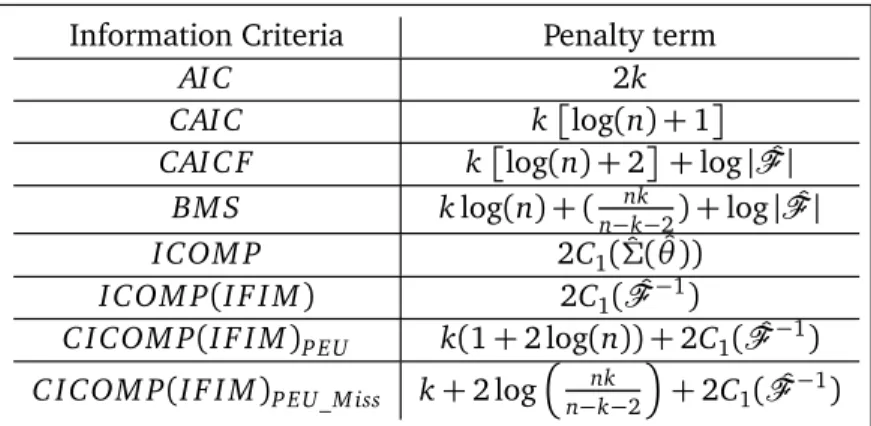
ComparingAI C,CAI C,CAI C F,BM S, and the different forms ofI COM P-type criteria, we see that the difference between these criteria are in their penalty terms. For convenience, we summarize these model selection criteria in Table 1, which we will use in our numerical ex-amples. In the next section we give two numerical examples to demonstrate the performance
Table1: SummaryofInformationCriteriaandTheirPenalties.
Information Criteria Penalty term
AI C 2k
CAI C klog(n) +1
CAI C F klog(n) +2+log|F |ˆ
BM S klog(n) + (n−nkk−2) +log|F |ˆ
I COM P 2C1( ˆΣ( ˆθ))
I COM P(I F I M) 2C1( ˆF−1)
C I COM P(I F I M)P E U k(1+2 log(n)) +2C1( ˆF−1) C I COM P(I F I M)P E U_M iss k+2 logn−nkk−2+2C1( ˆF−1)
of these information criteria in SEM.
5. Numerical Results
5.1. A Large Scale Monte Carlo Simulation Study
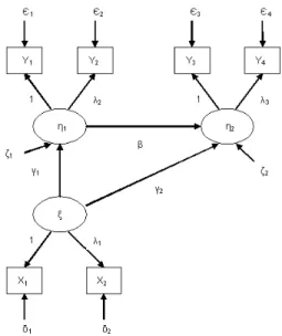
In this simulation study, we used the widely known general SEM simulation protocol given in [15]. This model is formed from 1 latent exogenous variable, 2 latent endogenous vari-ables, 2 observed exogenous varivari-ables, and 4 observed endogenous variables. We slightly modify the structure of [15] in θε matrix to achieve convergence in LISREL. We generated
500 sample covariance matrices for four sample sizes (100, 400, 1000, and 4000). Each sam-ple covariance matrix was analyzed for each of the three analytic models given below using LISREL.
Figure 1 shows the population parameters of the model and the path diagram as expressed in LISREL notation, with parameters shown here.
Λx =
1.00 0.50
,Λy =
1.00 0 0.95 0 0 1.00 0 0.90
,Γ =
−0.60
−0.25
,Φ =7,B=
0 0 0.60 0 , Ψ = 5.00 0 0 4.00
,θδ=
3.00 0 0 2.50
,θε=
3.00 0 0 0
0 3.00 0 0
0 0 4.00 0
0 0 0 4.00
Once the model parameters are specified, the implied population covariance matrix is
ob-Figure1: Truemodelwithpopulationparametersandmodelspeiationonditions.
tained through Equation (5). For the analysis of this covariance matrix, we used three differ-ent analytic models, given below.
• Overfitting model: AM1 (15 free parameters)
Λx(1, 1) = Λy(1, 1) = Λx(3, 2) =1
Γ,Φ,B,Ψ,θδ,θεare estimated freely
Λx =
1.00
λ1
,Λy =
1.00 0
λ2 0
0 1.00
0 λ3
,Γ =
γ1
γ2
,Φ =φ,B=
0 0 β 0 , Ψ =
ψ1 0 0 ψ2
,Θδ=
θδ1 0
0 θδ2
,Θε=
θε1 0 0 0
0 θε2 0 0
0 0 θε3 0
0 0 0 θε4
• Pseudo true model: AM2 (13 free parameters)
Λx(1, 1) = Λy(1, 1) = Λx(3, 2) =1
θε(1, 1) =θε(2, 2),θε(3, 3) =θε(4, 4) Γ,Φ,B,Ψ,θδ are estimated freely
Λx =
1.00
λ1
,Λy =
1.00 0
λ2 0
0 1.00
0 λ3
,Γ =
γ1
γ2
,Φ =φ,B=
0 0
β 0
Ψ =
ψ1 0 0 ψ2
,Θδ=
θδ1 0
0 θδ2
,Θε=
θε1 0 0 0
0 θε1 0 0
0 0 θε3 0
0 0 0 θε3
• Underfitting model: AM3 (11 free parameters)
Λx(1, 1) = Λy(1, 1) = Λx(3, 2) =1
Λx(2, 1) = Λy(2, 1) Γ(2, 1) =0
θε(1, 1) =θε(2, 2),θε(3, 3) =θε(4, 4) Φ,B,Ψ,θδ are estimated freely
Λx =
1.00
λ1
,Λy =
1.00 0
λ1 0
0 1.00
0 λ3
,Γ =
γ1 0
,Φ =φ,B=
0 0 β 0 , Ψ =
ψ1 0 0 ψ2
,Θδ=
θδ1 0
0 θδ2
,Θε=
θε1 0 0 0
0 θε1 0 0
0 0 θε3 0
0 0 0 θε3
Based on the above AM structures above, we carried out a large scale Monte Carlo simulation study. Since we have three AMs and four different sample sizesn=100, 400, 1000, and 4000, we have in total 12 different simulation experiments. For each simulation experiment, we performed 500 replications and scored each of the information criteria to study their empirical performance based on their hit ratios.
One of the important characteristics of AM3 is that it is a misspecified model according to[15]; that is misspecified as it relates to underfitting . We note that his misspecification does not indicate to distributional misspecification since there are many other ways we can misspecify a model.
The steps of our Monte Carlo simulation are as follows,
1. The covariance matrices are generated with population parameters given in Figure 1, using PRELIS.
2. Each generated sample covariance matrix is analyzed by means of the three analytic models using LISREL. Goodness of fit indices and implied covariance matrices from LISREL outputs are saved.
3. LISREL outputs are passed to program are read into MATLAB, which computes both
5.1.1. Results of Monte Carlo Simulation Experiments
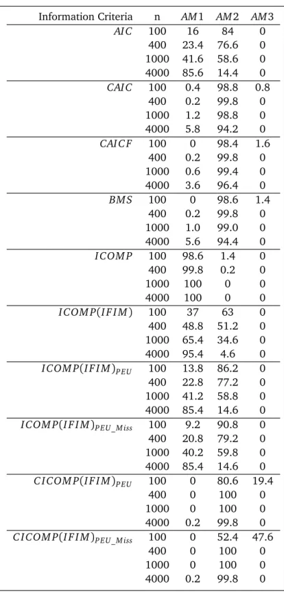
Table2: Corretmodelseletionfrequeny byriteria(in%).
Information Criteria n AM1 AM2 AM3
AI C 100 16 84 0
400 23.4 76.6 0
1000 41.6 58.6 0
4000 85.6 14.4 0
CAI C 100 0.4 98.8 0.8
400 0.2 99.8 0
1000 1.2 98.8 0
4000 5.8 94.2 0
CAI C F 100 0 98.4 1.6
400 0.2 99.8 0
1000 0.6 99.4 0
4000 3.6 96.4 0
BM S 100 0 98.6 1.4
400 0.2 99.8 0
1000 1.0 99.0 0
4000 5.6 94.4 0
I COM P 100 98.6 1.4 0
400 99.8 0.2 0
1000 100 0 0
4000 100 0 0
I COM P(I F I M) 100 37 63 0
400 48.8 51.2 0
1000 65.4 34.6 0
4000 95.4 4.6 0
I COM P(I F I M)P E U 100 13.8 86.2 0
400 22.8 77.2 0
1000 41.2 58.8 0
4000 85.4 14.6 0
I COM P(I F I M)P E U_M iss 100 9.2 90.8 0
400 20.8 79.2 0
1000 40.2 59.8 0
4000 85.4 14.6 0
C I COM P(I F I M)P E U 100 0 80.6 19.4
400 0 100 0
1000 0 100 0
4000 0.2 99.8 0
C I COM P(I F I M)P E U_M iss 100 0 52.4 47.6
400 0 100 0
1000 0 100 0
In our simulation study, we intentionally did not include the nine traditional goodness of fit indices which were scored in[15], as they do not have the provision of taking into account different type of model misspecifications. Therefore, it is misleading even to score and report their results under such circumstances.
In Table 2, we summarize our result of percent hit ratios of the three AMs, AI C CAI C,
CAI C F, BM S, I COM P, I COM P(I F I M), I COM P(I F I M)P E U,I COM P(I F I M)P E U_M iss,
C I COM P(I F I M)P E U, and C I COM P(I F I M)P E U_M iss criteria, for each sample size. We note thatCAI C,CAI C F, BM S, I COM P, I COM P(I F I M), I COM P(I F I M)P E U,
I COM P(I F I M)P E U_M iss,C I COM P(I F I M)P E U, andC I COM P(I F I M)P E U_M issall hit the pseudo trueAM2 with very high frequencies. Specifically the performances ofCAI C, CAI C F, BM S,
C I COM P(I F I M)P E U, andC I COM P(I F I M)P E U_M issare outstanding and all above 90%. We further observe thatAI C’s performance is not satisfactory as the sample size increases. For sample sizes n = 100, AI C picks AM2 84% of the time, and as n gets large, AI C’s hit percentage diminishes, and deteriorates. We know that AI C is not a consistent criterion. Specifically,AI C leans toward the AM1 which is an overfitting model which is the behaviour that is often demonstrated in the literature aboutAI C.
Of course one should note that, the large scale Monte Carlo simulation experiment we performed is only using one model set here. This can be easily extended to a large dimensional other model settings to further study the performances of these criteria in SEM. This requires high speed computation and computational capability on a super computer and a stand alone SEM software to carry out the task that is limited at this point.
5.2. A Real Data Example in Market Research
In this example, we apply the information criteria to a real data set from a soft drink company in Turkey. For propriety reasons we cannot disclose the name of the company. The data set in this study consists of a sample ofn=135 marketing surveys to study the product quality and to build a predictive operating model for the soft drink company. The goal of this survey was to enhance the market positioning and determine the influence of the investment of the company on their marketing campaign. For this data set we have seven characteristics which are measured to establish the companies objectives. These seven characteristics are:
refreshing,tastes great, good with meal, exhilarating,feels good,worth the money, andbrands having products of good quality.
Since we do not know a priori the generating model for this real data set, first we applied an Exploratory Factor Analysis (EFA) to learn which factors were related to the original vari-ables. According to EFA results, three latent variables were named as“taste”, “feeling”, and
“quality”, based on pre-determined factors. In the EFA model, variables which were loaded with factor 1 were: “refreshing”, “tastes great”, and “good with meal”. These were taken as exogenous variables and related to the latent exogenous variable“taste”.
Figure2: FullSEMwith17freeparameters(Model1).
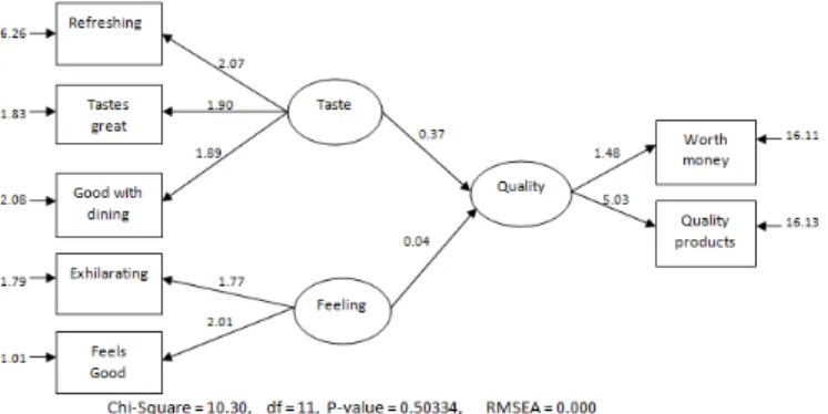
Figure3: FullSEMwith15freeparameters(Model2).
Since the information criteria used in the study were not applied to the just identified models, over-identified models were chosen. In accordance with the t-rule[19], one of the rules of identification must have free parameters under 28 to be over identified. Accordingly, three different models with free parameters, 17, 15, and 13 were compared to assess the information criteria. The path diagram of each of these three models, obtained from LISREL, are given in Figures 2, 3, and 4. Model 1 was fit to the data with 17 free parameters in Figure 2 withP−value=0.29>0.05. In this model, the diagonal elements of the covariance of latent exogenous variables and a single path coefficient between latent and observed endogenous were fixed. The other parameters were estimated freely. Model 2 was fit to the data with 15 free parameters shown in Figure 3 with P−value=0.42>0.05. It was restricted by setting to 1 a single path coefficient in each latent variable, and equating diagonal elements of the covariance matrix of latent variables. In the case of Model 3, the model was fit to the data with 13 free parameters shown in Figure 4 with P−value = 0.00009< 0.05. It also was restricted by setting to 1 as single path coefficient in each latent variable, and equating the measurement errors of the observed variables belonging to each latent variable.
All information criteria scores for each of these three SEMs, obtained from LISREL and our MATLAB module, are reported in Table 3. According to the minimum of the information
Table3: ThevaluesofriteriaforthreeGeneralSEMs.
Model Selection Criteria Model 1 Model 2 Model 3
AI C 4218.1 4216.6 4298.8
CAI C 4284.5 4275.2 4349.5
CAI C F 4333.8 4322.4 4389.0
BM S 4319.6 4309.5 4377.6
I COM P 4187.9 4190.5 4275.9
I COM P(I F I M) 4245.7 4248.6 4328.3
I COM P(I F I M)P E U 4279.7 4278.6 4354.3
I COM P(I F I M)P E U_M iss 4285.2 4282.9 4357.5
C I COM P(I F I M)P E U 4429.4 4410.8 4468.8
C I COM P(I F I M)P E U_M iss 4456.8 4432.0 4484.8
criteria, we choose the “best” model among those compared, as the model that achieves the best balance of fit with respect to parameter cardinality. In this case, all criteria are minimized at Model 2. These are indicated by the boldfaced scores in Table 3. We note that for this data set all criteria agreed. In general, this would not typically be the case with other real data sets.
6. Conclusions and Discussion
In this paper, we showed the performance of several information criteria, some old and new ones in general SEMs, under different sample sizes, and different models. Based on our results from this specific large scale Monte Carlo simulation experiment, for general SEM,
CAI C, CAI C F, BM S, C I COM P(I F I M)P E U and C I COM P(I F I M)P E U_M iss criteria show the best performance. On the other hand, the performance of AI C seems to degrade as sample sizes increase - it tends to select overfitting models. This behavior is based on the sensitivity of the log likelihood function to sample size. BecauseCAI C,CAI C F,BM S,C I COM P(I F I M)P E U
and C I COM P(I F I M)P E U_M iss criteria are consistent with respect to sample size (penalty term includes log(n)), they become more accurate as the sample size gets larger. Our sim-ulation results demonstrates the performance and the versatility of these criteria. In sum-mary, we recommend that the information criteria: CAI C F, BM S, C I COM P(I F I M)P E U and
C I COM P(I F I M)P E U_M iss, be used in SEM. In the real example, we showed how one can build an operating predictive SEM in market research. We are currently studying other forms of misspecification such as the distributional misspecification, presence of high multicollinear-ity, and error variance heteroscedasticity within the SEM framework using the information criteria along with other applications. Our results will be reported elsewhere.
ACKNOWLEDGEMENTS This research was supported by the Scientific and Technological Research Council of Turkey (TUBITAK) for the first author at the Department of Statistics, Operations, and Management Science at the University of Tennessee as a Visiting Scholar under the supervision of Professor Bozdogan. The first author extends her gratitude and thanks to Professor Bozdogan for the hospitality and conducive research atmosphere provided.
References
[1] H Akaike. Information theory and an extension of the maximum likelihood principle. In B.N. Petrox and F. Csaki, editors, Second International Symposium on Information Theory., pages 267–281, Budapest, 1973. Academiai Kiado.
[2] H Akaike. Factor analysis and AIC. Psychometrica, 52(3):317–332, 1987.
[3] K A Bollen. Structural Equations with Latent Variables. John Wiley,New York, 1989.
[4] H Bozdogan. Model selection and akaike’s information criteria (AIC): the general theory and its analytical extensions. Psychometrica, 52:317–332, 1987.
[5] H Bozdogan. A new information theoretic measure of complexity index for model eval-uation in general structural eqeval-uation models with latent variables. Rutgers the State Univarsity, June 13-16 1991. Symposium on Model Selection in Covariance Structures at the Joint Meeting of Psychometric Society and The Classification Society.
Approaches in Classification and Data Analysis, pages 169–177. Springer-Verlag, New York, 1994.
[7] H Bozdogan. Akaike’s information criterion and recent developments in information complexity. Journal of Mathematical Psychology, 44:62–91, 2000.
[8] H Bozdogan. Statistical Data Mining Knowledge Discovery, chapter Intelligent Statisti-cal Data Mining with Information Complexity and Genetic Algorithms., pages 15–56. ChapmanHall,CRC, 2004.
[9] H Bozdogan. A new class of information complexity (ICOMP) criteria with an applica-tion to customer profiling and segmentaapplica-tion. Journal of the School of Business Adminis-tration, 39(2):370–398, 2010.
[10] H Bozdogan and M Ueno. A unified approach to information-theoretic and bayesian model selection criteria. Crete, Greece, 2000. The 6th World Meeting of the Interna-tional Society for Bayesian Analysis.
[11] N Cliff. Some cautions concerning the application of causal modeling methods. Multi-variate Behavioral Research, 18:115–126, 1983.
[12] H Cramér. Mathematical Methods of Statistics. Princeton University Press, Princeton, New Jersey, 1946.
[13] E Deniz, H Bozdogan, and S Katraggadda. Structural equation modeling (SEM) of cate-gorical and mixed-data using the novel gifi transformations and information complexity (ICOMP) criterion.Journal of the School of Business Administration, 40(1):86–123, 2011.
[14] E A Deniz. Information Criteria in Structural Equation Models.unpublished ph.d. thesis, Mimar Sinan Fine Arts University, 2007.
[15] X Fan and X Fan. Using SAS for monte carlo simulation research in SEM. Structural Equation Modeling, 12(2):299–333, 2005.
[16] B Frieden.Physics from Fisher Information.Cambridge University Press, Cambridge, UK, 1998.
[17] N Gheissari and A Bab-Hadiashar. Detecting cylinders in 3D range data using model selection criteria. Proceeding of Fifth International Conference on 3-D Digital Imaging and Modelling, 2005.
[18] K Jöreskog. Testing Structural Equation Models., chapter Testing Structural Equation Models. Sage Publication, London, 1993.
[19] K Jöreskog and D Sörbom.LISREL 7 A Guide to the Program and Applications 2nd Edition.
[20] S Kullback. Information Theory and Statistics. Dover Publications, Dover, New York, 1968.
[21] S Kullback and R Leibler. On information and sufficiency. Annals of Mathematical Statis-tics, 22:79–86, 1951.
[22] S A Mulaik.Linear Causal Modeling with Structural Equations.Chapman and Hall, 2009.
[23] C R Rao. Information and accuracy attainable in the estimation of statistical parameters.
Bulletin of the Calcutta Mathematical Society, 37:81, 1945.
[24] C R Rao. Minimum variance and the estimation of several parameters. InProceedings of the Cambridge Philosophical Society., volume 43, page 280, 1947.
[25] C R Rao. Sufficient statistics and minimum variance estimates. In Proceedings of the Cambridge Philosophical Society., volume 45, page 213, 1948.
[26] J Rissanen. Modeling by shortest data description. Automatica, pages 465–471, 1978.
[27] Y Sakamoto, M Ishiguro, and G Kitagawa. Akaike Information Criterion Statistics. Dor-drecht, The Netherlands: Reidel, 1986.
[28] G Schwarz. Estimating the dimension of a model. Annals of Statistics, pages 461–464, 1978.
[29] M Van Emden. An analysis of complexity. InMathematical Centre Tracts., volume 35. Mathematisch Centrum, 1971.