An Intelligent System for Classification of the Communication
Formats Using PSO
Ata E. Zadeh Shermeh and Reza Ghaderi Faculty of Electrical and Computer Engineering, Babol Noushirvani University of Technology, Iran E-mail: [email protected], [email protected]
Keywords: classification of communication signals, particle swarm, higher order statistics, supervised learning
Received: May 23, 2007
Text Automatic identification of digital signal types is of interest for both civil and military applications. This paper presents an efficient signal type identifier that includes a variety of digital signals. In this method, a combination of higher order moments (HOM) and higher order cumulants (HOC) are used as the features. A multi-layer perceptron neural network with SASS learning algorithm is proposed to determine the membership of the received signal. We have used swarm intelligence (SI) for feature selection in order to reduce the complexity of the classifier. Simulations results show that the proposed
method has high performance for identification of different kinds of digital signal even at very low
SNRs. This high efficiency is achieved with only seven features, which have been selected using particle swarm optimizer.
Povzetek: Opisana je metoda za identifikacijo digitalnih signalov.
1
Introduction
Automatic signals type recognition is an important topic for both the civil and military domain. Signal type recognition classification is also believed to play an important part in future 4G software radios [1]. The general idea behind the software radio architecture is to perform a considerable amount of the signal processing in software instead of it being defined in hardware. This would enable the radio to adapt to a changing environment and user requirements by simply updating the software or by using adaptable software systems. In such scenarios, a broadcaster could for example change to appropriate modulation schemes according to the capacity of the channel. A receiver incorporating automatic modulation recognition could then handle this in real times.
Automatic signal classification methods, usually, divided two principle techniques. One is the decision theoretic approach and the other is pattern recognition. Decision theoretic approaches use probabilistic and hypothesis testing arguments to formulate the recognition problem [2-3]. These methods suffer from their very high computational complexity, difficulty to implementation and lack of robustness to model mismatch [7]. Pattern recognition approaches, however, do not need such careful treatment. They are easy to implement. They can be further divided into two subsystems: the feature extraction subsystem and the classifier subsystem. The former extracts prominent characteristics from the raw data, which are called features, and the latter is a classifier [4-14].
In [9], for the first time, Ghani and Lamontagne proposed using the multi-layer perceptron (MLP) neural
cyclic spectrum posses more advantage than power spectrum in signal type recognition. A full-connected backpropagation neural network is used for classification in that research. The success rate of this identifier is reported around 90% with SNR ranges 5-25 dB.In [14], the authors have used a combination of the symmetry, fourth order cumulants and power moments of the received signals as the features for identification of PSK2, PSK4, PSK8, QAM16 and QAM32. The classifier was a modified MLP neural network (with few output nodes). They reported a success rate about 92% at SNR of 8dB. In [15], the authors have introduced an identifier based on discrete wavelet decompositions and adaptive network based fuzzy interference system for recognition of ASK8, FSK8, PSK8 and QASK8.
Most of the methods can only recognize a few types of digital signal and/or lower order of digital signal types. They usually need high SNRs in order to achieve the minimum acceptable performance (80%). Basically, this is due to the classifier and the features that are used. Finding the suitable features is a very important step for recognition of these digital signals. From the published works it can be found that the methods, which use the higher order statistical features, are able to include the digital signal types such as QAM and higher orders of digital signals [6-12]. In this paper we have used a combination of the higher order moments and higher order cumulants (up to eighth) as the effective features for recognition of the considered digital signals. The identifiers that use artificial neural networks (ANNs) as the classifier have high performances [12-14]. In this paper we have used a multi-layer perceptron (MLP) neural network with self adaptive step-size (SASS) learning algorithm as the classifier [15]. We have used particle swarm optimization, in order to reduce the complexity of the proposed identifier.
The paper is organizes as follows. Section 2 describes the feature extraction module. Section 3 presents the classifier. Optimization module is introduced in Section 4. Section 5 shows some simulation results. Finally, Section 6 concludes the paper.
2
Feature extraction
A typical pattern recognition system after doing some pre-processing operations, often reduce the size of a raw data set by extracting some distinct attributes called features. The need for feature extraction comes to scene due to the possible inability to use the raw data. These features define a particular pattern. In the signal recognition area, choosing the good features, not only enable the classifier to distinguish more and higher digital signals, but also help to reduce the complexity of the classifier.
In this paper we have considered the following digital signals: ASK2, ASK4, ASK8, PSK2, PSK4, PSK8, QAM16, QAM32, QAM64, Star-QAM8, and V32. For simplifying the indication, the signals ASK2, ASK4, ASK8, PSK2, PSK4, PSK8, QAM16, QAM32, QAM64, Star-QAM8, and V32 are substituted with P1, P2, P3, P4,
P5, P6, P7, P8, P9, P10, and P11 respectively. Different
types of the digital signal have different properties; therefore finding the proper features in order to identify them (especially in case of higher order and/or non-square) is a difficult task. Based on our researches, a combination of the higher order moments and higher order cumulants up to eighth make provide a fine way for discrimination of the considered digital signal types.
Probability distribution moments are a generalization of concept of the expected value, and can be used to define the characteristics of a probability density function [16]. The auto-moment of the random variable may be defined as follows:
] ) ( [ pq q pq E s s
M = − ∗ (1) where pcalled moment order and s∗ stands for complex
conjugation. Now, consider a zero-mean discrete based-band signal sequence of the formsk =ak + jbk. Using the definition of the auto-moment, the expressions for different order may be easily derived.
Consider a scalar zero mean random variables. The symbolism for pthorder of cumulant is:
] ,..., , ,..., [
) ( )
(p12q3terms 142qterms43 pq Cum s s s s
C ∗ ∗
−
= (2)
3
Classifier
We have used a MLP neural network as the classifier. A MLP neural network consists of an input layer of source nodes, one or more hidden layers of computation nodes (neurons) and an output layer [17]. The number of nodes in the input and the output layers depend on the number of input and output variables, respectively. In this paper a single hidden layer MLP neural network was chosen as the classifier. The issue of learning algorithm is very important for MLP. Backpropagation (BP) learning algorithm is still one of the most popular algorithms. In BP a simple gradient descent algorithm updates the weight values. However under certain conditions, the BP network classifier can produce non-robust results and easily converge to local minimum. Moreover it is time consuming in training phase. New algorithms have been proposed so far in order to network training. However, some algorithms require much computing power to achieve good training, especially when dealing with a large training set.
In this paper, SASS learning algorithm is used [17]. SASS is an adaptive step-size method. it is based on the bisection method for minimization in one dimension, in which the minimum of a valley is found by taking a step in the descent direction of half the previous step. The method has been adapted to allow the step-size to both increase and decrease. It uses the same update rule resilient but updates ∆ij differently. It uses two previous
⎪ ⎪ ⎪ ⎪ ⎩ ⎪⎪ ⎪ ⎪ ⎨ ⎧ − ∆ ≥ Ε − Ε ≥ Ε − Ε − ∆ = ∆ otherwise t t w t w and t w t w if t ij ij ij ij ij ij t ij ); 1 ( * 5 . 0 0 ) ( ) 2 ( 0 ) ( ) 1 ( ); 1 ( * 0 . 2 ) ( δ δ δ δ δ δ δ δ (3)
This update value adaptation process is then followed by the actual weight update process, which is governed by the following equation:
) ( ) ( ) 1
(t w t w t
wij + = ij +∆ ij (4)
4
Swarm intelligence
There were a large number of features involved in the study as it was found in Section 2. Although some of these features may carry good classification information when treated separately, there is little gain if they are combined together (due to sharing the same information content). The easiest way to reduce the number of features is feature selection. The advantage of feature selection is that one can use the least possible number of features without compromising the performance of the identifier. In this paper we use the particle swarm optimization (PSO) for feature subset selection.
The particle swarm optimization (PSO) algorithm was first introduced in 1995 [18]. The basic operational principle of the particle swarm is reminiscent of the behavior of a group of a flock of birds or school of fishes or the social behavior of a group of people. Each individual is considered as a volume-less particle (a point) in the N-dimensional search space. The index of the best particle among all the particles in the population (global model) is represented by the symbol g. The index of the best particle among all the particles in a defined topological neighborhood (local model) is represented by the index subscript l. The particle variables are manipulated according to the following equation (global model [18]): )) 1 ( ( * () 2 * )) 1 ( ( * () 1 * ) 1 ( * ) ( 2 1 − − + − − + − = t x p rand c t x p rand c t v w t v in gn in in in i in (9) ) ( ) 1 ( )
(t x t v t
xin = in − + in (10) where n is the dimension (1≤n≤N) , c1and c2 are positives constants, rand1()and rand2() are two random functions in the range [0,1], and w is the inertia weight. Xi(t)=(xi1(t),xi2(t),...,xiN(t))presents the the ith particle at time step t. Pi(t)=(pi1,pi2,...,piN)records the best previous position (the position giving the best fitness value) of the ith particle. () ( (), (),... ())
2
1 t v t v t v
t
Vi = i i iN
presents the rate of the position (velocity) for particle i at the time step t.
The constants c1and c2 in above equation represent the weighting of the stochastic acceleration terms that pull each particle toward pbest and gbest positions. Thus,
adjustment of these constants changes the amount of ‘tension’ in the system. Low values allow particles to roam far from target regions before tugged back, while high values result in abrupt movement toward, or past, target regions. The inertia weight w controls the impact of the previous histories of velocities on the current velocity, thus influencing the trade-off between global (wide-ranging) and local (nearby) exploration abilities of the ‘flying points’. By linearly decreasing the inertia weight from a relatively large value to a small value through the course of the PSO run (total number of generations prior termination), the PSO tends to have more global search ability at the beginning of the run while having more local search ability near the end of the run [19].
5
Simulation results
This section presents the some simulation results of the proposed identifier. All signals are digitally simulated in MATLAB editor. We assumed that carrier frequencies were estimated correctly (or to be known). Thus, we only considered complex base-band signals. Gaussian noise was added according to SNRs, –5, 0, 5, 10, and 15dB to the simulated signals. Each signal type has 2400 realizations. These are then divided into training, validation and testing data sets. The activation functions of tan-sigmoid and logistic were used in the hidden and the output layers, respectively. The MSE is taken to be10-6. The MLP classifier is allowed to run up to 5000 training epochs. Based on our extensive experiments it seems that the number of 20 neurons is adequate for reasonable identification.
5.1
Performance of identifier without
feature selection
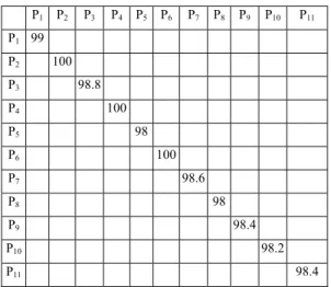
In this subsection, we evaluate the performance of straight proposed identifier (SPROI), i.e. full features are used. Tables 1-2 show the correct matrix of identifier at two selected values of SNR. Table 3 shows the performances of the identifier at various SNRs. It can be seen that the performances of identifier is generally very good at low SNRs. Also, we have evaluated the performance of the identifier at a high SNR value. Table 4 indicates the training performance of identifier at SNR= 50dB. The classifier can show up to 100% success rate.
Table3: Correct matrix of the identifier (without feature selection) at SNR=5dB.
P1 P2 P3 P4 P5 P6 P7 P8 P9 P10 P11
P1 97.2
P2 97.8
P3 96.6
P4 100
P5 96
P6 97
P7 93.4
P8 97
P9 94.5
P10 98
Table2: Correct matrix of the identifier (without feature selection) at SNR=10dB.
P1 P2 P3 P4 P5 P6 P7 P8 P9 P10 P11
P1 99
P2 100
P3 98.8
P4 100
P5 98
P6 100
P7 98.6
P8 98
P9 98.4
P10 98.2
P11 98.4
Table3: The performances of the identifier (without feature selection) at different SNR values.
SNR Training Testing
-5 85.45 83.76
0 89.85 88.52
5 96.75 96.55
10 98.90 98.85 15 99.25 99.14
Table4: The performances of identifier (without feature selection) at SNR=50dB.
P1 P2 P3 P4 P5 P6 P7 P8 P9 P10 P11
P1 100
P2 100
P3 100
P4 99.6
P5 100
P6 100
P7 100
P8 99.6
P9 100
P10 99.8
P11 99.4
As mentioned the speed of learning algorithm is an important issue for MLP. The efficiency of the learning algorithm affects the amount of experimentation that can be done. To indicate the effectiveness of chosen learning algorithm (SASS), we have compared it with the SUPERSAB learning algorithm that is an adaptive learning rate algorithm [20]. In SUPERSAB learning algorithm each weightwij, connecting node j with node i, has its own learning rate that can vary in response to error surface. The system that uses MLP with SUPERSAB learning algorithm as the classifier is named as TECH2. Based our experiments, any number in the vicinity of 40 neurons seems to be adequate for reasonable classification. Other simulations setup is the
same. Table 5 shows the performance of TECH2. Table 8 presents the comparison between SPROI (that uses MLP with SASS learning algorithm as the classifier) and TECH2. It can be seen that the performance of the SPROI (that uses MLP with SUPERSAB learning algorithm as the classifier). It can bee seen that SPRRO has better performance than TECH2.
Table7: The performance of TECH2 at different levels of SNR.
SNR Training Testing
-5 73.46 72.35
0 82.42 80.24
5 86.70 85.42
10 94.64 92.45
15 96.25 94.65
Table6: Comparison between SPROI and TECH2: the testing performance and the number of epochs that are needed.
SASS SUPERSAB
SNR Passed
Epochs Testing
Passed
Epochs Testing
-5 725 83.76 1245 72.35
0 324 88.52 685 80.24
5 565 96.55 1575 85.42
10 364 98.85 978 92.45
15 485 99.14 1245 94.65
5.2
Performance of the identifier with
using the optimizer
We have tested the identifier using several features selected using PSO. The selection of the PSO parameters plays an important role in the optimization.
Table 7 shows the performances of the identifier using four features selected by PSO. Table 8 shows this performance using seven features selected by PSO. Table 9 show the performance of the identifier using eighteen features selected by PSO. Also in these tables the performances of identifier without feature selection is showed. It can be seen that in Table 8 the identifier records a performance degradation less than 1% only at SNR= -5dB. For other levels of SNR, the difference is negligible. Thus it can be said that the proposed method achieves high performance on most SNR values with only seven features that have been selected using PSO. Tables 10-11 show the correct matrices of identifier at SNR= 5 dB and SNR=10 with seven features that have been selected by PSO. It is found that proposed is able to identify the different types of digital signal with high accuracy only seven selected features using PSO.
Table7: Testing performance (TP) of the identifier with five features selected using PSO.
SNR TP with applying PSO TP without PSO
-5 80.15 83.76
0 83.25 88.85
5 91.20 96.55
10 94.68 98.85
Table8: Testing performance (TP) of the identifier with seven features selected using PSO.
SNR TP with applying PSO TP without PSO
-5 82.90 83.76
0 88.25 88.85
5 96.18 96.55
10 98.50 98.85
15 99.02 99.14
Table9: Testing performance (TP) of the identifier with twenty features selected using PSO.
SNR TP with applying PSO TP without PSO
-5 83.45 83.76
0 88.60 88.85
5 96.25 96.55
10 98.65 98.85
15 99.08 99.14
Table12: Correct matrix of PROI with only seven features selected using PSO at SNR=5dB.
P1 P2 P3 P4 P5 P6 P7 P8 P9 P10 P11
P1 97
P2 97
P3 96.5
P4 100
P5 95
P6 97
P7 92.5
P8 97
P9 94
P10 97.5
P11 94.5
Table13: Correct matrix of PROI with only seven features selected using PSO at SNR=10dB.
P1 P2 P3 P4 P5 P6 P7 P8 P9 P10 P11
P1 99
P2 100
P3 99
P4 100
P5 97
P6 100
P7 98
P8 98
P9 97.5
P10 97
P11 98
As mentioned the features play a vital role in signal identification. In order to indicate the effectiveness of the chosen features, we have used the features that have been introduced in [7]. We name this identifier as THECH3. Other simulations setup is the same. Figure1 show a
comparison between TECH3 and our proposed identifier (PROI) at different SNRs. Results imply that our chosen features have effective properties in signal representation.
Figure1: Performances comparison between PROI and TECH3.
6
Conclusions
features set for identification the different types of digital signal.
References
[1] K.E. Nolan, L. Doyle, P. Mackenzie, D. O. Mahony (2002). Modulation Scheme Classification for 4G Software Radio Wireless Network. Proc. IASTED. [2] W. Wei and J. M. Mendel, “Maximum-likelihood
classification for digital amplitude-phase modulations,” IEEE Trans. Commun.,vol. 48, pp. 189-193, 2000.
[3] P. Panagotiou, and A. Polydoros, “Likelihood ratio tests for modulation classifications,” Proc. MILCOM, pp. 670-674, 2000.
[4] S. Z. Hsue, and S. S. Soliman, Automatic modulation classification using Zero-Crossing, IEE Proc. Radar, Sonar and Navigation, vol. 137, 1990, pp. 459-464.
[5] B. G. Mobasseri, “Digital modulation classification using constellation shape,” Signal Processing, vol. 80, pp. 251–277, 2000.
[6] J. Lopatka, and P. Macrej, “Automatic modulation classification using statistical moments and a fuzzy classifier,” Proc. ICSP, pp.121-127, 2000.
[7] A. Swami, and B. M. Sadler, “Hierarchical digital modulation classification using cumulants,” IEEE Trans. Comm., vol. 48, pp. 416–429, 2000.
[8] C. M. Spooner, “Classification of cochannel communication signals using cyclic cumulants,” Proc. ASILOMAR, pp. 531-536, 1995.
[9] O. A. Dobre, Y. Bar-Ness, and W. Su, “Robust QAM modulation classification algorithm based on cyclic cumulants,” Proc WCNC, pp. 745-748, 2004. [10] A. E.Shermeh, D. Movahedi, “Signal identification
using an efficient method,” ICS 2007.
[11] C. M. Spooner, W. A. Brown, and G. K. Yeung, “Automatic radio-frequency environment analysis,” Proc. ASILOMAR, pp. 1181-1186, 2000.
[12] A. E. Shermeh, D. Movahedi, “Automatic digital modulation identification using an intelligent method,” ICS 2007.
[13] C. L. P. Sehier, “Automatic modulation recognition with a hierarchical neural network,” Proc. MILCOM, pp. 111–115, 1993.
[14] A.K. Nandi, E.E. Azzouz, “Algorithms for automatic modulation recognition of communication signals,” IEEE Trans. Comm., vol. 46, pp. 431–436, 1998.
[15] E. Avci, D. Hanbay and A. Varol, “An expert disceret wavelet adaptive network based fuzzy inference system for digital modulation recognition,” Expert Systems with Applications, 2006.
[16] J. Hannan, M. bishop, “ A class of fast artificial NN learning algorithms”, Tech. Report, JMH-JMB 0/96, Dep. of Cybernetics, University of Reading, 1996.
[17] C. L Nikias and A. P. Petropulu, Higher-Order Spectra Analysis: A Nonlinear Signal Processing
Framework. Englewood Cliffs, NJ: PTR Prentice-Hall,1993.
[18] S. Haykin, Neural Networks: A Comprehensive Foundation. New York: MacMillan, 1994.
[19] R. C. Eberhart, and J. Kennedy, A new optimizer using particle swarm theory, Proc. ISMMH S, 1995, pp. 39-43.
[20] Y. Shi and R. C. Eberhart, A Modified Particle Swarm Optimizer, in Proc. IJCNN, 1999, pp. 69-73.