EVIDENCE ON BAC 08 LAWS
DONALD G. FREEMAN*
This article reexamines the effectiveness of blood alcohol content (BAC) laws in reducing traffic fatalities. Differences-in-differences estimators of U.S. state-level data with standard errors corrected for autocorrelation show no evidence that low-ering the BAC limits to 0.08 g/dL reduced fatality rates, either in total or in crashes likely to be alcohol related, or in states that passed BAC 08 in laws either in advance of or in response to federal pressure. Other legislations, including administrative license revocation and primary seat belt laws, are found effective in reducing fatalities in all specifications. Endogeneity tests using event analyses confirm the
differences-in-dif-ferences estimates.(JEL I18, K32)
I. INTRODUCTION
The past 25 yr have witnessed a sea change in attitudes and legislation regarding driving under the influence (DUI) of drugs and alco-hol. Although the first laws against drunk driving were passed as long ago as 1910 by New York and by California in 1911, statutes in most states prior to about 1980 simply pro-hibited ‘‘driving while intoxicated,’’ without providing specific guidelines to define ‘‘intoxi-cated.’’ As a result, much discretion was involved in the arrest and prosecution of drinking drivers, and punishment was often light, even for chronic offenders.
In the early 1980s, however, under pressure from insurance companies and advocacy groups such as Mothers Against Drunk Driv-ing (MADD) and accompanied by threats of loss of federal highway funds for noncompli-ance, all states passed tougher drunk driving statutes, often incorporating explicit measures of presumed alcohol impairment. In 1980, for example, only 15 states had legislation estab-lishing a permissible blood alcohol content (BAC), with 0.10 g/dL then defined as the pre-sumed level of intoxication. By 2005, after
a renewed push again involving pressure from highway funding, all states had a BAC limit at a lower threshold of 0.08 g/dL.
BAC laws have been accompanied by a raft of other alcohol-control measures: MADD (2005) lists 39 pieces of recommended state legislation for the prevention of drunk driving, ranging from administrative license revoca-tion (ALR)1to zero tolerance (ZT) of drinking by minor drivers; by 2005, the median state had passed 27 pieces, and all had passed at least 17.
Clearly, progress has been made in getting drunk drivers off the streets. Advances in automotive safety engineering over time have led to declines in fatalities from all causes, but from 1982, the first year for which reliable measures of victims’ BAC have been collected, to 2004, the National Highway Traffic Safety
*This is a revision of a paper presented at the Western Economic Association International 80th annual confer-ence, San Francisco, July 8, 2005. The author thanks David Redmon and session participants for useful sugges-tions and is especially grateful to two anonymous referees whose comments greatly improved the content and pre-sentation of the paper.
Freeman:Professor of Economics, Department of
Eco-nomics and International Business, Sam Houston State University, PO Box 2118, Huntsville, TX 77341-2118. E-mail freeman@shsu.edu
ABBREVIATIONS
ALR: Administrative License Revocation BAC: Blood Alcohol Content
BDM: Bertrand, Duflo, and Mullinainthan DUI: Driving Under the Influence FARS: Fatality Analysis Reporting System
GAO: General Accounting Office
GDL: Graduated Driver’s License Program LDV: Lagged Dependent Variable MADD: Mothers Against Drunk Driving NHTSA: National Highway Traffic Safety
Administration ZT: Zero Tolerance
1. The automatic suspension of driving privileges upon failure to pass a sobriety test.
Contemporary Economic Policy (ISSN 1074-3529)
Vol. 25, No. 3, July 2007, 293–308 doi:10.1111/j.1465-7287.2007.00039.x
Online Early publication January 24, 2007 Ó2007 Western Economic Association International
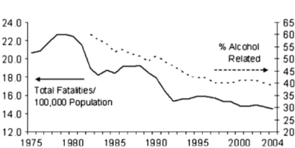
Administration (NHTSA, 2005a) reports that the number of alcohol-related traffic fatalities has fallen from 26,173 to 16,694, even as the number of miles traveled has increased by 81%. More important for measuring the effect of control legislation, the rate of alcohol involvement in fatal crashes fell from 60% in 1982 to 39% in 2004.
The good news over the past 25 yr is tem-pered, however, by slow progress in the past decade in reducing total fatalities and almost no progress in further reducing the rate of alcohol involvement. Figure 1 displays the trends in total fatalities per 100,000 popula-tion (solid line, left axis) for the years 1975– 2004 and the percentage of fatalities that are alcohol related (dotted line, right axis) for the years 1982–2004. As shown in the chart, total fatality rates were constant until 1980, fell sharply during the 1980–1982 recession, stabilized, and then fell sharply again during the period 1987–1992. After 1992, fatality rates continued to decline but at a much slower pace than in the previous decade, with the number of total traffic deaths fluctuating around 40,000 annually for the past decade.
Alcohol-related fatalities as a share of the total have only declined by 1% since 1997. Other measures of alcohol-impaired driving, including surveys of self-reported drinking and driving by the Centers for Disease Con-trol, cited in Quinlan et al. (2005), and by NHTSA (2003a), report actual increases from 1997 to 2002 in the frequency of DUI and in the number of drinks consumed when driving after drinking. These developments lead to questions regarding the effectiveness of the many types of drunk driving laws passed in recent years, including the push to reduce the BAC limit to 0.08.
Figure 2 displays the 5-yr frequencies of the adoption by the states since 1980 of two important types of alcohol control legislation, BAC laws and ALR laws. The bottom of each bar (shaded black) is the number of states adopting ALR laws during the 5-yr period, the middle (in gray) is the number adopting BAC 10 laws, and the top (in white) is the number adopting BAC 08 laws.
During the early 1980s, almost all states put BAC and/or ALR laws on the books. From the mid-1980s through the 1990s, 23 of the remaining states passed ALR laws, and another eight added BAC 10 laws. Prior to 2000, 14 added BAC 08 laws, with nine of those replacing BAC 10 laws already on the books. Thirty-two states have passed BAC 08 laws since 2000, primarily in response to federal legislation again threatening the loss of highway funding for noncompliance.2No state has passed an ALR law since 1998.
Proponents of BAC 08 laws, including MADD and NHTSA, argue that drivers with BAC 08 are ‘‘significantly impaired,’’ that the risk of a crash ‘‘rises . . . rapidly once a driver reaches or exceeds BAC 08,’’ and that the BAC 08 limit ‘‘has the potential for saving hundreds of lives and reducing thousands of serious injuries each year’’ (NHTSA, 2003b).
Others argue, however, that the lower limit unfairly penalizes moderate drinkers who are unlikely to cause crashes, while doing nothing to deter heavily intoxicated drivers who pose the more serious risk to themselves and to others. There are those who may agree that a lower standard may indeed save some lives but that the additional costs of enforcement, and the criminal penalties imposed on the marginal offender, exceed the benefits accru-ing from the law.3
The present study does not address issues of impairment but only whether or not BAC 08 laws have a measured effect on traffic fatali-ties. Like previous studies such as Dee
FIGURE 1
Traffic Deaths, United States: 1975–2004
2. South Carolina passed a BAC 10 law in 2001, sub-sequently lowered to BAC 08 in 2003; see Appendix Table A1 for the effective dates of BAC and ALR legislation for the 48 contiguous states.
3. In 2004, the latest available data total 16,694 alco-hol-related fatalities; drivers accounted for 9,462 of those killed. Drivers with 0.08 and 0.09 BACs were about 10% of the total drivers killed, or 5.8% of total alcohol-related fatalities (NHTSA, 2005b).
(2001) and Eisenberg (2003), the present study addresses this problem by using state-level traffic fatalities as the dependent variable in a pooled cross-section time series analysis. As noted by Dee and Eisenberg, the advantage of using pooled state-level data is the ability to control, through two-way fixed effects, un-observable differences across states and across time.
This article extends previous research in three important ways. First is the availability of more observations, an advantage of any later study but one that is especially critical given the relatively short time series available and the few states (five only) with BAC 08 laws as late as 1993.
Second, both driving and drinking behav-iors are habitual and persistent, and the response to new traffic laws may be attenu-ated. The present study finds strong evidence of serial correlation in the residuals of the fixed effects regressions, an indication that at the very least tests of coefficient significance in these regressions may be biased. Several cor-rections are proposed, including the use of a lagged dependent variable (LDV) model, the use of ‘‘randomized inference’’ proposed by Bertrand, Duflo, and Mullinainthan (BDM) (2004) to bootstrap empirical distribu-tions for standard errors of the coefficients of ‘‘differences-in-differences’’ estimates, and the use of an alternative estimator also proposed by BDM that essentially ignores the time series properties of the data.
Third, this study is also the first to distin-guish between early state adopters of the BAC 08 standard, which did so apparently on own initiative, and late state adopters (post-1999), at least some of which did so under pressure of the loss of federal highway
funds.4Because endogeneity is an ever-present concern in measuring the effects of legisla-tion—laws, after all, are usually passed in response to something, either from a change in public mood and/or from a need to address a public policy concern—the imposition of a federal mandate may serve as a natural exper-iment for late adopters of BAC 08.
This research employs event study method-ology to test endogeneity bias. With an event study, a period prior to the ‘‘event’’—in this case, a new alcohol control law—is used to estimate a baseline model. The model is used to make predictions over the event window, a period surrounding the effective date of the law.5Large positive or negative prediction errors prior to the effective date may indicate that the law’s passage is not independent of the public’s attitudes or behaviors. Depending on the pattern of the errors, the event study meth-odology may also provide some evidence as to the source of any endogeneity.6
The results of pooled regressions corrected for serial correlation and event analyses indi-cate that the marginal effect of strengthening BAC laws from 0.10 to 0.08 has had little to no effect on traffic fatalities, whether measured in total or restricted to times and days when alco-hol-related crashes are most likely. Indeed, the inclusion of more recent fatality data calls into question the efficacy of BAC laws at any level. On the other hand, consistent and significant reductions in fatalities follow ALR laws. Because ALRs almost always use a BAC limit as a criterion, however, the results are properly interpreted as a partial effect conditioned on the existence of a BAC law.
The article also finds robust support for pri-mary enforcement of seat belt laws and reduc-tion of highway speed limits below 70 miles per hour (mph) as fatality-reducing measures
FIGURE 2
Timing of Alcohol Laws
4. Quoting Governor Janet Hull as she signed Arizo-na’s BAC 08 law into effect: ‘‘I hate to be blackmailed by them [Congress], but we cannot in this state, which is so fast growing, afford to pass on road money’’ (Thomsen, 2001).
5. In this article, the estimation period stops 3 yr prior to the enactment of the law, and the event window is the
event year +/2 yr.
6. Eisenberg (2003) is an exception to previous research in using a series of binary variables to test pre-and postpolicy effects pre-and finds some evidence of a decrease in fatalities prior to the enactment of BAC 08 laws (but not prior to ALR laws), suggesting the pos-sibility of an unobserved influence jointly on policy and driving habits. His treatment does not address serial cor-relation and the problem of potential bias in the standard errors of binary coefficients, however.
but only mixed support for graduated driver’s license programs (GDL) in reducing total fatal-ities. Other work, including Dee, Grabowski, and Morrisey (2005), has shown GDL to be effective in reducing fatalities among 15- to 17-year-olds.
The article is organized as follows: Section II provides a brief review of the literature, Sec-tion III describes the data and methodology, Section IV provides the pooled regression results with corrections for serial correlation and the event study, and Section V concludes.
II. PREVIOUS RESEARCH ON ALCOHOL CONTROL LEGISLATION
There is a voluminous literature on alcohol control legislation. This selective review emphasizes studies focusing on, or at least with substantial coverage of, BAC 08 laws and studies appearing subsequent to legisla-tion passed in the early 1980s.
Zador et al. (1989) review the effects of three types of control legislation: BAC laws, ALR laws, and mandatory first-offense jail sentence laws, all enacted by states between 1975 and 1985. The Zador’s analysis compares changes in fatalities in states with legislation (the treatment group) to those in contiguous states without legislation (the control group). Although all three types of legislation were found to contribute to reductions in fatalities, the effects were small and only ALR laws were consistently significant across types of crashes and drivers.
NHTSA (1994) noted improvement in several measures of alcohol-related fatalities following enactment of BAC 08 laws in five states (California, Maine, Oregon, Utah, and Vermont), all with preexisting BAC 10 laws. In an independent study of the same states, Hingson, Heeren, and Winter (1996) also found significant effects of BAC 08 laws.
Voas et al. (2000) evaluate the implementa-tion of BAC 08 in 1997 in Illinois. None of Illi-nois’ bordering states had passed a BAC 08 law by 1997, so these were thought to be good controls. Voas et al. find that the ratio of drinking to nondrinking drivers fell in the 18 mo following the enactment of Illinois’ BAC 08 law, and a follow-up study by NHTSA (2001) found a continued reduction in the subsequent year (for a total of 30 mo of data). It is not clear, however, whether the BAC 08 law had a permanent effect on
alcohol-related fatalities or whether the mea-sured effects were only short-term reactions to other factors like publicity surrounding the new law or greater enforcement efforts during the year or so after enactment.
In a meta-analysis, the U.S. General Accounting Office (GAO, 1999) evaluated seven government-sponsored studies of BAC 08 laws (five by NHTSA, a strong proponent of BAC 08 laws), concluding that the ‘‘. . .
studies fall short of finding conclusive evi-dence that 0.08 BAC laws by themselves have been responsible for reductions in traffic crashes’’ (GAO, p. 23). The GAO did find some evidence of BAC 08 law effectiveness when combined with other laws and efforts at public education, but any effects depended on a number of other factors that were not controlled within the studies they examined, including levels of law enforcement, other laws in effect, and public attitudes.
Dee (2001) addresses some of the method-ological shortcomings of previous studies by regressing pooled time series of state-level traf-fic fatalities against traftraf-fic legislation and state economic controls. State and year fixed effects control for unobserved heterogeneity in traffic fatalities across states and time. The time ef-fects control for improved automotive safety, changing national attitudes, legislation toward drunk driving, and other common time-vary-ing but unobserved factors. The state effects control for cross-state differences in unobserv-able factors such as enforcement levels, traffic conditions, liquor laws, and so on. Using a technique commonly termed differences-in-differences, wherein indicator variables are used to discriminate states that pass BAC 08 laws during the sample period (the ‘‘treat-ment’’ group) from those that do not (the ‘‘control’’ group), Dee finds that the presence of a BAC 08 law reduces total traffic fatalities by 7.2% in his preferred specification, control-ling for the effects of other traffic laws and for the state-specific business cycle.
Using a similar differences-in-differences approach, Eisenberg (2003) tests directly and finds evidence confirming the hypothesis that the marginal effect of BAC 08 over BAC 10 laws is statistically significant and amounts to about an additional 2% reduction in fatalities. Eisenberg also tests for timing effects of BAC 08 laws and finds that there is some evidence of delayed response (up to 6 yr) to lower BAC limits, as well as evidence
indicating that fatalities had begun to fall in advance of the law’s effective date, suggesting endogeneity in the passage of the BAC 08 law. Eisenberg’s results are heavily dependent on just seven states that set the lower limits in the 1983–1993 period, however. Eisenberg finds little support, moreover, that ALR laws reduce fatalities in most specifications but does find that graduated license laws have been effective in reducing fatalities in under-age drivers.
In general, studies that focus on single states and/or groups of states tend to find only mixed support for the position that BAC 08 laws have an effect on traffic fatalities beyond that of existing BAC 10 and ALR sanctions. Studies using pooled time series cross-sections of state-level data tend to show stronger ef-fects for BAC 08 laws.
BDM (2004) show, however, that standard errors in differences-in-differences models can be biased by serial correlation. In what fol-lows, we reexamine the state-level data on traf-fic fatalities and alcohol laws using the differences-in-differences methodology using more recent data, test for serial correlation, and apply various corrections to coefficient standard errors. We also examine more closely the issue of the endogeneity of the laws them-selves using event analysis to pin down the timing of the legislation relative to changes in fatality rates.
III. DATA AND METHODOLOGY
A. Data
Fatality data are compiled from the Fatal-ity Analysis Reporting System (FARS) administered by NHTSA7. FARS compiles data on all traffic crashes that result in the death of a vehicle occupant or a nonmotorist. The data are gathered by state employees using a standard format for comparability across jurisdictions. Each record contains
information on date, time, day of week, road conditions, age of victim, age of driver(s), number of vehicles, vehicle speed, and many other crash attributes.
The dependent variable in the empirical analyses to follow is the rate of traffic fatalities per 100,000 population at the state level over the years 1980–2004 for the 48 contiguous states. The FARS is used to generate fatality rates for total, weekend night, and multiple daytime crashes. Ideally, alcohol-related crashes would be used for a test of alcohol con-trol laws but only since 1982 has a consistent methodology been established for counting alcohol-related traffic deaths, and even now there are wide variations across states in the proportion of drivers tested, alive or dead (Yi et al., 1999).
Because the rate of alcohol involvement is almost four times higher in nighttime crashes and over twice as high during the weekend (NHTSA, 2005b), crashes in ‘‘peak times’’— weekend nights—are used as proxies for alcohol-related deaths. In contrast, multiple-vehicle daytime crashes have an especially low rate of alcohol involvement, so a priori
we should expect alcohol control legislation to have smaller effects on these crashes.8
The independent variables include indi-cator variables for control legislation, includ-ing BAC, ALR, GDL, seat belt, and speed limit laws. Other controls include continuous variables for the business cycle, mileage trav-eled, and demographic characteristics. The included controls, in particular those in-dicating the existence or absence of a specific alcohol-related statute, are by no means ex-haustive, but as most of the variation in the model is explained by the state- and time-spe-cific effects and as the baseline results for the variables of main interest are comparable to previous research, the included controls were limited in the interest of parsimony. Descrip-tive statistics for all variables are listed in Table 1.
As shown in Table 1, both total and week-end night traffic fatality rates have fallen over time, with weekend night rates declining about twice as fast. The dispersion of weekend night
7. Data on alcohol-related traffic legislation for the years 1982–1999 were kindly provided by Thomas Dee. Earlier data on legislation were taken from Zador et al. (1989) and later data on legislation and all fatality data from the National Center for Statistics and Analysis at the NHTSA Web site at http://www-nrd.nhtsa.dot.gov/ departments/nrd-30/ncsa/. Data on graduated drivers’ licenses were taken from Dee, Grabowski, and Morrisey (2005). State unemployment rates were from Dee and the Bureau of Labor Statistics; age data were from the Bureau of the Census. All data used in this article are available on request.
8. Fifty-one percent of nighttime fatalities are alcohol related, versus 13% of daytime fatalities. Forty-three per-cent of weekend fatalities and 23% of weekday fatalities are alcohol related, as are 57% of weekend nighttime fatal-ities. Only 7% of multiple-vehicle daytime crashes are alco-hol related (NHTSA, 2005b).
rates as measured either by the range or by the standard deviation has also diminished faster than total rates, perhaps reflecting the greater uniformity of alcohol control laws across states.
The unemployment rate measures business cycle activity and has been associated by Ruhm (1996) and others with procyclicality in traffic deaths. Vehicle miles traveled ac-counts for traffic intensity, given the popula-tion level, and is positively related to fatality rates. The percentage of the population 14–24 years old controls for the demographic seg-ment with less driving experience and more risky behavior. Drivers in this age bracket are twice as likely to be involved in a fatal acci-dent as the rest of the driving population.
The indicator variables are coded 0 or 1 for states that have not or have enacted the described traffic control law, respectively.9 Only 18 states had enacted BAC laws in 1982, all with maximum limit of 0.10. By the end of 2004, all states had enacted BAC laws, with 47 at the lower limit of 0.08.10 No states had enacted ALR laws in 1982; by 2004, 39 states had enacted these laws. Seat belt laws were nonexistent in 1982; by 2004, 13 states had laws allowing penalties for not wearing a seat belt only (primary enforcement)
TABLE 1
Descriptive Statistics for Variables Used in the Analyses
Continuous Variable Year Mean
Standard
Deviation Maximum Minimum
Total fatalities per 100,000 population
1982 2.09 0.67 4.23 (New Mexico) 1.10 (Rhode, Illinois)
2004 1.67 0.63 3.24 (Wyoming) 0.74 (Massachusetts)
Weekend night per 100,000 population
1982 0.59 0.18 1.33 (New Mexico) 0.34 (Massachusetts)
2004 0.36 0.14 0.73 (Mississippi) 0.33 (New York)
Unemployment rate 1982 9.3 2.3 15.5 (Michigan) 5.5 (South Dakota)
2004 5.0 1.0 7.5 (Michigan) 3.4 (North Hampshire)
Vehicle miles traveled (billions)
1982 33.0 32.3 170.3 (California) 4.0 (Vermont)
2004 61.4 61.6 329.0 (California) 7.6 (North Dakota)
Population aged 14–24 (%) 1982 18.1 0.8 19.5 (South Carolina) 16.0 (Florida)
2004 14.3 1.0 18.9 (Utah) 12.5 (Florida)
Indicator Variable Year Number of States Adopting
BAC 08 1982 0 2004 47 BAC 10 1982 18 2004 1 ALR 1982 0 2004 39 Seat belt (primary enforcement) 1982 0 2004 13 Seat belt (secondary enforcement) 1982 0 2004 34
Graduated driver’s license 1982 0
2004 40
Maximum speed limit 70+
1982 0
2004 18
Notes:Fatality data are from the Fatality Analysis Reporting System (FARS) compiled by NHTSA. Data on traffic
legislation for the years 1982–1999 were kindly provided by Thomas Dee. Earlier data on legislation were taken from Zador et al. (1989) and later data on legislation from the National Center for Statistics and Analysis at the NHTSA Web site at http://www-nrd.nhtsa.dot.gov/departments/nrd-30/ncsa/. Data on graduated drivers’ licenses are taken from Dee, Grabowski, and Morrisey (2005). State unemployment rates are from Dee and the Bureau of Labor Statistics; age data are from the Bureau of the Census.
9. For states enacting the law within the year, the vari-able is coded for the fraction of the time the law was in force.
10. As of August 2005, all states, including the District of Columbia, have 0.08 limits.
and 34 more allowing penalties for not wear-ing a seat belt when stopped for some other violation (secondary enforcement). GDL for youth drivers were nonexistent before 1996; by 2004, 40 states had some variant of GDL. Finally, all states followed the federally mandated 55 mph maximum speed limit in 1982; by 2004, 18 states had maximum limits at 70 mph or above.11
B. Methodology
The initial methodology to be employed is a two-way fixed effects specification of the pooled time series cross-section regressions of state fatality rates on the indicator and con-tinuous variables of the form:
yit5liþstþc#Litþu#Xitþeit; ð1Þ
whereyitis an annual fatality rate for stateiin
yeart,t51,. . .,T,liis the state fixed effect,st
is the year time effect,Litis a vector of
indica-tor variables with values of 1 for the years in which the laws were in effect and 0 otherwise, and Xit is a vector of control variables. The
coefficients ofLitare often described as
differ-ences-in-differences estimators; that is, the coefficient estimates the difference in the mean of the dependent variable of the treatment group before and after the passage of the law, less the same quantity for the control group.
Correct inference using Equation (1) re-quires that the error term, eit, be i.i.d. and
uncorrelated with the regressors. There are at least two reasons to suspect that these requirements are not met. First, persistence in driving and drinking habits, combined with the construction of the indicator variables, is likely to result in serially correlated errors and therefore biased significance tests of the coefficients. Second, the differences-in-differ-ences approach assumes random assignment of treatment and control states. As noted ear-lier, however, laws are not passed randomly.
Attitudes and behaviors may change laws or laws may change attitudes and behaviors, or both. If laws are changing in response to behaviors, the estimated coefficients in Equa-tion (1) will be inconsistent.
BDM (2004) suggest several approaches to mitigating problems of serial correlation in differences-in-differences estimators. The first is the ‘‘random inference’’ test, a Monte-Carlo type approach to calculating the empirical dis-tributions of the coefficients of the indicator variables. BDM find that random inference performed the best among several alternatives in correcting problems of overrejection in dif-ferences-in-differences estimators where auto-correlation is present.
The basic technique of random inference is straightforward. Suppose that lawLjis to be
tested. Equation (1) is estimated so as to obtain the coefficientc^j. Then, to construct the empirical distribution of cj, Equation (1)
is reestimated with ‘‘pseudolaws’’ generated randomly, using the same dates as in the orig-inal sample but assigned randomly across the states. In the control sample, for instance, there are 16 states that passed BAC 08 laws during the years 1982–1998. In the first draw, a year is chosen from the 16 + 32 possibilities (duplicate years among the 16 are included; the 32 with no law are assigned zeros). In the second draw, a state is chosen and assigned the ‘‘law’’ from the first draw (either one of the true law-years or zero). The procedure is re-peated for all 48 states, and the estimate of the pseudo-cjis made and stored. The entire
process is repeated 10,000 times to generate the empirical distribution and from the distri-bution, the empiricalpvalues. The procedure is repeated for each indicator variable in the sample.
The second alternative estimator ignores the time series information by regressing the dependent variable on state and time effects, and all control variables save the law of inter-est. Then, the residuals from the adopting states only are subjected to a means test pre-and postadoption via a two-period panel. Rejection of the null of equality indicates that the law’s effects are significant.
Finally, and as an alternative to the static fixed-effects model, we estimate a dynamic LDV model. A model of this form can be jus-tified as an application of a Koyck-type geo-metric lag in the impact of the new law on traffic fatalities.
11. Other changes in state legislation of note over the time period are the institution of a uniform minimum drinking age, 21, across all states, and the enactment of ZT laws for underage drinking while driving for all states. These actions have been shown to have effects on traffic fatalities among young drivers (see Carpenter, 2004; Kaestner, 2000) but were not found to be significant in the empirical analyses here or to cause material changes in the coefficients of the variables of interest.
Event studies, often used in the finance lit-erature to measure the effect of an economic or legal ‘‘event’’ on the value of a firm, are employed to test for endogeneity bias. The basic idea is to examine whether out-of-sample prediction errors of traffic fatality rates dis-play a discernible pattern around the time a control law is enacted. Ideally, errors will cluster around zero prior to a control law’s enactment, then turn negative thereafter. Bounds are constructed to give approximate tests of significance.
To produce the out-of-sample predictions for an event study, a state’s ‘‘normal fatality rate’’ is estimated using Equation (1) during an estimation period prior to theevent window, the latter specified as the period of interest before and after the actual event. The effect of the event is estimated by the prediction error during the event window, defined to be the actual fatality rate less the rate pre-dicted by estimates from Equation (1), or
^
mi;s, wheresdesignates the event window.
The prediction errors for all the ‘‘treated’’ states are then averaged to yield the mean pre-diction error: ms51 N XN i51 ^ mi;s ð2Þ
which has variance: r2ms5 1 N2 XN i51 r2miþ1 Li ½1þðRm;s^lmÞ2 r2 m ð3Þ wherer2
miis the estimated variance of the
resid-uals from individual state regressions [Equa-tion (2)], Li is the length of the estimation
window for state i, and l^m, r2
m are the
esti-mated mean and variance of national traffic fatalities; see MacKinlay (1997).
The mean prediction errors are then accu-mulated over the event window [s1,s2] to yield
the cumulative prediction errorcs1;s25 Ps2
s1ms, which under assumptions of normally distrib-utedmi,t, has mean zero and variance equal to
the simple sum of the variances Equation (3) over the event window.12
By examining thepatternof the cumulative prediction error, we can, for example, infer whether traffic fatalities were unusually high prior to the passage of a particular law, sug-gesting that the law was to some degree a reac-tion to a worsening problem, or had begun to decline prior to passage, indicating that the law may be in response to changed attitudes and behaviors. By using the estimatedvariance
of the mean prediction error, we can infer whether any patterns detected in the errors are statistically significant.
In addition to the issues noted above, a complicating factor in isolating the effects of any particular piece of legislation on traffic fatalities is the rapid passage of many laws in succession in many of the states. One report, for example, noted that California amended its alcohol-related traffic laws 55 times between the years 1980 and 1986 (Drivers Research Institute, 2005). The failure to pro-duce a significant estimate for a particular law may not mean the law was ineffective, only that its effects could not be separated from the effects of other legislation.
In the following section, we apply alterna-tive specifications of pooled cross-section time series estimates with corrected standard errors and event studies to identify those laws, if any, that have had a significant effect on traffic fatalities.
IV. EMPIRICAL RESULTS
A. Two-Way Fixed Effects Regressions
Table 2 presents the results of Equation (1) for different categories of traffic fatalities. Two sets ofpvalues are reported for the coef-ficients of the indicator variables, one in nor-mal face calculated via robust standard errors generated from the usual White-type correc-tion of the variance-covariance matrix and one in bold face calculated via empirical distri-butions generated using random inference.
Model A replicates approximately the results from Eisenberg (2003) and Dee (2001; Table 3, column 3).13 BAC 08, BAC 10, and ALR laws are all significant at the usual levels
12. The variance formula in (3) makes strong assump-tions about the independence of the abnormal returns both intertemporally and across states, assumptions that are likely to be violated in practice (Salinger, 1992). As will be shown below, however, this bias is not likely to affect the interpretation of the results.
13. Variables included in Dee (2001) but not included here are dram shop statutes, mandatory jail time for first offense, ZT for minors, and real personal income. None of the coefficients for these variables were significant, either in Dee (2001) or here (and their inclusion had no material effect on the coefficients of the variables in Table 2), so they were excluded in the interest of parsimony.
TABLE 2 Pooled Time Series Cross-Section Regression s o f Traffic Fatalities per 100,000 Population on Alcohol Control and Other Traffic Laws. Annual Data, 1980–2004 , Except Model A Fatality Catego ry Variab le (A) Tota l (1 982–199 8) (B) Total (C) To tal (D ) W ee kend Nights (E) Multiple Acc ident s, Daytim e BAC 08 0.029 (0.085 ) * ( 0.237 ) 0.005 (0. 654) ( 0.509 ) 0.000 (0.998 ) ( 0.718 ) 0.012 (0.478 ) ( 0.538 ) 0.009 (0.612 ) ( 0.425 ) BAC 10 0.052 (0.003 ) ** ( 0.148 ) 0.005 (0. 720) ( 0.351 ) 0.005 (0.706 ) ( 0.709 ) 0.023 (0.234 ) ( 0.469 ) 0.031 (0.130 ) ( 0.122 ) ALR 0.077 (0.000 ) ** ( 0.000 ) ** 0.080 (0. 000) ** ( 0.000 ) ** 0.069 (0.000 ) ** ( 0.001 ) ** 0.057 (0.000 ) ** ( 0.011 ) * 0.103 (0.000 ) ** ( 0.000 ) ** Seat be lt (primary ) 0.042 (0.004 ) ** ( 0.017 ) * 0.067 (0. 000) ** ( 0.030 ) * 0.044 (0.006 ) ** ( 0.030 ) * 0.024 (0.267 ) ( 0.542 ) 0.079 (0.002 ) * ( 0.033 ) * Seat be lt (sec ondary) 0.021 (0.049 ) ** 0.003 (0 .734) 0.016 (0.145 ) 0.025 (0.133 ) 0.012 (0.564 ) 70+ mph 0.040 (0.011 ) * ( 0.000 ) ** 0.063 (0 .000) ** ( 0.001 ) ** 0.045 (0.000 ) * ( 0.012 ) ** 0.045 (0.018 ) * ( 0.008 ) ** 0.020 (0.303 ) ( 0.152 ) Vehicle miles 0.012 (0.762 ) 0.038 (0. 298) 0.065 (0.127 ) 0.088 (0.161 ) 0.159 (0.010 ) ** Unemp loyed 0.026 (0.000 ) ** 0.022 (0. 00) ** 0.023 (0.00) ** 0.021 (0.000 ) ** 0.024 (0.000 ) ** Popula tion age d 14–24 0.017 (0.00) ** 0.025 (0.000 ) ** 0.007 (0.284 ) Graduat ed license 0.033 (0.001 ) ** ( 0.182 ) 0.031 (0.044 ) * ( 0.143 ) 0.038 (0.022 ) * ( 0.110 ) Adjuste d R 2 0.92 0.90 0.91 0.80 0.82 Pooled Durbin-W atson 1.01 ** 0.83 ** 0.85 ** 1.38 * 1.57 * ^q , ð S^q Þ 0.52 (0.23) Note s: p Values fr om robu st standar d errors in par entheses. p Values fr om empirical distrib utions gener ated via random infe rence in bold . ** Sign ificant at 0.05 level; * sign ifican t a t 0.10 level.
using p values derived from robust standard errors and the usual t distribution (ignore the bold p values for now). The coefficient of BAC 08 in Model A indicates that BAC 08 lim-its lower the fatality rate by an additional 2.9% beyond a BAC 10 limit, or a total of 8.1% ver-sus no BAC limit.14Seat belt laws are found to reduce fatalities; maximum speed limits of 70 mph or higher are found to increase fatalities; and traffic fatalities are found to be procyclical, all consistent with previous literature.
In Model B, the sample is extended back to 1980 and forward to 2004. Extending back to 1980 captures the years immediately prior to the first ‘‘big push’’ in alcohol control legisla-tion: in 1980, only 15 of 48 states had BAC 10 laws and none had ALR laws; by 1983, 34 of 48 states had BAC 10 laws and 14 had ALR laws. Extending the sample forward to 2004 has the obvious advantage of more observa-tions (the total sample size is increased by 47%), especially important in capturing the results of another flurry of legislation in the early to mid-1990s, as well as picking up
the states that passed BAC 08 laws in response to the threat of losing federal highway funds. In contrast to Model A, neither BAC coef-ficient is significant in the extended sample using robust standard errors.15 To see why the results are so different for the longer sam-ple, we note that over 30 states passed BAC laws during 2000–2004, even as alcohol-related traffic fatalities, as a percent of the total, were constant. In fact, of 15 states that passed BAC 08 laws between 2000 and 2002, nine had increases in total fatality rates between 2000 and 2004, and as shown below, the prediction errors for this group were unexpectedly positive on average 2 yr after BAC enactment.
ALR, primary seat belt laws, and higher speed limits remain significant and of the expected sign in the expanded sample, but the effect of secondary seat belt laws is not measurable in this or any subsequent models. Liu et al. (2006) report that the percentage of passenger vehicle occupant fatalities during 2000–2004 who were unrestrained was 51% in primary seat belt law states versus 65% in
TABLE 3
LDV Pooled Time Series Cross-Section Regressions of Traffic Fatalities per 100,000 Population on Alcohol Control and Other Traffic Laws. Annual Data, 1980–2004, Except Model F
Fatality Category Variable (F) Total (1982–1998) (G) Total (H) Weekend Nights (I) Multiple Accidents, Daytime Lagged fatalities 0.460**(0.000) 0.546**(0.000) 0.263**(0.000) 0.178**(0.000) BAC 08 0.021 (0.152) 0.002 (0.793) 0.007 (0.684) 0.004 (0.795) BAC 10 0.006 (0.706) 0.007 (0.550) 0.007 (0.726) 0.031 (0.116) ALR 0.035**(0.001) 0.028**(0.000) 0.040**(0.001) 0.087**(0.000)
Seat belt (primary) 0.025**(0.050) 0.035**(0.000) 0.038**(0.012) 0.057**(0.001)
Seat belt (secondary) 0.003 (0.743) 0.013 (0.193) 0.017 (0.286) 0.001 (0.957)
70+ mph 0.032**(0.016) 0.021**(0.033) 0.033*(0.079) 0.022 (0.271) Vehicle miles 0.045 (0.166) 0.006 (0.298) 0.018 (0.286) 0.127**(0.037) Unemployed 0.015**(0.000) 0.013**(0.000) 0.019**(0.000) 0.020**(0.000) Population aged 14–24 0.008**(0.000) 0.017**(0.004) 0.010 (0.125) Graduated license 0.008 (0.309) 0.014 (0.357) 0.032;*(0.043) AdjustedR2 0.94 0.94 0.82 0.83 Pooled Durbin-Watson 2.09 2.16 1.99 2.03*
Notes: pValues from robust standard errors in parentheses.**Significant at 0.05 level;*significant at 0.10 level.
14. In Dee (2001), indicator variables for the BAC variables are mutually exclusive. In this article, the BAC 10 indicator remains coded ‘‘1’’ when BAC 08 is enacted, so that the coefficient for BAC 08 can be inter-preted as the marginal effect of BAC 08 over BAC 10. In this way, the significance of the marginal effect can be tested directly. This interpretation seems more natural, as BAC 10 was in effect prior to BAC 08 in all states but one (Oregon).
15. A series of regressions beginning with 1982–1998 and adding 1 yr per regression through 2004 were run to attempt to identify the timing of the changes in the coef-ficient values for the BAC variables. The BAC 10 coeffi-cient declines in magnitude monotonically as each year is added, losing statistical significance by 2002. The BAC 08 coefficient actually increases in magnitude as years are added through 2000, then declines in size, becoming insig-nificant with the addition of 2003 data.
all other states. Because New Hampshire is the only state with no seat belt law, ‘‘all other states’’ in the Liu analysis effectively comprise states with secondary laws.
Model C adds an indicator variable for grad-uated driver’s license and the percentage of the population aged 14–24 yr. Young drivers have accident involvement rates twice as high as the remainder of the population; in 2004, they account for only 14% of the population but 24% of the traffic deaths. Both these variables are significant using conventional standard errors, and both have the expected sign. Those coefficients in the original set of indicator var-iables that were significant remain significant.16 Models D and E provide a robustness check on the results of the total fatality models by focusing on fatalities much more or much less likely to involve a drunk driver. For dependent variables, Model D uses weekend night fatal-ities,17when over half of fatalities are alcohol related, and Model E uses multiple-vehicle daytime fatalities, when only 7% of fatalities are alcohol related. If alcohol control laws are working as intended, we might expect to see differential effects depending on the likeli-hood of alcohol involvement in the crash.
What support the results lend to differential effects, however, is mostly in the wrong direc-tion. With the exception of the BAC 08 coef-ficient, which is insignificant in either case, the alcohol control variables all have stronger effects in the case where alcohol involvement is less likely. Only in the case of seat belt laws does evidence of differential effects go in the way expected: daytime drivers appear to be more compliant regarding seat belt laws, with lower death rates resulting.
The results of higher and lower risk cases point out that the lack of significance of the BAC variables in the total fatality model is not due to an aggregation problem involving heterogeneous effects on fatalities with differ-ent likelihoods of alcohol involvemdiffer-ent. Other
variations in the dependent variable, including daytime and nighttime fatalities, as well as fatalities classified as alcohol related by NHTSA, were estimated with similar results.18
B. Tests and Corrections for Serial Correlation
The test for serial correlation used here is the pooled Durbin-Watson, following Bhargava, Franzini, and Narendranathan (1982).19 As shown in Table 2, the null of no serial cor-relation is soundly rejected for all the static models. The average and standard deviation of first-order autoregression coefficients for the state-level residuals in Model C are given in the bottom row of the table and clearly indi-cate a high degree of correlation between sub-sequent residual terms in the model.20
Three measures are employed to correct for autocorrelation: calculating standard errors for the coefficients of the indicator variables in Table 2 using the randomized inference method of BDM (2004); reestimating the model with an LDV; and employing a resid-ual-based approach also suggested by BDM that essentially ignores the time series proper-ties of the data.
Standard errors for the coefficients of indi-cator variables in Table 2 computed via ran-dom inference are shown in bold. Although in most cases the size of the significance test is larger using the empirical standard errors, occasionally the computedpvalues will actu-ally be smaller than those that the usual t dis-tribution would indicate, reflecting the fact that even though the empirical distribution in each case has fatter tails than the t distribu-tion, it is also sometimes nonsymmetrical about zero.21
Inference on two sets of coefficients was affected by the use of the empirical standard errors: the BAC coefficients in Model A and the GDL coefficients in Models C, D, and E, all of which have p values .0.10 using
16. It is, of course, well known that the omission of a regressor that is positively correlated with an included regressor, with both being negatively correlated with the dependent variable, will cause the coefficient of the included variable to be biased downward (i.e., more neg-ative); see Greene (2000). For this reason, inclusion of additional laws as regressors, such as ZT for minors, jail time for first offender, and so on, are more likely to
weaken, not strengthen, the case for BAC limits having
sig-nificant effects.
17. A weekend night is Friday, Saturday, and Sunday, 7:00 p.m. to 5:00 a.m.
18. That is, BAC coefficients were never significant using the full sample in these alternatives. Results are not reported to save space but are available on request.
19. Similar results were found using a Lagrange Mul-tiplier–type test with the lagged residuals.
20. The mean autocorrelation coefficient is estimated
asq^5ð1=NÞPN
i51
PT
t52ðeiteit1Þ=e2it, and the standard
devi-ation is estimated as the mean squared difference between the coefficient for the individual states and the mean coef-ficient.
21. A separate random inference procedure is com-puted for each coefficient.
the empirical standard errors. ALR, primary seat belt laws, and speed limit variables remain statistically significant at conventional levels under this method.
Table 3 reproduces the model with the addition of an LDV. It is well known that coef-ficients of LDV models with fixed effects are biased (Hsiao, 2003, among many others), with the bias especially affecting the coefficient of the LDV, but the bias would be unlikely to alter the main results in the present case.
The coefficient of the LDV is about 0.50 in Models F and G and is approximately the autocorrelation coefficient computed in Model C of Table 2. The pooled Durbin-Wat-son and the estimate of q^ indicate that the residuals of Models F–I are not autocorre-lated. The BAC and GDL coefficients are insignificant at standard levels in all models, consistent with the results from corrected stan-dard errors in Table 2. ALR, seat belt laws, and speed limits of 70 mph and over remain significant in the presence of the LDV.
The impact of ALR laws is estimated in Model G to be a 2.8% reduction in fatalities in the initial year and a long-term reduction of 6.2% with a halftime to equilibrium of about 1.25 yr. It seems quite plausible that the effect of new legislation should be realized over a period of years. Information about the new penalty must be disseminated to the public, and depending on a variety of factors, including levels of income, education, and awareness of public events, this may take some time. Also, if there is a stock of chronic offenders who are relatively resistant to all but the most puni-tive measures, it will take some time for the police to apprehend them. Only after the ‘‘word gets out’’ and/or a significant number of chronic offenders have been removed from the road, will the laws work as intended.
For the third alternative, ignoring the time series information, Equation (1) was estimated omitting one indicator variable at a time. The residuals from these regressions, using treat-ment states only, were then regressed against the respective indicator variable in a modified analysis of variance. The results from this alternative are presented in Table 4.
The results in Table 4 verify that the BAC variables do not have measurable effects on traffic fatalities in any of the categories. ALR laws, primary seat belt laws, and speed limits continue to be significant in most cases, though their estimated magnitudes are reduced.
In summary, all three methods of address-ing autocorrelation in the differences-in-differ-ences model yield roughly consistent results: in no case using the full sample are the coeffi-cients of the BAC variables significant.22
In the next subsection, event analysis is used to determine to what extent endogeneity bias may affect the results determined so far and whether the effects of the BAC 08 law are dif-ferent for late adopters, who may have passed legislation under federal pressure and thus may be less likely to be affected by endogeneity con-cerns. We also examine patterns of fatalities in the years surrounding the passage of ALR laws and primary seat belt laws for comparison.
C. Event Studies of Alcohol Control Laws
The prediction errors from a variation of Equation (1) are examined to determine if there are any abnormal movements prior to or after passage of the BAC 08, ALR, and pri-mary seat belt laws and whether these move-ments exceed error bounds (by convention, two standard deviations).23To allow sufficient degrees of freedom for estimating the predic-tion equapredic-tion, only states enacting laws by 1990 or later were used.
There are 39 states with BAC 08 laws passed in 1990 or later. Of these, 13 passed laws prior to 2000, the year federal highway funding stipulations were placed on states’ adoption of BAC 08 laws. Fifteen more states passed BAC 08 laws in the years 2000–2002; these states are assumed to have done so in response to the effective federal mandate and may provide a test of the difference in effects between states that adopt laws under
22. A fourth alternative, the clustering of standard errors by state using a generalized White formula is also found to work well by BDM (2004) in correcting for seri-ally correlated errors in differences-in-differences regres-sions. However, this method does not work as well when the number of treated states is low, as are the num-ber of BAC 08 states prior to about 1994, and in view of the consistency of results in the three alternatives pre-sented in the article, is omitted in the interest of brevity. 23. Eisenberg (2003) examines the timing of BAC 08 laws using dummy variables for 2-yr periods before and after the effective dates of the laws. It is easily shown (see Greene, 2000, 308–310) that the estimated coefficients
of dummy variables for individualobservations are the
same as prediction errors for those observations (and in fact, the prediction errors in the present analysis are esti-mated this way), so Eisenberg’s method has something in common with event studies. With the ‘‘dummying out’’ of so many observations in Eisenberg’s regressions, however (all but 2 yr of data in the case of California), it is not clear what is actually being measured.
their own initiative versus states that do so under federal pressure.24In addition, 16 states passed ALR laws in 1990 or later.25 Seven states passed appear on both lists, but only California passed both a BAC 08 and an ALR law effective in the same year. Ten states passed primary seat belt laws in 1990 or after. The results of the event studies for BAC 08 laws are illustrated in Figure 3. The solid lines in the graphs are the cumulative mean predic-tion errors, and the dashed lines are two stan-dard deviation error bounds. Because the prediction errors were often quite large rela-tive to the magnitude of the dependent vari-able, also included on the chart is the net +/
count of the prediction errors for each time period along the zero axis as a robustness check against influential outliers.
For the early adopters, the cumulative aver-age prediction errors in the BAC 08 analysis are slightly negative prior to the effective date and slightly positive in the years after, but well within the error bounds throughout. The net +/errors confirm this pattern, with net neg-ative prediction errors prior to the effective year and small positives thereafter. For this group, the BAC 08 laws had no systematic effect on prediction errors given information prior to the event window.
For the 15 states in the late-adopting group, the results of the event study indicate apositive
response of fatalities to the BAC 08 law
although the cumulative errors remain within the bounds of two standard errors. This is not what one would expect to see and may indicate that states that were required to enact BAC 08 laws did not enforce them or that other un-measured factors simply overwhelmed what-ever preventative effects the law would have had.26 The issue of enforcement levels is important, of course, and is largely omitted in this and most previous work on alcohol control legislation in the economics literature. A useful next step in this literature is to incor-porate measures of enforcement to control for the variation in the likelihood of apprehension among enforcing and nonenforcing states.
By contrast, the pattern of the ALR and primary seat belt prediction errors in Figure 4 is consistent with what one would expect to see if these laws were effective. Some endogeneity in these laws’ passage, however, cannot be ruled out. Cumulative average prediction errors are slightly negative prior to the laws’ effective dates, then turn more sharply nega-tive in the effecnega-tive date and thereafter, and come quite close to the 2–standard deviation band after 2 yr. The net +/count is consis-tent with the cumulative errors, indicating that prediction errors for most states were negative immediately prior to and for 2 yr after the effective date.27 Assuming normality, the p
TABLE 4
Regressions of Traffic Fatalities per 100,000 Population on Alcohol Control and Other Traffic Laws, Ignoring Time Series Information. Annual Data, 1980–2004
Fatality Category
Variable (J) Total (K) WeekendNights Accidents, Daytime(L) Multiple
BAC 08 0.001 (0.992) 0.005 (0.624) 0.004 (0.319)
BAC 10 0.002 (0.774) 0.010 (0.393) 0.013 (0.289)
ALR 0.025**(0.000) 0.020**(0.037) 0.037**(0.000)
Seat belt (primary) 0.015*(0.068) 0.008 (0.440) 0.027**(0.033)
70+ mph 0.020**(0.012) 0.020*(0.081) 0.009 (0.442)
Notes: pValues in parentheses.**Significant at 0.05 level;*significant at 0.10 level. Coefficients are from a two-step
process: residuals from regressions like Equation (1) using all regressors but the subject variable are regressed on a indicator variable, using treatment states only.
24. States actually had until October 1, 2003, to pass BAC 08 legislation, but any state that passed legislation after 2000 is presumed to have done so in anticipation of the deadline. The year 2002 is used as a cutoff to allow
for a 5-yr event window (200262 years).
25. See Appendix Table A1 for the effective dates of state BAC and ALR legislation.
26. There is some evidence that the increased time required to process DUI suspects under BAC laws requir-ing blood tests may act as a deterrent to enforcement, espe-cially in rural counties with limited law enforcement resources (Kaufman County, Texas; Sheriff’s Depart-ment, private conversation).
27. The ‘‘8’’ in the second year after the effective
date in the ALR chart, for example, means that four states had positive prediction errors and 12 states had negative errors.
value of az-test that the cumulative ALR pre-diction error is zero in the second year after effect is 0.074.28
In summary, the event studies confirm no change in traffic fatalities for states passing BAC 08, irrespective of whether passed on own initiative or under federal pressure, and even some indication of perverse results in the latter case. By contrast, the pattern of fatalities around the passage of ALR and pri-mary seat belt laws is more what would be expected although some reverse causality may also be at play.
V. CONCLUSIONS
This article presents new evidence finding that laws lowering allowable BAC limits to 0.08 g/dL have no measurable effects on traffic
fatality rates using pooled time series of state-level data. The reason for the difference between our findings and prior research is pri-marily due to the extended sample, but there is also evidence that serially correlated distur-bances biased the results of previous inferen-tial tests toward finding a significant effect. Prediction errors using event studies show no indication of a change in fatality behavior before passage of the BAC 08 law.
By contrast, other measures, including ALR and primary seat belt laws, are shown to have consistently negative and significant effects on fatalities, even after correcting for serial correlation. Event studies confirm these findings. The evidence for graduated driver’s license laws is mixed, but this study does not directly examine youth fatalities.
Because it is so rare, however, to have ALR as a penalty withoutsomeBAC standard (only 28 state-years out of 1,200 in the sample), the analysis cannot realistically predict the efficacy of ALR laws apart from BAC limits.29Similarly, because only in one state was it the case that a BAC 08 law wasnotpreceded by a BAC 10 law, BAC 08 represents only the tightening of
FIGURE 3
Average Cumulative Prediction Errors
FIGURE 4
Average Cumulative Prediction Errors
28. No claim is made here for the accuracy of the stan-dard deviation of the cumulative prediction errors. With such a small estimation window, the variance of the pre-diction error is dominated by the estimation error of the coefficients, which also leads to serial correlation in the abnormal returns (MacKinlay, 1997). Added to the size problems are issues of cross-sectional dependence, which is very likely given the tendency for alcohol control legis-lation to be passed in waves. Thus, the error bands are intended to be merely suggestive.
29. The converse is more substantial, however; there were BAC laws without ALR laws in 381 state-years, almost one third of the sample.
an existing standard and thus represents a differ-ence in degree and not in kind.
It should not be overlooked, moreover, that these laws are complements, not substitutes; BAC laws set a standard for impaired driving, and ALR laws establish a punishment for vio-lating the standard. There are punishments besides ALR for impaired driving, of course, including fines and mandatory jail terms, with stiffer terms for repeat offenders; and there are other ways besides BAC laws to establish impairment, including the judgment of the arresting officer or forms of agility tests, but there must always be a standard and a punish-ment.
There is compelling evidence that ALR laws are effective in reducing traffic deaths when BAC standards are present, but we can-not know how effective the ALR laws would be if there were no BAC standards. But there is an argument that efforts spent to reduce allowable BACs from 0.10 to 0.08 may have been better spent encouraging nation-wide adoption of ALR sanctions on drunk drivers.
APPENDIX: EFFECTIVE DATES OF ALCOHOL CONTROL LAWS
REFERENCES
Bertrand, M., E. Duflo, and S. Mullinainthan. ‘‘How Much Should We Trust Differences-in-Differences
Estimates?’’ Quarterly Journal of Economics, 19,
2004, 249–75.
Bhargava, A., L. Franzini, and W. Narendranathan. ‘‘Serial Correlation and the Fixed Effects Model.’’
Review of Economic Studies, 49, 1982, 533–49.
Carpenter, C. ‘‘How Do Zero Tolerance Drunk Driving
Laws Work?’’ Journal of Health Economics, 23,
2004, 61–83.
Dee, T. ‘‘Does Setting Limits Save Lives? The Case of 0.08
BAC Laws.’’Journal of Policy Analysis and
Manage-ment, 20, 2001, 111–28.
TABLE A1
Effective Dates of BAC and ALR Laws, 48 Contiguous States
State BAC 10 BAC 08 ALR
Alabama ,1980 7/1995 7/1996 Arizona 7/1982 8/2001 1/1988 Arkansas 4/1983 8/2001 7/1996 California 3/1982 1/1990 7/1990 Colorado 7/1983 7/2004 7/1983 Connecticut 4/1985 7/2002 1/1990 Delaware 3/1983 7/2004 10/1982 Florida ,1980 1/1994 9/1990 Georgia 8/1983 7/2001 1/1993 Idaho 3/1984 7/1997 7/1994 Illinois ,1980 7/1997 1/1986 Indiana 8/1983 7/2001 8/1983 Iowa ,1980 7/2003 7/1982 Kansas 7/1985 7/1988 7/1993 Kentucky 1/1992 10/2000 ** Louisiana 1/1984 10/2003 1/1984 Maine ,1980 8/1988 9/1981 TABLE A1 Continued
State BAC 10 BAC 08 ALR
Maryland 5/1996 10/2001 1/1990 Massachusetts ** 6/2003 7/1994 Michigan 4/1983 10/2003 ** Minnesota ,1980 8/2005 7/1982 Mississippi 7/1983 7/2002 7/1983 Missouri ,1980 4/2001 9/1983 Montana 9/1983 4/2003 ** Nebraska ,1980 9/2001 1/1993 Nevada 7/1983 9/2003 7/1983 New Hampshire 9/1983 1/1994 7/1992 New Jersey 4/1983 1/2004 ** New Mexico 7/1984 1/1994 7/1984 New York ,1980 7/2003 ** North Carolina ,1980 10/1993 10/1983 North Dakota 7/1983 8/2003 7/1983 Ohio 4/1983 7/2003 9/1993 Oklahoma 7/1982 7/2001 4/1983 Oregon ,1980 10/1983 7/1984 Pennsylvania 1/1983 10/2003 ** Rhode Island 7/1983 7/2003 ** South Carolina 1/2001 8/2003 1/1998 South Dakota ,1980 7/2002 ** Tennessee 5/1996 7/2003 ** Texas 1/1984 9/1999 1/1995 Utah ,1980 8/1983 8/1983 Vermont ,1980 7/1991 12/1989 Virginia 7/1984 7/1994 1/1995 Washington ,1980 1/1999 7/1994 West Virginia 1/1987 2/2004 ,1980 Wisconsin 5/1982 10/2003 1/1988 Wyoming 1/1989 7/2002 7/1985
Dee, T., D. Grabowski, and M. Morrisey, ‘‘Graduated
Driver Licensing and Teen Traffic Fatalities.’’
Jour-nal of Health Economics, 24, 2005, 571–89.
Drivers Research Institute. ‘‘The Development of Califor-nia Drunk Driving Legislation.’’ 2005. Accessed August 15, 2006. http://www.dui.com/duieduca-tion/duilegislation.html.
Eisenberg, D. ‘‘Evaluating the Effectiveness of Policies
Related to Drunk Driving.’’Journal of Policy
Anal-ysis and Management, 22, 2003, 249–74.
Greene, W.Econometric Analysis. 4th ed. Upper Saddle
River, NJ: Prentice-Hall, 2000.
Hingson, R., T. Heeren, and M. Winter. ‘‘Lowering State Legal Blood Alcohol Limits to 0.08 Percent: The
Effect on Fatal Motor Vehicle Crashes.’’American
Journal of Public Health, 86, 1996, 1297–9.
Hsiao, C.Analysis of Panel Data. 2nd ed. Cambridge, UK:
Cambridge University Press, 2003.
Kaestner, R. ‘‘A Note on the Effect of Minimum Drinking
Age Laws on Youth Alcohol Consumption.’’
Con-temporary Economic Policy, 18, 2000, 315–25.
Liu, C., T. Lindsey, C. Chen, and D. Utter. ‘‘States with Primary Enforcement Laws Have Lower Fatality
Rates, ’’Research Note, DOT HS 810557, February,
2006 NHTSA.
MacKinlay, A. C. Event Studies in Economics and
Finance.Journal of Economic Literature, 35, 1997,
13–39.
Mothers Against Drunk Driving. ‘‘Alcohol-Related Laws: Full Report by Law.’’ 2005. Accessed August 15, 2006. http://www3.madd.org/laws/fulllaw.cfm.
National Highway Traffic Safety Administration.A
Pre-liminary Assessment of the Impact of Lowering the
Illegal BAC per se Limit to .08 in Five States.
Wash-ington, DC: U.S. Department of Transportation, 1994.
———.Evaluation of the Illinois .08 Law: An Update with
the 1999 FARS Data.(Report No. DOT 809 392).
Washington, DC: U.S. Department of Trans-portation, 2001.
———.National Survey of Drinking and Driving Attitudes
and Behaviors, 2001. Traffic Tech. Washington, DC:
U.S. Department of Transportation, 2003a.
———.08 BAC Illegal per se Level, Traffic Safety Facts:
Laws 1(1). Washington, DC: U.S. Department of
Transportation, 2003b.
———.Traffic Safety Facts 2004. Washington, DC: U.S.
Department of Transportation, 2005a.
———.Traffic Safety Facts: Alcohol. Report HS 809 905.
Washington, DC: U.S. Department of Transporta-tion, 2005b.
Quinlan, K., R. Brewer, P. Siegel, D. Sleet, A. Mokdad, R. Shults, and N. Flowers. ‘‘Alcohol-Impaired Driving
among U.S. Adults, 1993–2002.’’American Journal
of Preventative Medicine, 28, 2005, 346–50.
Ruhm, C. ‘‘Economic Conditions and Alcohol
Prob-lems.’’ Journal of Health Economics, 14, 1996,
583–603.
Salinger, M. ‘‘Standard Errors in Event Studies.’’Journal
of Financial and Quantitative Analysis, 27, 1992,
39–53.
Thomsen, S. ‘‘Hull Signs .08 DUI Limit into Law.’’
Asso-ciated Press Wire, April 11, 2001.
U.S. General Accounting Office.Highway Safety:
Effec-tiveness of State .08 Blood Alcohol Laws.
Washing-ton, DC: GAO, RCED-99–179. 1999.
Voas, R., E. Taylor, T. Baker, and A. Tippetts.
Effective-ness of the Illinois .08 Law. (Report No. DOT HS 809
186). Washington, DC: National Highway Traffic Safety Administration, 2000.
Yi, H., F. Stinson, G. Williams, and D. Bertolucci.Trends
in Alcohol-Related Fatal Traffic Crashes, United
States, 1975–1997. National Institute on Alcohol
Abuse and Alcoholism, Surveillance Report No. 49. Washington, DC: U.S. Department of Health and Human Services, 1999.
Zador, P., A. Lund, M. Fields, and K. Weinberg. ‘‘Fatal Crash Involvement and Law against
Alcohol-impaired Driving.’’Journal of Public Health Policy,