Bandwidth Estimation for Best-Effort Internet Traffic
Jin Cao
Statistics and Data Mining Research Bell Labs Murray Hill, NJ William S. Cleveland Department of Statistics Purdue University West Lafayette, IN Don X. Sun
Statistics and Data Mining Research Bell Labs
Abstract
A fundamental problem of Internet traffic engineering is bandwidth estimation: determining the band-width (bits/sec) required to carry traffic with a specific bit rate (bits/sec) offered to an Internet link and satisfy quality-of-service requirements. The traffic is packets of varying sizes arriving for transmission on the link. Packets can queue up and are dropped if the queue size (bits) is bigger than the size of the buffer (bits) for the queue. For the predominant traffic on the Internet, best-effort traffic, quality metrics are the packet loss (fraction of lost packets), a queueing delay (sec), and the delay probability (probability of a packet exceed-ing the delay). This article presents an introduction to bandwidth estimation and a solution to the problem for best-effort traffic for the case where the quality criteria specify negligible packet loss. The solution is a simple statistical model: (1) a formula for the bandwidth as a function of the delay, the delay probability, the traffic bit rate, and the mean number of active host-pair connections of the traffic, and (2) a random error term. The model is built and validated using queueing theory and extensive empirical study; it is valid for traffic with 64 host pair connections or more, which is about 1 megabit/sec of traffic. The model provides for Internet best-effort traffic what the Erlang delay formula provides for queueing systems with Poisson arrivals and i.i.d. exponential service times.
KEYWORDS: Queueing; Erlang delay formula; Nonlinear time series; Long-range dependence; QoS; Statistical multiplexing; Internet traffic; Capacity planning.
1
Introduction: Contents of the Paper
The Internet is a world-wide computer network; at any given moment, a vast number of pairs of hosts are transferring files one to the other. Each transferred file is broken up into packets that are sent along a path across the Internet consisting of links and nodes. The first node is the sending host; a packet exits the host and travels along a link (fiber, wire, cable, or air) to a first router node, then over a link to a second router node, and so forth until a last router sends the packet to a receiving host node over a final link.
The packet traffic arriving for transmission on an Internet link is a stream: a sequence of packets with arrival times (sec) and sizes (bytes or bits). The packets come from pairs of hosts using the link for their transfers; that is, the link lies on the path from one host to another for each of a collection of pairs of hosts. When a packet arrives for transmission on a link, it enters a buffer (bits) where it must wait if there are other packets waiting
for transmission or if a packet is in service, that is, in the process of moving out of the buffer onto the link. If the buffer is full, the packet is dropped.
A link has a bandwidth (bits/sec), the rate at which the bits of a packet are put on the link. Over an interval of time during which the traffic is stationary, the packets arrive for transmission at a certain rate, the traffic bit rate (bits/sec), which is defined, formally, to be the mean of the packets sizes (bits) divided by the mean packet inter-arrival time (sec), but this is approximately the mean number of arriving bits over the interval divided by the interval length (sec). Over the interval there is a mean simultaneous active connection load, the mean number of source-destination pairs of hosts actively sending packets over the link. The utilization of the link is the traffic bit rate divided by the bandwidth; it measures the traffic rate relative to the capacity of the link.
This article presents results on a fundamental problem of engineering the Internet. What link bandwidth is needed to accommodate traffic with a certain bit rate and ensure that the transmission on the link maintains quality-of-service, or QoS, criteria? Finding the QoS bandwidth must be faced in setting up every link on the Internet, from the low-bandwidth links connecting the computers of a home user to the high-bandwidth links of a major Internet service provider. Our approach to solving the bandwidth estimation problem is to use queueing theory and queueing simulations to build a model for the QoS bandwidth. The traffic inputs are live streams from measurements of live links and synthetic streams from statistical models for traffic streams.
Section 2 describes Internet TCP/IP transmission technology, which governs almost all computer networking today — for example, the networks of Internet service providers, universities, companies, and homes. Section 2 also describes the buffer queueing process and its affect on the QoS of file transfer.
Section 3 formulates the particular version of the bandwidth estimation problem that is addressed here, discusses why the statistical properties of the packet streams are so critical to bandwidth estimation, and outlines how we use queueing simulations to study the problem. We study “best-effort” Internet traffic streams because they are the predominant type of traffic on Internet links today. The QoS criteria for best-effort streams are the packet loss (fraction of lost packets), the queueing delay (sec), and the delay probability (probability of a packet exceeding the delay). We suppose that the link packet loss is negligible, and find the QoS bandwidth required for a packet stream of a certain load that satisfies the delay and the delay probability.
Section 4 describes fractional sum-difference (FSD) time series models, which are used to generate the synthetic streams for the queueing simulations. The FSD models, a new class of non-Gaussian, long-range dependent time series models, provide excellent fits to packet size time series and to packet inter-arrival time series. The validation of the FSD models is critical to this study. The validity of our solution to the bandwidth estimation problem depends on having traffic inputs to the queueing that reproduce the statistical properties of best-effort traffic. Of course, the live data have the properties, but we need assurance that the synthetic data do as well.
Section 5 describes the live packet arrivals and sizes and the synthetic packet arrivals and sizes that are generated by the FSD models. Section 6 gives the details of the simulations and the resulting delay data: values of the QoS bandwidth, delay, delay probability, mean number of active host-pair connections of the traffic, and traffic bit rate.
Model building, based on the simulation delay data and on queueing theory, begins in Section 7. To do the model building and diagnostics, we exploit the structure of the delay data — utilizations for all combinations of delay and delay probability for each stream, live or synthetic. We develop an initial model that relates, for each stream, the QoS utilization (bit rate divided by the QoS bandwidth) to the delay and delay probability. We find a transformation for the utilization for which the functional dependence on the delay and delay probability does not change with the stream. There is also an additive stream coefficient that varies across streams, characterizing the statistical properties of each stream. This stream-coefficient delay model cannot be used for bandwidth estimation because the stream coefficient would not be known in practice.
Next we add two variables to the model that measure the statistical properties of the streams and that can be specified or measured in practice — the traffic bit rate and the number of simultaneous active host-pair connections on the link — and drop the stream coefficients. In effect we have modeled the coefficients. The result is the Best-Effort Delay Model: a Best-Effort Delay Formula for the utilization as a function of (1) the delay, (2) the delay probability, (3) the traffic bit rate, and (4) the mean number of active host-pair connections of the traffic, plus a random error term.
Section 8 presents a method for bandwidth estimation that starts with the value from the Best-Effort Delay Formula, and then uses the error distribution of the Best-Effort Delay Model to find a tolerance interval whose minimum value provides an conservative estimate with a low probability of being too small.
Section 9 discusses previous work on bandwidth estimation, and how it differs from the work here. Section 10 is an extended abstract. Readers who seek just results can proceed to this section; those not familiar with Internet engineering technology might want to first read Sections 2 and 3.
The following notation is used throughout the article:
Packet Stream
• v:arrival numbers (number)v= 1is the first packet,v= 2is the second packet, etc.
• av :arrival times (sec)
• tv :inter-arrival times (sec)tv =av+1−av
• qv :sizes (bytes or bits).
Traffic Load
• c:mean number of simultaneous active connections (number)
• τ :traffic bit rate (bits/sec)
• γp :connection packet rate (packets/sec/connection)
• γb :connection bit rate (bits/sec/connection).
Bandwidth
• β :bandwidth (bits/sec)
• u:utilization (fraction)τ /β.
Queueing
• δ :packet delay (sec)
• ω :delay probability (fraction).
2
Internet Technology
The Internet is a computer network over which a pair of host computers can transfer one or more files (Stevens 1994). Consider the downloading of a Web page, which is often made up of more than one file. One host, the
client, sends a request file to start the downloading of the page. Another host, the server, receives the request file and sends back a first response file; this process continues until all of the response files necessary to display the page are sent. The client passes the received response files to a browser such as Netscape, which then displays the page on the screen. This section gives information about some of the Internet engineering protocols involved in such file transfer.
2.1 Packet Communications
When a file is sent, it is broken up into packets whose sizes are 1460 bytes or less. The packets are sent from the source host to the destination host where they are reassembled to form the original file. They travel along a path across the Internet that consists of transmission links and routers. The source computer is connected to a first router by a transmission link; the first router is connected to a second router by another transmission link, and so forth. A router has input links and output links. When it receives a packet from one of its input links, it reads the destination address on the packet, determines which of the routers connected to it by output links should get the packet, and sends out the packet over the output link connected to that router. The flight across the Internet ends when a final router receives the packet on one of its input links and sends the packet to the destination computer over one of its output links.
The two hosts establish a connection to carry out one or more file transfers. The connection consists of software running on the two computers that manages the sending and receiving of packets. The software executes an Internet transport protocol, a detailed prescription for how the sending and receiving should work. The two major transport protocols are UDP and TCP. UDP just sends the packets out. With TCP, the two hosts exchange control packets that manage the connection. TCP opens the connection, closes it, retransmits packets not received by the destination, and controls the rate at which packets are sent based on the amount of retransmission that occurs. The transport software adds a header to each packet that contains information about the file transfer. The header is 20 bytes for TCP and 8 bytes for UDP.
Software running on the two hosts implements another network protocol, IP (Internet Protocol), that manages the involvement of the two hosts in the routing of a packet across the Internet. The software adds a 20-byte IP header to the packet with information needed in the routing such as the source host IP address and the destination host IP address. IP epitomizes the conceptual framework that underlies Internet packet transmission technology.
The networks that make up the Internet — for example, the networks of Internet service providers, universities, companies, and homes — are often referred to as IP networks, although today it is unnecessary because almost all computer networking is IP, a public-domain technology that defeated all other contenders, including the proprietary systems of big computer and communications companies.
2.2 Link Bandwidth
The links along the path between the source and destination hosts each have a bandwidth β in bits/sec. The bandwidth refers to the speed at which the bits of a packet are put on the link by a computer or router. For the link connecting a home computer to a first router,β might be 56 kilobits/sec if the computer uses an internal modem, or 1.5 megabits/sec if there is a broadband connection, a cable or DSL link. The link connecting a university computer to a first router might be 10 megabits/sec, 100 megabits/sec, or 1 gigabit/sec. The links on the core network of a major Internet service provider have a wide range of bandwidths; typical values range from 45 megabits/sec to 10 gigabits/sec. For a 40 byte packet, which is 320 bits, it takes 5.714 ms to put the packet on a 56 kilobit/sec link, and 0.032 µs to put it on a 10 gigabits/sec link, which is about 180,000 times faster. Once a bit is put on the link, it travels down the link at the speed of light.
2.3 Active Connections, Statistical Multiplexing, and Measures of Traffic Loads
At any given moment, an Internet link has a number of simultaneous active connections; this is the number of pairs of computers connected with one another that are sending packets over the link. The packets of the different connections are intermingled on the link; for example, if there are three active connections, the arrival order of 10 consecutive packets by connection number might be 1, 1, 2, 3, 1, 1, 3, 3, 2, and 3. The intermingling is referred to as “statistical multiplexing”. On a link that connects a local network with about 500 users there might be 300 active connections during a peak period. On the core link of an Internet service provider there might be 60,000 active connections.
During an interval of time when the traffic is stationary, there is a mean number of active connectionsc, and a traffic bit rateτ in bits/sec. Letµ(t)in sec be the mean packet inter-arrival time, and letµ(q), in bits, be the mean
packet size. Then the packet arrival rate per connection isγp =c−1µ−(t)1packets/sec/connection. The bit rate per
connection isγb =µ(q)c−1µ −1 (t) =τ c
−1
bits/sec/connection. γpandγbmeasure the average host-to-host speed
hosts that use the link.
The bit rate of all traffic on the link isτ = cγb. Of course,τ ≤ β because bits cannot be put on the link at a
rate faster than the bandwidth. A larger traffic bit rateτ requires a larger bandwidthβ. Let us return to the path across the Internet for the Web page download discussed earlier. Starting from the link connecting the client computer to the Internet and proceeding though the links,τ tends to increase, and therefore, so doesβ. We start with a low bandwidth link, say 1.5 megabits/sec, then to a link at the edge of a service provider network, say 156 megabits/sec, and then to the core links of the provider, say 10 gigabits/sec. As we continue further, we move from the core to the service provider edge to a link connected to the destination computer, soτ andβ tend to decrease.
2.4 Queueing, Best-Effort Traffic, and QoS
A packet arriving for transmission on a link is presented with a queueing mechanism. The service time for a packet is the time it takes to put the packet on the link, which is the packet size divided by the bandwidthβ. If there are any packets whose transmission is not completed, then the packet must wait until these packets are fully transmitted before its transmission can begin. This is the queueing delay. The packets waiting for transmission are stored in a buffer, a region in the memory of the computer or router. The buffer has a size. If a packet arrives and the buffer is full, then the packet is dropped. As we will see, the arrival process for packets on a link is long-range dependent; at low loads, the traffic is very bursty, but as the load increases, the burstiness dissipates. For a fixed τ andβ, bursty traffic results in a much larger queue-height distribution than traffic with Poisson arrivals.
TCP, the predominant protocol for managing file transfers, changes the rate at which it sends packets with file contents. TCP increases the rate when all goes well, but reduces the rate when a destination computer indicates that a packet has not been received; the assumption is that congestion somewhere on the path has led to a buffer overflow, and the rate reduction is needed to help relieve the congestion. In other words, TCP is closed-loop because there is feedback. UDP is not aware of dropped packets and does not respond to them.
When traffic is sent across the Internet using TCP or UDP and this queueing mechanism, with no attempts to add additional protocol features to improve QoS, then the traffic is referred to as “best-effort”. IP networks are a
best-effort system because the standard protocols make an effort to get packets to their destination, but packets can be delayed, lost, or delivered out of order. Queueing delay and packet drops degrade the QoS of best-effort traffic. For example, for Web page transfers, the result is a longer wait by the user, partly because the packets sit in the queue, and partly because of TCP reducing its sending rate when retransmission occurs. Best-effort traffic contrasts with priority traffic, which when it arrives at a router, goes in front of best-effort packets. Packets for voice traffic over the Internet are often given priority.
3
The Bandwidth Estimation Problem: Formulation and Stream Statistical
Properties
3.1 Formulation
Poor QoS resulting from delays and drops on an Internet link can be improved by increasing the link bandwidth
β. The service time decreases, so if the traffic rateτ remains fixed, the queuing delay distribution decreases, and delay and loss are reduced. Loss and delay are also affected by the buffer size; the larger the buffer size, the fewer the drops, but then the queueing delay has the potential to increase because the maximum queueing delay is the buffer size divided byβ.
The bandwidth estimation problem is to choose β to satisfy QoS criteria. The resulting value ofβ is the QoS bandwidth. The QoS utilization is the value ofu = τ /β corresponding to the QoS bandwidth. When a local network, such as a company or university, purchases bandwidth from an Internet service provider, a decision on
β must be made. When an Internet service provider designs its network, it must chooseβ for each of its links. The decision must be based on the traffic load and QoS criteria.
Here, we address the bandwidth estimation problem specifically for links with best-effort traffic. We take the QoS criteria to be delay and loss. For delay, we use two metrics: a delay,δ, and the delay probability,ω, the probability that a packet exceeds the delay. For loss, we suppose that the decision has been made to choose a buffer size large enough that drops will be negligible. This is, for example, consistent with the current practice of service providers on their core links (Iyer, Bhattacharyya, Taft, McKeown, and Diot 2003). Of course, a large buffer size allows the possibility of a large delay, but setting QoS values forδandωallows us to control delay probabilistically; we will choseω to be small. The alternative is to use the buffer size as a hard limit on delay,
but because dropped packets are an extreme remedy with more serious degradations of QoS, it is preferable to separate loss and delay control, using the softer probabilistic control for delay. Stipulating that packet loss will be negligible on the link means that for a connection that uses the link, another link will be the loss bottleneck; that is, if packets of the connection are dropped, it will be on another link. It also means that TCP feedback can be ignored in studying the bandwidth estimation problem.
3.2 Packet Stream Statistical Properties
A packet stream consists of a sequence of arriving packets, each with a size. Letvbe the arrival number;v=1 is the first packet,v= 2 is the second packet, and so forth. Letav be the arrival times, lettv =av+1−avbe the
inter-arrival times, and letqvbe the size of the packet arriving at timeav. The statistical properties of the packet
stream will be described by the statistical properties oftvandqv as time series inv.
The QoS bandwidth for a packet stream depends critically on the statistical properties of thetv andqv. Directly,
the bandwidth depends on the queue-length time process. But the queue-length time process depends critically on the stream statistical properties. Here, we consider best-effort traffic. It has persistent, long-range dependent
tv andqv (Ribeiro, Riedi, Crouse, and Baraniuk 1999; Gao and Rubin 2001; Cao, Cleveland, Lin, and Sun
2001). Persistent, long-range dependenttv andqv have dramatically larger queue-size distributions than those
for independenttv andqv(Konstantopoulos and Lin 1996; Erramilli, Narayan, and Willinger 1996; Cao,
Cleve-land, Lin, and Sun 2001). The long-range dependent traffic is burstier than the independent traffic, so the QoS utilization is smaller because more headroom is needed to allow for the bursts. This finding demonstrates quite clearly the impact of the statistical properties. But a corollary of the finding is that the results here are limited to best-effort traffic streams (or any other streams with similar statistical properties). Results for other types of traffic with quite different statistical properties — for example, links carrying voice traffic using current Internet protocols — are different.
Best-effort traffic is not homogeneous. As the traffic connection loadcincreases, the arrivals tend toward Poisson and the sizes tend toward independent(Cao, Cleveland, Lin, and Sun 2002; Cao and Ramanan 2002). The reason is the increased statistical multiplexing of packets from different connections; the intermingling of the packets of different connections is a randomization process that breaks down the correlation of the streams. In other words, the long-range dependence dissipates. This means that in our bandwidth estimation study, we can expect a
changing estimation mechanism ascincreases. In particular, we expect “multiplexing gains”, greater utilization due to the reduction in dependence. Because of the change in properties withc, we must be sure to study streams with a wide range of values ofc.
4
FSD Time Series Models for Packet Arrivals and Sizes
This section presents FSD time series models, a new class of non-Gaussian, long-range dependent models (Cao, Cleveland, Lin, and Sun 2002; Cao, Cleveland, and Sun 2004). The two independent packet-stream time series — the inter-arrivals,tv, and the sizes,qv— are each modeled by an FSD model; the models are used to generate
synthetic best-effort traffic streams for the queueing simulations of our study.
There are a number of known properties of thetv andqv that had to be accommodated by the FSD models.
First, these two time series are range dependent. This is associated with the important discovery of long-range dependence of packet arrival counts and of packet byte counts in successive equal-length intervals of time, such as 10 ms (Leland, Taqqu, Willinger, and Wilson 1994; Paxson and Floyd 1995). Second, thetv and qv are non-Gaussian. The complex non-Gaussian behavior has been demonstrated clearly in important work
showing that highly nonlinear multiplicative multi-fractal models can account for the statistical properties oftv
andqv(Riedi, Crouse, Ribeiro, and Baraniuk 1999; Gao and Rubin 2001). These nonparametric models utilize
many coefficients and a complex cascade structure to explain the properties. Third, the statistical properties of the two time series change ascincreases (Cao, Cleveland, Lin, and Sun 2002). The arrivals tend toward Poisson and the sizes tend toward independent; there are always long-range dependent components present in the series, but the contributions of the components to the variances of the series goes to zero.
4.1 Solving the Non-Gaussian Challenge
The challenge in modeling tv and qv is their combined non-Gaussian and long-range dependent properties,
a difficult combination that does not, without a simplifying approach, allow parsimonious characterization. We discovered that monotone nonlinear transformations of the inter-arrivals and sizes are very well fitted by parsimonious Gaussian time series, a very simple class of fractional ARIMA models (Hosking 1981) with a small number of parameters. In other words, the transformations and the Gaussian models account for the complex multifractal properties of thetv and theqvin a simple way.
4.2 The FSD Model Class
Suppose xv forv = 1,2, . . .is a stationary time series with marginal cumulative distribution functionF(x;φ)
whereφis a vector of unknown parameters. Letx∗
v =H(xv;φ)be a transformation ofxvsuch that the marginal
distribution ofx∗
v is normal with mean 0 and variance 1. We haveH(xv;φ) = G−1(F(x;φ)), whereG(z)is
the cumulative distribution function of a normal random variable with mean 0 and variance 1. Next we suppose
x∗
vis a Gaussian time series and callx
∗
v the “Gaussian image” ofxv.
Supposex∗
v has the following form:
x∗ v = √ 1−θ sv+ √ θ nv,
where sv andnv are independent of one another and each has mean 0 and variance 1. nv is Gaussian white
noise, that is, an independent time series. svis a Gaussian fractional ARIMA (Hosking 1981)
(I−B)dsv =v+u−1
whereBsv =su−1,0< d <0.5, andvis Gaussian white noise with mean 0 and variance
σ2 = (1−d)Γ
2(1−d)
2Γ(1−2d) .
xv is a fractional sum-difference (FSD) time series. Its Gaussian image,x∗v, has two components.
√
1−θsv is
the long-range-dependent, or lrd, component; its variance is1−θ. √θis the white-noise component; its variance isθ.
Letpx∗(f)be the power spectrum of thex∗v. Then
px∗(f) = (1−θ)σ2
4 cos2(πf) 4 sin2(πf)d +θ
for 0≤ f ≤0.5. Asf → 0.5,px∗(f)decreases monotonically toθ. Asf → 0, px∗(f)goes to infinity like sin−2d(πf)
∼f−2d
, one outcome of long-range dependence. For nonnegative integer lagsk, letrx∗(k),rs(k),
andrn(k)be the autocovariance functions ofx∗v,sv, andnv, respectively. Because the three series have variance
1, the autocovariance functions are also the autocorrelation functions. rs(k)is positive and falls off likek2d−1
askincreases, another outcome of long-range dependence. Fork >0,rn(k) = 0and
Asθ → 1,x∗
v goes to white noise: px∗(f) → 1andrx∗(k) → 0fork > 0. The change in the autocovariance
function and power spectrum are instructive. Asθgets closer to 1, the rise ofpx∗(f)nearf =0 is always to
orderf−2d, and the rate of decay ofr
x∗(k)for largekis alwaysk2d−1; but the ascent ofpx∗(f) at the origin
begins closer and closer tof = 0and therx∗(k)get uniformly smaller by the multiplicative factor1−θ.
4.3 Marginal Distributions ofqv andtv
We model the marginal distribution oftv by a Weibull with shapeλand scaleα, a family with two unknown
parameters. Estimates of λare almost always less than 1. The Weibull provides an excellent approximation of the sample marginal distribution of the tv except that the smallest 3% to 5% of the sample distribution is
truncated to a nearly constant value due to certain network transmission properties.
The marginal distribution of qv is modeled as follows. While packets less than 40 bytes can occur, it is
suffi-ciently rare that we ignore this and suppose40≤qv ≤1500. First, we provide forAatoms at sizesφ(1s). . . φ(As)
such as 40 bytes, 512 bytes, 576 bytes, and 1500 bytes that are commonly occurring sizes; the atom probabilities are φ(1a). . . φ(Aa). For the remaining sizes, we divided the interval [40, 1500] bytes intoC sub-intervals using
C−1distinct break points with values that are greater than 40 bytes and less than 1500 bytes,φ1(b), . . . φ(Cb−)1.
For each of theCsub-intervals, the size distribution has an equal probability for the remaining sizes (excluding the atoms) in the sub-interval; the total probabilities for the sub-intervals areφ(1i), . . . , φ(Ci). Typically, with just 3 atoms at 40 bytes, 576 bytes, and 1500 bytes, and with just 2 break points at 50 bytes and 200 bytes, we get an excellent approximation of the marginal distribution.
4.4 Gaussian Images ofqvandtv
The transformed time seriest∗
v andq
∗
v appear to be quite close to Gaussian processes. Some small amount of
non-Gaussian behavior is still present but it is minor. The autocorrelation structure of these Gaussian images are very well fitted by the FSD autocorrelation structure.
The parameters of the FSD model are the following:
• qv marginal distribution: Aatom probabilities φ(ia) atAsizesφ
(s)
i ;C−1break pointsφ
(b)
i andC
sub-interval probabilitiesφ(ii)
• q∗
vtime dependence: fractional difference coefficientd(q)and white-noise varianceθ(q)
• t∗
v time dependence: fractional difference coefficientd(t)and white-noise varianceθ(t).
We found that thed(q)andd(t)do not depend onc; this is based on empirical study, and it is supported by theory.
The estimated values are 0.410 and 0.411, respectively. We take the value of each of these two parameters to be 0.41. We found that ascincreases, estimates ofλ,θ(q), andθ(t)all tend toward 1. This means thetv tend to a
independent exponentials, a Poisson process and theqvtend toward independence. In other words, the statistical
models account for the change in thetv andqv andcincreases that was discussed earlier. We estimated these
three parameters andαby partial likelihood methods withd(q)andd(t)fixed to 0.41. The marginal distribution
ofqv on a given link does not change withc, but it does change from link to link. To generate traffic, we must
specify the atom and sub-interval probabilities. This provides a mean packet sizeµ(q), measured in bits/packet.
5
Packet Stream Data: Live and Synthetic
We use packet stream data, values of packet arrivals and sizes, in studying the bandwidth estimation problem. They are used as input traffic for queueing simulations. There are two types of streams: live and synthetic. The live streams are from packet traces, data collection from live Internet links. The synthetic streams are generated by the FSD models.
5.1 Live Packet Streams
A commonly-used measurement framework for empirical Internet studies results in packet traces (Claffy et al. 1995; Paxson 1997; Duffield et al. 2000). The arrival time of each packet on a link is recorded and the contents of the headers are captured. The vast majority of packets are transported by TCP, so this means most headers have 40 bytes, 20 for TCP and 20 for IP. The live packet traffic is measured by this mechanism over an interval; the time-stamps provide the live inter-arrival times,tv, and the headers contain information that provides the live
sizes,qv; so for each trace, there is a stream of live arrivals and sizes.
The live stream database used in this presentation consists of 349 streams, 90 sec or 5 min in duration, from 6 Internet links that we name BELL, NZIX, AIX1, AIX2, MFN1, and MFN2. The measured streams have
negligible delay on the link input router. The mean number of simultaneous active connections,c, ranges from 49 connections to 18,976 connections. The traffic bit rate,τ, ranges from 1.00 megabits/sec to 348 megabits/sec.
BELL is a 100 megabit/sec link in Murray Hill, NJ, USA connecting a Bell Labs local network of about 3000 hosts to the rest of the Internet. The transmission is half-duplex, so both directions, in and out, are multiplexed and carried on the same link, and a stream is the multiplexing of both directions; but to keep the variable c
commensurate for all of the six links, the two directions for each connection is counted as two. In this pre-sentation we use 195 BELL traces, each 5 min in length. NZIX is the 100 megabit/sec New Zealand Internet exchange hosted by the ITS department at the University of Waikato, Hamilton, New Zealand, that served as a peering point among a number of major New Zealand Internet Service Providers at the time of data collec-tion (http://wand.cs.waikato.ac.nz/wand/wits/nzix/2/ ). All arriving packets from the input/output ports on the switch are mirrored, multiplexed, and sent to a port where they are measured. Because all connections have two directions at the exchange, each connection counts 2 as for BELL. In this presentation we use 84 NZIX traces, each 5 min in length. AIX1 and AIX2 are two separate 622 megabit/sec OC12 packet-over-sonet links, each carrying one direction of the traffic between NASA Ames and the MAE-West Internet exchange. In this presen-tation we use 23 AIX1 and 23 AIX2 traces, each 90 sec in length. AIX1 and AIX2 streams were collected as part of a project at the National Laboratory for Applied Network Research where the data are collected in blocks of 90 sec (http://pma.nlanr.net/PMA ). MFN1 and MFN2 are two separate 2.5 gigabit/sec OC48 packet-over-sonet links on the network of the service provider Metropolitan Fiber Network; each link carries one direction of traf-fic between San Jose, California, USA and Seattle, Washington, USA. In this presentation we use 12 MFN1 and 12 MFN2 traces, each 5 min in length.
The statistical properties of streams, as we have stated, depend on the connection loadc, so it is important that the time interval of a live stream be small enough thatcdoes not vary appreciably over the interval. For any link, there is diurnal variation, a change incwith the time of day due to changes in the number of users. We chose 5 minutes to be the upper bound of the length of each stream to ensure stationarity. BELL, NXIZ, MFN1, and MFN2 streams are 5 min. AIX1 and AIX2 traces are 90 sec because the sampling plan at these sites consisted of noncontiguous 90-sec intervals.
5.2 Synthetic Packet Streams
The synthetic streams are arrivals and sizes generated by the FSD models fortv andqv. Each of the live streams
is fitted by two FSD models, one for thetv and one for theqv, and a synthetic stream of 5 min is generated by
the models. The generatedtvare independent of the generatedqv, which is what we found in the live data. The
result is 349 synthetic streams that match the statistical properties collectively of the live streams.
6
Queueing Simulation
We study the bandwidth estimation problem through queueing simulation with an infinite buffer and a first-in-first-out queueing discipline. The inputs to the queues are the arrivals and sizes of the 349 live and 349 synthetic packet streams described in Section 5.
For each live or synthetic stream, we carry out 25 runs, each with a number of simulations. For each run we pick a delayδand a delay probabilityω; simulations are carried out to find the QoS bandwidthβ, the bandwidth that results in delay probability ωfor the delayδ. This also yields a QoS utilizationu =τ /β. We use 5 delays — 0.001 sec, 0.005 sec, 0.010 sec, 0.050 sec, 0.100 sec — and 5 delay probabilities — 0.001, 0.005, 0.01, 0.02, and 0.05 — employing all 25 combinations of the two delay criteria. For each simulation of a collection, δ is fixed a priori. We measure the queueing delay at the arrival times of the packets, which determines the simulated queueing delay process. From the simulated process we find the delay probability for the chosenδ. We repeat the simulation, changing the trial QoS bandwidth, until the attained delay probability approximately matches the chosen delay probabilityω. The optimization is easy becauseωdecreases as the trial QoS bandwidth increases for fixedδ.
In the optimization, we do not allow the utilization to go above 0.97; in other words, if the true QoS utilization is above 0.97, we set it to 0.97. The reason is that we use the logit scale,log(u/(1−u)), in the modeling; above about 0.97, the scale becomes very sensitive to model mis-specification and the accuracy of the simulation, even though the utilizations above 0.97 for practical purposes are nearly equal. Similarly, we limit the lower range of the utilizations to be 0.05.
The result of the 25 runs for each of the 349 live and 349 synthetic streams is 25 measurements, one per run, of each of five variables: QoS utilizationu, delayδ, delay probabilityω, mean number of active connectionsc, and
bit rateτ. The first three variables vary from run to run; the last two variables are the same for the 25 runs for a stream because they measure the stream statistical properties. By design, the range ofδ is 0.001 sec to 0.100 sec, and the range of ωis 0.001 to 0.05. The range of the QoS utilizations is 0.05 to 0.97. The two additional variablesτ andc, which measure the statistical properties of the streams, are constant across the 25 runs for each stream. cranges from 49 connections to 18,976 connections, andτ ranges from 1.00 megabits/sec to 348 megabits/sec.
7
Model Building: A Bandwidth Formula Plus Random Error
This section describes the process of building the Best-Effort Delay Model, which is the Best-Effort Delay Formula plus random error. The model describes the dependence of the utilizationuon the delayδ, the delay probability ω, the traffic bit rateτ, and the expected number of active connections c. The modeling process involves both theory and empirical study, and establishes a basis for the model.
The theoretical basis is queueing theory. The empirical basis is the delay data from the queueing simulations, the measurements of the five variables described in Section 6. The following notation is used for the values of these five variables for either the live delay data or the synthetic delay data. δj, forj= 1 to 5, are the 5 values of
the delay in increasing order, andωk, fork=1 to 5, are the 5 values of the delay probability in increasing order. uijkis the QoS utilization for delayδj, delay probabilityωk, and streami, wherei= 1 to 349. τi is the traffic
bit rate andciis the mean number of active connections, both for streami.
7.1 Strategy: Initial Modeling of Dependence onδandω
The structure of the data provides an opportunity for careful initial study of the dependency of theuijkonδjand ωk. We have 25 measurements of each of these variables for each streami, and for these measurements, bothτi
andciare constant. We start our model building by exploiting this opportunity.
We will consider modeling each stream separately, but hope there will be model consistency across streams that allows simplification. If such simplicity is to occur, it is likely that it will require a monotone transformation of theuijkbecause they vary between 0 and 1. So we begin, conceptually, with a model of the form
Theijkare a sample from a distribution with mean 0. f is a monotone function ofu, andgiis a function ofδ
andω; we want to choosef to makegias simple as possible, that is, vary as little as possible withi.
7.2 Conditional Dependence ofuonδ
We start our exploration of the data by takingf(u) = uand suppose that a logical scale forδ is the log. In all cases, we use log base 2 and indicate this by writinglog2in our formulas. We do not necessarily believe that this identity function forfis the right transformation, but it is helpful to study the data initially on the untransformed utilization scale.
Our first step is to explore the conditional dependence ofuijk onlog2(δj)givenωk and the streamiby trellis
display (Becker, Cleveland, and Shyu 1996). For each combination of the delay probabilityωkand the streami,
we graphuijkagainstlog2(δj). We did this once for all 349 live streams and once for all 349 synthetic streams.
Figure 1 illustrates this by a trellis display for 16 of the live streams. The 16 streams were chosen to nearly cover the range of values of theτi. Letτ(v), forv= 1 to 349, be the values ordered from smallest to largest, and take
τ(v)to be the quantile of the empirical distribution of the values of orderv/349. Then we chose the 16 streams
whose ranksv yield orders the closest to the 16 equally-spaced orders from 0.05 to 0.95. On the figure, there are 80 panels divided into 10 columns and 8 rows. On each panel,uijkis graphed againstlog2(δj)for one value
ofωk and one stream; the strip labels at the top of each panel give the value ofωk and the rank of the stream.
There are 5 points per panel, one for each value oflog2(δj).
Figure 1 shows a number of overall effects ofτ,δ, andω onu. For each pair of values ofωandτ, there is an increase inu withδ, a strong main effect in the data. In addition, there is an increase with τ for fixedδ and
ω, another strong main effect. There is also a main effect for ω, but smaller in magnitude than for the other two variables. The dependence ofuonlog2(δ)is nonlinear, and changes substantially with the value ofτ; asτ
increases, the overall slope in uas function oflog2(δ)first increases and then decreases. In other words, there is an interaction betweenlog2(δ)andτ. Such an interaction complicates the dependence, so we search further for a transformationf ofuthat removes the interaction. This pattern occurs when all of the live streams or all of the synthetic streams are plotted in the same way.
for change as a function oflog2(δ). For this reason, we tried expanding the scale at 1 by taking the function
f(u) = log2(1−u). This did not achieve appreciably greater simplicity because nonlinearity and an interaction are still strongly present, but the interaction cause is behavior for smaller values ofτ.
The nature of the remaining interaction forf(u) = log2(1−u) suggests that a logit transformation might do better: f(u) =logit2(u) = log2 u 1−u .
Figure 2 plots logit2(uijk)againstlog2(δj)using the same streams and method as Figure 1. The logit function
greatly simplifies the dependence. The dependence on log2(δ) is linear. There does not appear to be any remaining interaction among the three variables: log2(δ), τ, andω. To help show this, 16 lines with different intercepts but the same linear coefficient, have been drawn on the panels. The method of fitting will be described shortly. The lines provide an excellent fit.
7.3 Theory: The Classical Erlang Delay Formula
The packet arrivalsaj are not Poisson, although they to tend toward Poisson as candτ increase. The packet
sizes, and therefore the service times, are not independent exponential; the packet sizes have a bounded discrete distribution and are long-range dependent, although they tend to independent ascandτ increase. Still, we will use, as a suggestive case, the results for Poisson arrivals and i.i.d. exponential service times to provide guidance for our model building. Erlang showed that for such a model, the following equation holds (Cooper 1972):
ω=ue−(1−u)βδ.
Substituting forβ=τ /uand taking the negative log of both sides we have
−log2(ω) =−log2(u) + log2(e)1−u
u δτ. (1)
Because ω, which ranges from 0.001 to 0.05, is small in the majority of our simulations compared withu, we have, approximately,
−log2(ω) = log2(e)1−u
u δτ.
Taking logs of both sides and rearranging we have
So certain aspects of the simplicity of this classical Erlang delay formula occur also in the pattern for our much more statistically complex packet streams. In both cases, logit2(u)is additive in functions ofτ,δ, andω, and the dependence is linear inlog2(δ).
7.4 Conditional Dependence ofuonω
The approximate Erlang delay formula suggests that we try the term−log2(−log2(ω)), the negative comple-mentary log ofω, in the model. In addition, as we will see in Section 9, certain asymptotic results suggest this term as well. We studied the dependence of logit2(u)on−log2(−log2(1−ω))for all synthetic and live streams
using trellis display in the same way that we studied the dependence onlog2(δ). Figure 3 is a trellis plot using the same 16 live streams as in Figure 2. On each panel, logit2(uijk)is graphed against−log2(−log2(ωk))for
one value ofδj and one stream.
Figure 3 shows that the guidance from the Erlang formula is on target; logit2(u)is linear in−log2(−log2(ω)), and the slope remains constant across streams and across different values ofδ. To help show this, lines with the same linear coefficient but different intercepts, have been drawn on the panels. The lines provide an excellent fit except for the errant points for high utilizations observed earlier. The method of fitting will be described shortly. This pattern occurs when all of the live streams or all of the synthetic streams are plotted in the same way.
A Stream-Coefficient Delay Model
The empirical findings in Figures 2 and 3 and the guidance form the Erlang Delay Formula have led to a very simple model that fits the data:
,logit2(uijk) =µi+oδlog2(δj) +oω(−log2(−log2(ωk))) +ijk (3)
where the ijk are realizations of an error random variable with mean 0 and median absolute deviationm().
Theµiare stream coefficients; they change with the packet streamiand characterize the statistical properties of
the stream.
We fitted the stream-coefficient delay model of Equation 3 twice, once to the 349 live streams and once to the 349 synthetic streams; in other words, we estimated the coefficients µi, oδ, and oω twice. Data exploration
estimation (Mosteller and Tukey 1977). The estimates ofoδandoωare
Live: ˆoδ= 0.411 ˆoω= 0.868
Synthetic: oˆδ = 0.436 ˆoω = 0.907.
The two sets of estimates are very close in the sense that the fitted equation is very close, that is, results in very similar fitted QoS utilizations. For the 16 streams shown in Figures 2 and 3, the lines are drawn using the formula in Equation 3 with the bisquare parameter estimates —oˆδ,oˆω, andµˆi.
Because of the long-tailed error distribution, we use the median absolute deviation, m, as a measure of the
spread. The estimates from the residuals of the two fits are
Live: mˆ() = 0.210
Synthetic: mˆ() = 0.187.
The estimates are very small compared with the variation in logit2(u). In other words, the stream-coefficient delay model provides a very close fit to the logit2(uijk). Of course, this was evident from Figures 2 and 3
because the fitted lines are quite close to the data.
7.5 Strategy: Incorporating Dependence onτ andcfor Practical Estimation
The coefficientµiin the stream-coefficient delay model of Equation 3 varies with the packet stream and reflects
how the changing statistical properties of the streams affect the QoS utilization. Part of the simplicity of the model is that a single number characterizes how the statistical properties of a stream affect the QoS bandwidth. However, the model cannot be used as a practical matter for bandwidth estimation because it requires a value of
µ, which would not typically be known. If we knew details of the traffic characteristics in detail for the link, for example, if we had FSD parameters, we could generate traffic and run simulations to determineµand therefore the bandwidth. This might be possible in certain cases, but in general is not feasible.
What we must do is start with Equation 3, and find readily-available variables that measure stream statistical properties and can replace µin the stream-coefficient delay model. We carry out this task in the remainder of this section. Two variables replace µ, the bit rate τ and the mean number of active connectionsc, with their values ofτiandcifor each of our packet streams. We will use both theory and empirical study, as we did for the
7.6 Theory: Fast-Forward Invariance, Rate Gains, and Multiplexing Gains
Figures 2 and 3 show that the QoS utilizationuincreases withτ. There are two causes: rate gains and multiplex-ing gains. Becausecis positively correlated withτ,uincreases withcas well. But τ andcmeasure different aspects of the load, which is important to the modeling. τ is equal tocγb whereγb is the connection bit rate in
bits/sec/connection. γb measures the end-to-end speed of transfers.cmeasures the amount of multiplexing. An
increase in either increasesτ.
First we introduce fast-forwarding. Consider a generalized packet stream with bit rateτ input to a queue without any assumptions about the statistical properties. The packet sizes can be any sequence of positive random variables, and the inter-arrivals can be any point process. Suppose we are operating at the QoS utilization
u = τ /β for QoS delay criteria δ and ω. Now for h > 1, we speed up the traffic by dividing all inter-arrival times tv by h. The packet stream has a rate change: the statistical properties of the tv change only by
a multiplicative constant. A rate increase ofhincreasesγb by the factorhbut notc. The bit rateτ changes to hτ. Suppose we also multiply the bandwidthβbyh, so that the utilizationuis constant. Then the delay process of the rate-changed packet stream is the delay process for the original packet stream divided by h. That is, if we carried out a simulation with a live or synthetic packet stream, and then repeated the simulation with the rate change, then the delay of each packet in the second simulation would be the delay in the first divided byh. The traffic bit rate, the bandwidth, and the delay process are speeded up by the factorh, but the variation of the packet stream and the queueing otherwise remain the same. If we changed our delay criterion fromδ toδ/h, then the QoS utilizationuwould be the same, which means the QoS bandwidth ishβ. It is as if we videotaped the queueing mechanism in the first simulation and then produced the second by watching the tape on fast forward with the clock on the tape player running faster by the factorh as well; we will call this phenomenon fast-forward invariance.
Let us now reduce some of the speed-up of the fast forwarding. We will divide thetv byhwhich increasesγb
by the factorh. But we holdδfixed and do not decrease by the factor1/h. What is the new QoSuthat satisfies the delay criteriaδ andω? Sinceusatisfies the criteria for delayδ/h, we have room for more delay, soucan increase. In other words, a rate increase results in utilization gains for the sameδ. This is the rate gain.
the factor1/h. Now the statistical properties change in other ways due to the increased multiplexing. As we have seen in Section 4, thetvtend toward Poisson and theqvtend toward independence. The dissipation of the
long-range dependence of the packet streams, as well as the tendency of the marginal distribution oftv toward
exponential, tends to decrease the queueing delay distribution and thereby increase the QoS utilization. In other words, there are statistical multiplexing gains.
These theoretical considerations lead us to two important conclusions about modeling. First, we want to be sure that whatever model results, it must obey the principle of fast-forward invariance. Second, it is unlikely that it will be enough to model with justτ. Ifγbwere constant across the Internet,τ andcwould measure exactly the
same thing for our purposes and we would have no need forcbeyondτ. But ifγbchanges substantially, as seems
likely, then we will needcas well. Figure 4 shows the 6 medians from the 349 values oflog2(γb)for our live
streams broken up into 6 groups by the link. The range of the medians is about 4 log base 2 bits/sec/connection, which means that the medians of γb change by a factor of 16. One link, NZIX, is appreciably slower than the
others.
7.7 Modeling withτ andc
We will begin by modeling just with τ to see if this can explain the observed utilizations without c. The approximate Erlang delay formula in Equation 2 suggests that the dependence of the stream coefficients onτ is linear inlog2(τ). This means the model for logit2(uijk)is
logit2(uijk) =o+oτlog2(τi) +oδlog2(δj) +oω(−log2(−log2(ωk))) +ψijk. (4)
where theψijk are realizations of an error random variable with mean 0. In our initial explorations for the fit
and the residuals we discovered that the spread of the residuals increased with increasingδj. So we model the
median absolute deviation of theψijkbymδj(ψ), allowing it to change withδj.
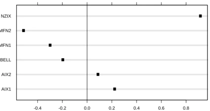
We fitted the model to the live data and to the synthetic data using bisquare, also accommodating the changing value ofmδj(ψ). Figure 5 shows dotplots of the 6 medians of the residuals for the 6 links. There is a clear link effect, mimicing the behavior Figure 4; the two links with the largest and smallest residual medians are the two with the largest and smallest median connection bit rates. The behavior of these extremes is what we would expect. For example, NZIX has the smallest median γb, so its bit rate under-predicts the utilization because a
stream at NZIX with a certainτ has more multiplexing than average than streams at other links with the sameτ, which means the favorable statistical properties push the utilization higher than expected under the model. The same plot for the synthetic streams shows the same effect.
In addition, there is another inadequacy of this first model. Becauseγb is changing, we want the model to obey
the principle of fast-forward invariance, but it does not because the estimates ofoτ andoδare not equal.
We will enlarge the bandwidth model by adding the variable log2(c). Because log2(τ) is used in the initial model, adding log2(c) is equivalent to addingγb. In doing this we want an equation that obeys fast-forward
invariance: if we hold cfixed, multiply τ by h, and divideδ by h, then we do not want a change in the QoS utilization. This is achieved by the Best-Effort Delay Model:
logit2(uijk) =o+oclog2(ci) +oτ δlog2(τiδj) +oω(−log2(−log2(ωk))) +ψijk (5)
where theψijkare error variables with mean 0 and median absolute deviationmδj(ψ). Fast-forward invariance is achieved by enteringτ andδas a product.
We fitted the enlarged of Equation 5 to the live streams and to the synthetic streams using bisquare because our exploration showed that the error distribution has longer tails than the normal; the estimation included a normalization to adjust for themδj(ψ). The bisquare estimates ofo,oc,oτ δ, andoω are
Live: ˆo=−8.933 ˆoc = 0.420 ˆoτ δ= 0.444 ˆoω= 0.893
Synthetic: oˆ=−8.227 ˆoc = 0.353 ˆoτ δ = 0.457 ˆoω = 0.952.
The two sets of estimates are very close in the sense that the fitted equations are close. The estimates ofmδj(ψ), the median absolute deviations,mˆδj(ψ), of the residuals, are
Delay: 1ms 5ms 10ms 50ms 100ms
Live: 0.211 0.312 0.372 0.406 0.484
Synthetic: 0.169 0.322 0.356 0.380 0.457
Again, the two sets of estimates are close.
It is important to consider whether the added variable cis contributing in a significant way to the variability in logit2(uijk), and does not depend fully on the single link NZIX. We used the partial standardized residual
plot in Figure 6 to explore this. The standardized residuals of regressing the logit utilization, logit2(u), on the predictor variables except log2(c), are graphed against the standardized residuals from regressinglog2(c) on the same variables. The partial regressions are fitted using the final bisquare weights from the full model fit, and the standardization is a division of the residuals by the estimatesmˆδj(ψ). Figure 6 shows thatlog2(c)has explanatory power for each link separately and not just across links. We can also see from the plot that there is a remaining small link effect, but a minor one. This is also demonstrated in Figure 7, the same plot as in Figure 5, but for the enlarged model; the horizontal scales on the two plots have been made the same to facilitate comparison. The major link effect is now no longer present in the enlarged model. The result is the same for the same visual display for the synthetic data.
7.8 Alternative Forms of the Best-Effort Bandwidth Formula
The Best-Effort Delay Formula of the Best-Effort Delay Model in Equation 5 is
logit2(uijk) =o+oclog2(ci) +oτ δlog2(τiδj) +oω(−log2(−log2(ωk))). (6)
Sinceτ =cγb, the formula can be rewritten as
logit2(u) =o+ (oc+oτ δ) log2(c) +oτ δlog2(γbδ) +oω(−log2(−log2(ω))). (7)
In this form we see the action of the amount of multiplexing of connections as measured byc, and the end-to-end connection speed as measured byγb. An increase in either results in an increase in the utilization of a link.
7.9 Modeling the Error Distribution
As we have discussed, our study of the residuals from the fit of the Best-Effort Delay Model showed that the scale of the residual error distribution increases with the delay. The study also showed thatlog2(mδ)is linearly
related tolog2(δ). From the least squares estimates for the live data, the estimate of the intercept of the regression line is−0.481, the estimate of the linear coefficient of the line is 0.166, and the estimate of the standard error is 0.189. (Results are similar for the synthetic data.)
We also found that when we normalized the residuals by the estimates mˆδj(ψ), the resulting distribution of values is very well approximated by a constant times at-distribution with 15 degrees of freedom. Because the normalized residuals have a median absolute deviation of 1 and thet15has a median absolute deviation of 0.691,
the constant is0.691−1
. We will use this modeling of the error distribution for the bandwidth prediction in Section 8.
8
Bandwidth Estimation
The Best-Effort Delay Model in Equation 5 can be used to estimate the bandwidth required to meet QoS criteria on delay for best-effort Internet traffic. We describe here a conservative procedure in the sense that the estimated bandwidth will be unlikely to be too small. In doing this we will use the coefficient estimates from the live delay data.
First, we estimate the expected logit utilization,`=logit2(u)by
ˆ
`=−8.933 + 0.420 log2(c) + 0.444 log2(τ δ) + 0.893(−log2(−log2(ω))).
On the utilization scale this is
ˆ
u= 2
ˆ
`
1 + 2ˆ`.
Next we compute a predicted median absolute deviation from the above linear regression:
ˆ
mδ(ψ) = 2−0.481+0.166 log2δ.
Lett15(p)be the quantile of probabilitypof atdistribution with 15 degrees of freedom. Then the lower limit
of a100(1−p)% tolerance interval for`is
ˆ
`(p) = ˆ`−mˆδ(ψ)t15(p)/0.691.
Forp= 0.05,t15(p) =1.75, so the lower 95% limit is
ˆ
`(0.05) = ˆ`−2.53 ˆmδ(ψ).
The lower 95% limit on the utilization scale is
ˆ
u(0.05) = 2
ˆ
`(0.05)
1 + 2`ˆ(0.05).
This process is illustrated in Figure 8. For the figure,γbwas taken to be214bits/sec/connection. On each panel,
the values ofτ andωare fixed to the values shown in the strip labels at the tops of the panels, anduˆanduˆ(0.05)
9
Other Work on Bandwidth Estimation and Comparison with the Results
Here
Bandwidth estimation has received much attention in the literature. The work focuses on queueing because the issue driving estimation is queueing. Some work is fundamentally empirical in nature in that it uses live streams as inputs to queueing simulations or synthetic streams from models that have been built with live streams, al-though theory can be invoked as well. Other work is fundamentally theoretical in nature in that the goal is to derive mathematically properties of queues, although live data are sometimes used to provide values of param-eters so that numerical results can be calculated. Most of this work uses derivations of the delay exceedance probability as a function of an input source to derive the required bandwidth for a given QoS requirement. The delay exceedance probability is equivalent to the our delay probability, where the buffer size is related to the delay by a simple multiplication of the link bandwidth. Since exact calculations of the delay probability are only feasible in special cases, these methods seek an approximate analysis, for example, using asymptotic meth-ods, stochastic bounds, or in some cases, simulations. There has been by far much more theoretical work than empirical.
The attention to the statistical properties of the traffic stream, which have an immense impact on the queueing, receives attention to varying degrees. Those who carry out empirical studies with live streams do so as a guar-antee of recreating the properties. Those who carry out studies with synthetic traffic from models must argue for the validity of the models. Much of the theoretical work takes the form of assuming certain stream properties and then, deriving the consequences, so the problem is solved for any traffic that might have these properties. Sometime, though, the problem is minimized by deriving asymptotic results under general conditions.
9.1 Empirical Study
Our study here falls in the empirical category but with substantial guidance from theory. To estimate exceedance probabilities, we run simulations of an infinite buffer, FIFO queue with fixed utilization using live packet streams or synthetic streams from the FSD model as the input source.
In a very important study it was shown that long-range dependent traffic results in much greater queue-length distributions (Erramilli, Narayan, and Willinger 1996) than Poisson traffic. This was an important result because it showed that the long-range dependence of the traffic would have a large impact on Internet engineering. In other studies, queueing simulations of both live and altered live traffic are used to study the effect of dependence properties and multiplexing on performance using the average queue length as the performance metric (Erramilli, Narayan, Neidbardt, and Saniee 2000; Cao, Cleveland, Lin, and Sun 2001; Erramilli, Narayan, Neidbardt, and Saniee 2000).
In (Mandjes and Boots 2004), queueing simulations of multiplexed on-off sources are used to study the influence of on and off time distributions on the shape of the loss curve and on performance. To improve the accuracy of the delay probabilities based on simulations, techniques such as importance sampling are also considered (Boots and Mandjes 2001).
One study (Fraleigh, Tobagi, and Diot 2003) first uses live streams, Internet backbone traffic, to validate a traffic model: an extension of Fractional Brownian Motion (FBM), a two-scale FBM process. They do not model the packet process but rather bit rates as a continuous function. Then they derive approximations of the delay exceedance probability from the model, which serves as the basis for their bandwidth estimation. Parameters in the two-scale FBM model that appear in the formula are related to the bitrate τ using the data. This is similar to our process here where we relate the stream coefficients tocandτ. They also used queueing simulations to determine delay exceedance probabilities as a method of validation. We will compare their results and ours at the end of this section.
9.2 Mathematical Theory: Effective Bandwidth
A very large number of publications have been written in an area of bandwidth estimation that is referred to as “effective bandwidth”. The effective bandwidth of an input source provides a measure of its resource usage for a given QoS requirement, which should lie somewhere between the mean rate and peak rate. LetA(t)be the total workload (e.g., bytes) generated by a source in the interval [0, t], the mathematical definition of the effective
bandwidth of the source (Kelly 1996) is
α(s, t) = 1
stlog E[e
sA(t)] 0< s, t <
∞, (8)
for some space parametersand time parameter t. For the purpose of bandwidth estimation, the appropriate choice of parameters depends on the traffic characteristics of the source, the QoS requirements, as well as the properties of the traffic with which the source is multiplexed. In the following we shall discuss the effective bandwidth approach to bandwidth estimation based on approximating the delay probability in the asymptotic regime of many sources.
Consider the delay exceedance probability for a First In First Out (FIFO) queue on a link with constant bit rate. In the asymptotic regime of many sources, we are concerned with how the delay probability decays as the size of the system increases. Suppose there are nsources and the traffic generated by the nsources are identical, independent and stationary. The number of sources, n, grows large and at the same time the resources such as the link bandwidthβ and buffer sizes scale proportionally so that the delayδstays constant. Letβ =nβ0
for someβ0, and let Qnbe the queueing delay. Under very general conditions, it can be shown that (Botvich
and Duffield 1995; Courcoubetis and Weber 1996; Simonian and Guibert 1995; Likhanov and Mazumdar 1998; Mandjes and Kim 2001)
lim n→∞−n −1 log P(Qn> δ) =I(δ, β0), (9) where I(δ, β0) = inf t>0sups (sβ0(δ+t)−stα(s, t)), (10)
and is sometimes referred to as the loss curve in the literature. Let (s∗
, t∗
) be an extremizing pair in Equa-tion (10), thenα(s∗
, t∗
)is the effective bandwidth for the single source as defined in Equation (8), andnα(s∗
, t∗
)
is the effective bandwidth for thensources. For a QoS requirement of a delayδ and a delay probabilityw, ap-proximating the delay probabilityP(Qn> δ)usingexp(−nI(δ, β0))(Equation 9), the bandwidth required for
thensources can be found by solving the following equation forβ
s∗ β(δ+t∗ )−s∗ t∗ nα(s∗ , t∗ ) =−logw. (11) This gives β= s ∗ t∗ s∗(δ+t∗)nα(s ∗ , t∗ )− logw s∗(δ+t∗), (12)
which is the effective bandwidth solution to the bandwidth estimation problem. If the delayδ → ∞, then the extremizing value oft∗
approaches to∞, and the bandwidth in Equation (12) reduces to
n lim
t∗→∞α(s ∗
, t∗
),
and we recover the classical effective bandwidth definition of a single source limt∗→∞α(s ∗
, t∗
)for the large buffer asymptotic model (Elwalid and Mitra 1993; Guerin, Ahmadi, and Naghshineh 1991; Kesidis, Walrand, and Chang 1993; Chang and Thomas 1995). If the delayδ →0, then the extremizing pairt∗
→0ands∗
t∗
→˜s
for somes˜, the bandwidth in Equation (12) reduces to
n lim t∗→∞α(˜s/t ∗ , t∗ )−logw ˜ s ,
and we recover the effective bandwidth definitionlimt∗→∞α(˜s/t ∗
, t∗
)for the buffer-less model (Hui 1988). As we can see, the effective bandwidth solution requires the evaluation of the loss curveI(δ, β0)(Equation 10).
However, explicit form of the loss curve is generally not available. One approach is to derive approximations of the loss curve under buffer asymptotic models, i.e., large buffer asymptotic model (δ → ∞) or buffer-less model (δ→0), for some classes of input source arrivals. For example, if the source arrival process is Markovian, then for someη >0andν(Botvich and Duffield 1995)
lim
δ→∞
I(δ, β0)−ηδ =ν.
If the source arrival is Fractional Brownian Motion with Hurst parameter H, then for someν > 0(Duffield 1996)
lim
δ→∞
I(δ, β0)/δ2−2H =ν.
For on-off fluid arrival process, it is shown that asδ → 0, for some constantsη(β0)andν(β0)(Mandjes and
Kim 2001),
I(δ, β0)∼η(β0) +ν(β0)
√
δ+O(δ),
and asδ→ ∞, for some constantθ(β0)(Mandjes and Boots 2002),
I(δ, β0)∼θ(β0)v(δ),
wherev(δ) =−log P(Residual On period> δ). However, it is found that bandwidth estimation based on buffer asymptotic models suffer practical problems. For the large buffer asymptotic model, the estimated bandwidth
could be overly conservative or optimistic due to the fact that it does not take into account the statistical mul-tiplexing gain (Choudhury, Lucantoni, and Whitt 1994; Knightly and Shroff 1999). For the buffer-less model, there is a significant utilization penalty in the estimated bandwidth (Knightly and Shroff 1999) since results indicate that there is a significant gain even with a small buffer (Mandjes and Kim 2001).
Another approach proposed by (Courcoubetis, Siris, and Stamoulis 1999; Courcoubetis and Siris 2001) is to numerically evaluate the loss curveI(δ, β0). First, they evaluate the effective bandwidth functionα(s, t)
(Equa-tion 8) empirically based on measurements of traffic byte counts in fixed size intervals, and then they obtain the loss curve (Equation 10) using numeric optimizing procedures with respect to the space parametersand the time parameter t. As examples, they applied this approach to estimate bandwidth where the input source is a Bellcore Ethernet WAN streams or streams of incoming IP traffic over the University of Crete’s wide area link. Their empirical approach is model free in the sense that it does not require a traffic model for the input source and all evaluations are based on traffic measurements. However, their approach is computational intensive, not only because the effective bandwidth function α(s, t) has to be evaluated for all time parameters t, but also because the minimization with respect totis non-convex (unlike the maximization in the space parameters) and thus difficult to perform numerically (Gibbens and Teh 1999; Kontovasilis, Wittevrongel, Bruneel, Houdt, and Blondia 2002).
In the effective bandwidth approach, one typically approximates the buffer exceedance probability based on its logarithmic asymptote. For example, in the asymptotic regime of many sources, using Equation (9), one can approximate
P(Qn> δ)≈exp(−nI(δ, β0)). (13)
An improved approximation can be found by incorporating a pre-factor, i.e.
P(Qn> δ)≈K(n, δ, β0) exp(−nI(δ, β0)).
Using the Bahadur-Rao theorem, such approximation has been obtained for the delay exceedance probability in the infinite buffer case as well as the cell loss ratio in the finite buffer case that has the same logarithmic asymptote but a different pre-factor (Likhanov and Mazumdar 1998).