A Comparison of Overlay Routing and
Multihoming Route Control
Aditya Akella
Jeffrey Pang
Bruce Maggs
†Srinivasan Seshan
Carnegie Mellon University
{aditya, jeffpang,srini+, bmm}@cs.cmu.edu
Anees Shaikh
IBM T.J. Watson Research Center aashaikh@watson.ibm.com
ABSTRACT
The limitations of BGP routing in the Internet are often blamed for poor end-to-end performance and prolonged connectivity interrup-tions. Recent work advocates using overlays to effectively bypass BGP’s path selection in order to improve performance and fault tolerance. In this paper, we explore the possibility that intelligent control of BGP routes, coupled with ISP multihoming, can provide competitive end-to-end performance and reliability. Using exten-sive measurements of paths between nodes in a large content distri-bution network, we compare the relative benefits of overlay routing and multihoming route control in terms of round-trip latency, TCP connection throughput, and path availability. We observe that the performance achieved by route control together with multihoming to three ISPs (3-multihoming), is within 5-15% of overlay rout-ing employed in conjunction 3-multihomrout-ing, in terms of both end-to-end RTT and throughput. We also show that while multihom-ing cannot offer the nearly perfect resilience of overlays, it can eliminate almost all failures experienced by a singly-homed end-network. Our results demonstrate that, by leveraging the capabil-ity of multihoming route control, it is not necessary to circumvent BGP routing to extract good wide-area performance and availabil-ity from the existing routing system.
Categories and Subject Descriptors
C.2 [Computer Systems Organization]: Computer-Communication Networks; C.2.1 [Computer-Communication Networks]: Net-work Architecture and Design
General Terms
Measurement, Performance, Reliability
Keywords
multihoming, route control, overlay routing
†
Bruce Maggs is also with Akamai Technologies.
This work was supported by the Army Research Office under grant number DAAD19-02-1-0389. Additional support was provided by IBM.
Permission to make digital or hard copies of all or part of this work for personal or classroom use is granted without fee provided that copies are not made or distributed for profit or commercial advantage and that copies bear this notice and the full citation on the first page. To copy otherwise, to republish, to post on servers or to redistribute to lists, requires prior specific permission and/or a fee.
SIGCOMM’04, August 30–September 3, 2004, Portland, OR.
Copyright 2004 ACM 1-58113-862-8/04/0008 ...$5.00.
1.
INTRODUCTION
The limitations of conventional Internet routing based on the Border Gateway Protocol (BGP) are often held responsible for fail-ures and poor performance of end-to-end transfers. A number of studies have shown that the underlying connectivity of the Internet is capable of providing much greater performance and resilience than end-points currently receive. Such studies, exemplified by Detour [25, 26] and RON [6], demonstrate that using overlay rout-ing to bypass BGP’s policy-driven routrout-ing enables quicker reaction to failures and improved end-to-end performance. In this paper, we question whether overlay routing is required to make the most of the underlying connectivity, or whether better selection of BGP routes at an end-point is sufficient.
There are two key factors contributing to the differences between overlay routing and BGP-based routing that have not been carefully evaluated in past work: the number of routing choices available to each system and the policies used to select among these routes.
Route Availability. By allowing sources to specify a set of
inter-mediate hops, overlay routing allows end-points nearly arbitrary control over the wide-area path that packets take. On the other hand, BGP only allows a network to announce routes that it ac-tually uses. Thus, to reach a given destination, an end-point has access to only a single path from each Internet Service Provider (ISP) to which it is attached [30]. As a result, an end-point’s ability to control routing is tightly linked to the number of ISP connections it has.
Past studies showing the relative benefits of overlay routing draw conclusions based on the highly restrictive case wherein paths from just a single ISP are available [6, 25]. In contrast, in this paper, we carefully consider the degree of ISP multihoming at the end-point, and whether it provides sufficient (BGP) route choices for the end-point to obtain the same performance as when employing an overlay network.
Route Selection. In addition to having a greater selection of routes
to choose from than BGP, overlay routing systems use much more sophisticated policies in choosing the route for any particular trans-fer. Overlays choose routes that optimize end-to-end performance metrics, such as latency. On the other hand, BGP employs much simpler heuristics to select routes, such as minimizing AS hop count or cost. However, this route selection policy is not intrinsic to BGP-based routing – given an adequate selection of BGP routes, end-points can choose the one that results in the best performance, availability, or cost. Several commercial vendors already enable such route control or selection (e.g., [19, 21, 24]).
In this paper, we compare overlays with end-point based mech-anisms that use this form of “intelligent” route control of the BGP paths provided by their ISPs. Hereafter, we refer to this as multi-homing route control or simply, route control. Notice that we do
not assume any changes or improvements to the underlying BGP protocol. Multihoming route control simply allows a multihomed end-network to intelligently schedule its transfers over multiple ISP links in order to optimize performance, availability, cost or a com-bination of these metrics.
Our goal is to answer the question: How much benefit does over-lay routing provide over BGP, when multihoming and route con-trol are considered? If the benefit is small, then BGP path selec-tion is not as inferior as it is held to be, and good end-to-end per-formance and reliability are achievable even when operating com-pletely within standard Internet routing. On the other hand, if over-lays yield significantly better performance and reliability character-istics, we have further confirmation of the claim that BGP is fun-damentally limited. Then, it is crucial to develop alternate bypass architectures such as overlay routing.
Using extensive active downloads and traceroutes between 68 servers belonging to a large content distribution network (CDN), we compare multihoming route control and overlay routing in terms of three key metrics: round-trip delay, throughput, and availabil-ity. Our results suggest that when route control is employed along with multihoming, it can offer performance similar to overlays in terms of trip delay and throughput. On average, the round-trip times achieved by the best BGP paths (selected by an ideal route control mechanism using 3 ISPs) are within 5–15% of the best overlay paths (selected by an ideal overlay routing scheme also multihomed to 3 ISPs). Similarly, the throughput on the best overlay paths is only 1–10% better than the best BGP paths. We also show that the marginal difference in the RTT performance can be attributed mainly to overlay routing’s ability to select shorter paths, and that this difference can be reduced further if ISPs im-plement cooperative peering policies. In comparing the end-to-end path availability provided by either approach, we show that multi-homing route control, like overlay routing, is able to significantly improve the availability of end-to-end paths.
This paper is structured as follows. In Section 2, we describe past work that demonstrates limitations in the current routing sys-tem, including work on overlay routing and ISP multihoming. Sec-tion 3 provides an overview of our approach. SecSec-tion 4 gives de-tails of our measurement testbed. In Section 5, we analyze the RTT and throughput performance differences between route control and overlay routing and consider some possible reasons for the differ-ences. In Section 6, we contrast the end-to-end availability offered by the two schemes. Section 7 discusses the implications of our results and presents some limitations of our approach. Finally, Sec-tion 8 summarizes the contribuSec-tions of the paper.
2.
RELATED WORK
Past studies have identified and analyzed several shortcomings in the design and operation of BGP, including route convergence behavior [16, 17] and “inflation” of end-to-end paths due to BGP policies [28, 32]. Particularly relevant to our study are proposals for overlay systems to bypass BGP routing to improve performance and fault tolerance, such as Detour [25] and RON [6].
In the Detour work, Savage et al. [25] study the inefficiencies of wide-area routing on end-to-end performance in terms of round-trip time, loss rate, and throughput. Using observations drawn from active measurements between public traceroute server nodes, they compare the performance on default Internet (BGP) paths with the potential performance from using alternate paths. This work shows that for a large fraction of default paths measured, there are alter-nate indirect paths offering much better performance.
Andersen et al. propose Resilient Overlay Networks (RONs) to address the problems with BGP’s fault recovery times, which have
been shown to be on order of tens of minutes in some cases [6]. RON nodes regularly monitor the quality and availability of paths to each other, and use this information to dynamically select di-rect or indidi-rect end-to-end paths. RON mechanisms are shown to significantly improve the availability and performance of end-to-end paths between the overlay nodes. The premise of the Detour and RON studies is that BGP-based route selection is fundamen-tally limited in its ability to improve performance and react quickly to path failures. Both Detour and RON compare the performance and resilience of overlay paths against default paths via a single provider. Overlays offer a greater choice of end-to-end routes, as well as greater flexibility in controlling the route selection. In con-trast, we explore the effectiveness of empowering BGP-based route selection with intelligent route control at multihomed end-networks in improving end-to-end availability and performance relative to overlay routing.
Also, several past studies have focused on “performance-aware” routing, albeit not from an end-to-end perspective. Proposals have been made for load sensitive routing within ISPs (see [27], for ex-ample) and, intra- and inter-domain traffic engineering [10, 23, 15]. However, the focus of these studies is on balancing the utilization on ISP links and not necessarily on end-to-end performance. More directly related to our work is a recent study on the potential of multihoming route control to improve end-to-end performance and resilience, relative to using paths through a single ISP [3]. Finally, a number of vendors have recently developed intelligent routing appliances that monitor availability and performance over multi-ple ISP links, and automatically switch traffic to the best provider. These products facilitate very fine-grained selection of end-to-end multihoming routes (e.g., [8, 19, 21, 24]).
3.
COMPARING BGP PATHS WITH
OVER-LAY ROUTING
Our objective is to understand whether the modest flexibility of multihoming, coupled with route control, is able to offer end-to-end performance and resilience similar to overlay routing. In order to answer this question, we evaluate an idealized form of multihoming route control where the end-network has instantaneous knowledge about the performance and availability of routes via each of its ISPs for any transfer. We also assume that the end-network can switch between candidate paths to any destination as often as desired. Fi-nally, we assume that the end-network can easily control the ISP link traversed by packets destined for its network (referred to as “inbound control”).
In a real implementation of multihoming route control, however, there are practical limitations on the ability of an end-network to track ISP performance, on the rate at which it can switch paths, and on the extent of control over incoming packets. However, recent work [4] shows that simple active and passive measurement-based schemes can be employed to obtain near-optimal availability, and RTT performance that is within 5-10% of the optimal, in practical multihomed environments. Also, simple NAT-based techniques can be employed to achieve inbound route control [4].
To ensure a fair comparison, we study a similarly agile form of overlay routing where the end-point has timely and accurate knowl-edge of the best performing, or most available, end-to-end overlay paths. Frequent active probing of each overlay link, makes it pos-sible to select and switch to the best overlay path at almost any instant when the size of the overlay network is small (∼50 nodes)1. We compare overlay routing and route control with respect to the degree of flexibility available at the end-network. In general,
1
this flexibility is represented byk, the number of ISPs available to either technique at the end-network. In the case of route control, we considerk-multihoming, where we evaluate the performance and reliability of end-to-end candidate paths induced by a combi-nation ofkISPs. For overlay routing, we introduce the notion of k-overlays, wherekis the number of providers available to an end-point for any end-to-end overlay path. In other words, this is simply overlay routing in the presence ofkISP connections.
When comparingk-multihoming withk-overlays, we report re-sults based on the combination ofkISPs that gives the best per-formance (RTT or throughput) across all destinations. In prac-tice an end-network cannot purchase connectivity from all available providers, or easily know which combination of ISPs will provide the best performance. Rather, our results demonstrate how much flexibility is necessary, in terms of the number of ISP connections, and the maximum benefit afforded by this flexibility.
end-network ISP BGP direct paths 3-multihomed network route controller
(a) single ISP, BGP routing (b) multihoming with 3 ISPs
(1-multihoming) (3-multihoming) overlay paths overlay paths 3-multihomed with overlay routing
(c) single ISP, overlay routing (d) overlay routing with
(1-overlay) multihoming (3-overlay)
Figure 1: Routing configurations: Figures (a) and (b) show 1-multihoming and 3-1-multihoming, respectively. Corresponding overlay configurations are shown in (c) and (d), respectively.
Figure 1 illustrates some possible route control and overlay con-figurations. For example, (a) shows the case of conventional BGP routing with a single default provider (i.e., 1-multihoming). Fig-ure 1(b) depicts end-point route control with three ISPs (i.e., 3-multihoming). Overlay routing with a single first-hop provider (i.e., 1-overlay) is shown in Figure 1(c), and Figure 1(d) shows the case of additional first-hop flexibility in a 3-overlay routing configura-tion.
We seek to answer the following key questions:
1. On what fraction of end-to-end paths does overlay routing outperform multihoming route control in terms of RTT and throughput? In these cases, what is the extent of the perfor-mance difference?
2. What are the reasons for the performance differences? For
example, must overlay paths violate inter-domain routing poli-cies to achieve good end-to-end performance?
3. Does route control, when supplied with sufficient flexibility in the number of ISPs, achieve path availability rates that are comparable with overlay routing?
4.
MEASUREMENT TESTBED
Addressing the questions posed in Section 3 from the perspective of an end-network requires an infrastructure which provides access to a number of BGP path choices via multihomed connectivity, and the ability to select among those paths at a fine granularity. We also require an overlay network with a reasonably wide deployment to provide a good choice of arbitrary wide-area end-to-end paths which could potentially bypass BGP policies.
We address both requirements with a single measurement testbed consisting of nodes belonging to the server infrastructure of the Akamai CDN. Following a similar methodology to that described in [3], we emulate a multihoming scenario by selecting a few nodes in a metropolitan area, each singly-homed to a different ISP, and use them collectively as a stand-in for a multihomed network. Rela-tive to previous overlay routing studies [25, 6], our testbed is larger with 68 nodes. Also, since the nodes are all connected to com-mercial ISPs, they avoid paths that traverse Internet2, which may introduce unwanted bias due their higher bandwidth and lower like-lihood of queuing, compared to typical Internet paths. Our mea-surements are confined to nodes located in the U.S., though we do sample paths traversing ISPs at all levels of the Internet hierarchy from vantage points in many major U.S. metropolitan areas.
The 68 nodes in our testbed span 17 U.S. cities, averaging about four nodes per city, connected to commercial ISPs of various sizes. The nodes are chosen to avoid multiple servers attached to the same provider in a given city. The list of cities and the tiers of the cor-responding ISPs are shown in Figure 2(a). The tiers of the ISPs are derived from the work in [31]. The geographic distribution of the testbed nodes is illustrated in Figure 2(b). We emulate multi-homed networks in 9 of the 17 metropolitan areas where there are at least 3 providers – Atlanta, Bay Area, Boston, Chicago, Dallas, Los Angeles, New York, Seattle and Washington D.C.
City Providers/tier 1 2 3 4 5 Atlanta, GA 2 0 1 1 0 Bay Area, CA 5 0 3 1 2 Boston, MA 1 0 1 0 1 Chicago, IL 6 1 0 1 0 Columbus, OH 0 1 0 1 0 Dallas, TX 3 0 0 1 0 Denver, CO 1 0 0 0 0 Des Moines, IO 0 1 0 0 0 Houston, TX 1 1 0 0 0 Los Angeles, CA 3 0 3 0 0 Miami, FL 1 0 0 0 0 Minneapolis, MN 0 0 1 0 0 New York, NY 3 2 2 1 0 Seattle, WA 2 0 2 1 1 St Louis, MO 1 0 0 0 0 Tampa, FL 0 1 0 0 0 Washington DC 3 0 3 0 2 # # # # # # # # # # # # # # # # #
(a) Testbed ISPs (b) Node locations
Figure 2: Testbed details: The cities and distribution of ISP tiers in our measurement testbed are listed in (a). The geo-graphic location is shown in (b). The area of each dot is pro-portional to the number of nodes in the region.
5.
LATENCY AND THROUGHPUT
PERFORMANCE
We now present our results on the relative latency and through-put performance benefits of multihoming route control compared with overlay routing. We first describe our data collection method-ology (Section 5.1) and evaluation metrics (Section 5.2). Then, we present the key results in the following order. First we com-pare 1-multihoming against 1-overlays along the same lines as the analysis in [25] (Section 5.3). Next, we compare the benefits of us-ingk-multihoming andk-overlay routing, relative to using default paths through a single provider (Section 5.4). Then, we compare k-multihoming against 1-overlay routing, fork≥1(Section 5.5). Here, we wish to quantify the benefit to end-systems of greater flexibility in the choice of BGP routes via multihoming, relative to the power of 1-overlays. Next, we contrastk-multihoming against k-overlay routing to understand the additional benefits gained by allowing end-systems almost arbitrary control on end-to-end paths, relative to multihoming (Section 5.6). Finally, we examine some of the underlying reasons for the performance differences (Sec-tions 5.7 and 5.8).
5.1
Data Collection
Our comparison of overlays and multihoming is based on obser-vations drawn from two data sets collected on our testbed. The first data set consists of active HTTP downloads of small objects (10 KB) to measure the turnaround times between the pairs of nodes. The turnaround time is the time between the transfer of the last byte of the HTTP request and the receipt of the first byte of the response, and provides an estimate of the round-trip time. Hereafter, we will use the terms turnaround time and round-trip time interchangeably. Every 6 minutes, turnaround time samples are collected between all node-pairs (including those within the same city).
The second data set contains “throughput” measurements from active downloads of 1 MB objects between the same set of pairs. These downloads occur every 30 minutes between all node-pairs. Here, throughput is simply the size of the transfer (1 MB) divided by the time between the receipt of the first and last bytes of the response data from the server (source). As we discuss in Section 5.2, this may not reflect the steady-state TCP throughput along the path.
Since our testbed nodes are part of a production infrastructure, we limit the frequencies at which all-pairs measurements are col-lected as described above. To ensure that all active probes between pairs of nodes observe similar network conditions, we scheduled them to occur within a 30 second interval for the round-trip time data set, and within a 2 minute interval for the throughput data set. For the latter, we also ensure that an individual node is involved in at most one transfer at any time so that our probes do not contend for bandwidth at the source or destination network. The transfers may interfere elsewhere in the Internet, however. Also, since our testbed nodes are all located in the U.S., the routes we probe, and consequently, our observations, are U.S.-centric.
The round-trip time data set was collected from Thursday, De-cember 4th, 2003 through Wednesday, DeDe-cember 10th, 2003. The throughput measurements were collected between Thursday, May 6th, 2004 and Tuesday, May 11th, 2004 (both days inclusive).
5.2
Performance Metrics
We compare overlay routing and multihoming according to two metrics derived from the data above: round-trip time (RTT) and throughput. In the RTT data set, for each 6 minute measurement interval, we build a weighted graph over all the 68 nodes where the edge weights are the RTTs measured between the corresponding
node-pairs. We then use Floyd’s algorithm to compute the shortest paths between all node-pairs. We estimate the RTT performance from usingk-multihoming to a given destination by computing the minimum of the RTT estimates along the direct paths from thek ISPs in a city to the destination node (i.e., the RTT measurements between the Akamai CDN nodes representing thekISPs and the destination node). To estimate the performance ofk-overlay rout-ing, we compute the shortest paths from thekISPs to the destina-tion node and choose the minimum of the RTTs of these paths.
Note that we do not prune the direct overlay edge in the graph before performing the shortest path computation. As a result, the shortest overlay path between two nodes could be a direct path (i.e., chosen by BGP). Hence our comparison is not limited to direct versus indirect paths, but is rather between direct and overlay paths. In contrast, the comparison in [25] is between the direct path and the best indirect path.
For throughput, we similarly construct a weighted, directed graph between all overlay nodes every 30 minutes (i.e., our 1 MB ob-ject download frequency). The edge weights are the throughputs of the 1 MB transfers (where throughput is computed as described in Section 5.1). We compute the throughput performance of k -multihoming andk-overlay routing similar to the RTT performance computation above. Notice, however, that computing the overlay throughput performance is non-trivial and is complicated by the problem of estimating the end-to-end throughput for a 1 MB TCP transfer on indirect overlay paths.
Our approach here is to use round-trip time and throughput mea-surements on individual overlay hops to first compute the under-lying loss rates. Since it is likely that the paths we measure do not observe any loss, thus causing the transfers to likely remain in their slow-start phases, we use the small connection latency model developed in [7]. The typical MSS in our 1MB transfers is 1460 bytes. Also, the initial congestion window size is 2 segments and there is no initial 200ms delayed ACK timeout on the first transfer. In the throughput data set, we measure a mean loss rate of 1.2% and median, 90th, 95th and 99th percentile loss rates of 0.004%, 0.5%, 1% and 40% across all paths measured, respectively.
We can then use the sum of round-trip times and a combination of loss rates on the individual hops as the end-to-end round-trip time and loss rate estimates, respectively, and employ the model in [7] to compute the end-to-end overlay throughput for the 1 MB transfers. To combine loss rates on individual links, we follow the same approach as that described in [25]. We consider two possible combination functions. The first, called optimistic, uses the maxi-mum observed loss on any individual overlay hop along an overlay path as an estimate of the end-to-end overlay loss rate. This as-sumes that the TCP sender is primarily responsible for the observed losses. In the pessimistic combination, we compute the end-to-end loss rate as the sum of individual overlay hop loss rates, assuming the losses on each link to be due to independent background traf-fic in the network2. Due to the complexity of computing arbitrary length throughput-maximizing overlay paths, we only consider in-direct paths comprised of at most two overlay hops in our through-put comparison.
5.3
1-Multihoming versus 1-Overlays
First, we compare the performance of overlay routing against de-fault routes via a single ISP (i.e., 1-overlay against 1-multihoming), along the same lines as [25]. Note that, in the case of 1-overlays, the overlay path from a source node may traverse through any
in-2
The end-to-end loss rate over two overlay links with independent loss rates ofp1andp2is1−(1−p1)(1−p2) =p1+p2−p1p2.
termediate node, including nodes located in the same city as the source. City 1-multihoming/ 1-overlay Atlanta 1.35 Bay Area 1.20 Boston 1.28 Chicago 1.29 Dallas 1.32 Los Angeles 1.22 New York 1.29 Seattle 1.71 Wash D.C. 1.30 Average 1.33 0 0.2 0.4 0.6 0.8 1 1 2 3 4 5 6 7
Fraction of overlay paths with < x hops
Number of overlay hops Atlanta Bay Area Boston Chicago Dallas Los Angeles New York Seattle Washington D C
(a) 1-multihoming RTT (b) 1-overlay path length relative to 1-overlays
Figure 3: Round-trip time performance: Average RTT perfor-mance of 1-multihoming relative to 1-overlay routing is tabu-lated in (a) for various cities. The graph in (b) shows the dis-tribution of the number of overlay hops in the best 1-overlay paths, which could be the direct path (i.e., 1 overlay hop).
Round-trip time performance. Figure 3(a) shows the RTT
per-formance of 1-multihoming relative to 1-overlay routing. Here, the performance metric (y-axis) reflects the relative RTT from 1-multihoming versus the RTT when using 1-overlays, averaged over all samples to all destinations. The difference between this metric and 1 represents the relative advantage of 1-overlay routing over 1-multihoming. Notice also that since the best overlay path could be the direct BGP path, the performance from overlays is at least as good as that from the direct BGP path. We see from the ta-ble that overlay routing can improve RTTs between 20% and 70% compared to using direct BGP routes over a single ISP. The average improvement is about 33%. The observations in [25] are similar.
We show the distribution of overlay path lengths in Figure 3(b), where the direct (BGP) path corresponds to a single overlay hop. Notice that in most cities, the best overlay path is only one or two hops in more than 90% of the measurements. That is, the major-ity of the RTT performance gains in overlay networks are realized without requiring more than a single intermediate hop. Also, on an average, the best path from 1-overlays coincides with the direct BGP path in about 54% of the measurements (average y-axis value at x=1 across all cities).
Throughput performance. In Table 1, we show the throughput
performance of 1-overlays relative to 1-multihoming for both the pessimistic and the optimistic estimates. 1-overlays achieve 6– 20% higher throughput than 1-multihoming, according to the pes-simistic estimate. According to the optimistic throughput estimate, 1-overlays achieve 10–25% better throughput. In Table 1, we also show the fraction of times an indirect overlay path obtains better throughput than the direct path, for either throughput estimation function. Under the pessimistic throughput estimate, on average, 1-overlay routing benefits from employing an indirect path in about 17% of the cases. Under the optimistic estimate, this fraction is 23%.
Summary. 1-Overlays offer significantly better round-trip time
performance than 1-multihoming (33% on average). The through-put benefits are lower, but still significant (15% on average). Also, in a large fraction of the measurements, indirect 1-overlay paths offer better RTT performance than direct 1-multihoming paths.
City Pessimistic estimate Optimistic estimate
Throughput metric Fraction of Throughput metric Fraction of indirect paths indirect paths
Atlanta 1.14 17% 1.17 21% Bay Area 1.06 11% 1.10 22% Boston 1.19 22% 1.24 26% Chicago 1.12 13% 1.15 18% Dallas 1.16 18% 1.18 22% Los Angeles 1.18 15% 1.21 17% New York 1.20 14% 1.25 26% Seattle 1.18 28% 1.25 35% Wash D.C. 1.09 13% 1.13 18% Average 1.15 17% 1.19 23%
Table 1: Throughput performance: This table shows the 1 MB TCP transfer performance of overlay routing relative to 1-multihoming (for both estimation functions). Also shown is the fraction of measurements in which 1-overlay routing selects an indirect path in each city.
5.4
1-Multihoming versus
k-Multihoming and
k
-Overlays
In this section we compare the flexibility offered by multihom-ing route control at an end point in isolation, and in combination with overlay routing, against using default routes via a single ISP (i.e.,k-multihoming andk-overlays against 1-multihoming). The main purpose of these comparisons is to establish a baseline for the upcoming head-to-head comparisons betweenk-multihoming and k-overlay routing in Sections 5.5 and 5.6.
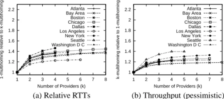
1 1.2 1.4 1.6 1.8 2 2.2 1 2 3 4 5 6 7 8
1-multihoming relative to k-multihoming
Number of Providers (k) Atlanta Bay Area Boston Chicago Dallas Los Angeles New York Seattle Washington D C 1 1.2 1.4 1.6 1.8 2 2.2 1 2 3 4 5 6 7 8
k-multihoming relative to 1-multihoming
Number of Providers (k) Atlanta Bay Area Boston Chicago Dallas Los Angeles New York Seattle Washington D C
(a) Relative RTTs (b) Throughput (pessimistic)
Figure 4: Benefits of k-multihoming: The RTT of
1-multihoming relative to k-multihoming is shown in (a) and
throughput (pessimistic estimate) ofk-multihoming relative to
1-multihoming is shown in (b).
1-Multihoming versus k-multihoming. Figure 4(a) shows the
RTT performance of 1-multihoming relative to the RTT perfor-mance fromk-multihoming averaged across all samples to all des-tinations (y-axis), as a function of the number of providers,k (x-axis). Note that the difference between the performance metric on the y-axis and 1 indicates the relative advantage ofk-multihoming over 1-multihoming. The RTT benefit from multihoming is about 15–30% fork = 2 and about 20–40% fork = 3across all the cities. Also, beyondk= 3or4the marginal improvement in the RTT performance from multihoming is negligible. The observa-tions made by Akella et al. in [3] are similar.
Figure 4(b) similarly shows the throughput performance ofk -multihoming relative to the throughput from 1--multihoming, ac-cording to the pessimistic estimate. The results for the optimistic estimate are similar and are omitted for brevity. Again,k-multihoming, fork= 3, achieves 15–25% better throughput than 1-multihoming
and the marginal improvement in the throughput performance is negligible beyondk= 3. 1 1.2 1.4 1.6 1.8 2 2.2 1 2 3 4 5 6 7 8
1-multihoming relative to k-overlays
Number of Providers (k) Atlanta Bay Area Boston Chicago Dallas Los Angeles New York Seattle Washington D C 1 1.2 1.4 1.6 1.8 2 2.2 1 2 3 4 5 6 7 8
k-overlays relative to 1-multihoming
Number of Providers (k) Atlanta Bay Area Boston Chicago Dallas Los Angeles New York Seattle Washington D C
(a) Relative RTTs (b) Throughput (pessimistic)
Figure 5: Benefits ofk-overlays: The RTT of 1-multihoming
relative to k-overlays is shown in (a) and throughput
(pes-simistic estimate) of k-overlays relative to 1-multihoming is
shown in (b).
1-Multihoming versusk-overlays. In Figure 5(a), we show the
RTT performance of 1-multihoming relative tok-overlays as a func-tion ofk. Notice thatk-overlay routing achieves 25–80% better RTT performance than 1-multihoming, fork= 3. Notice also, that the RTT performance fromk-overlay routing, fork≥3, is about 5–20% better than that from 1-overlay routing. Figure 5(b) simi-larly compares the throughput performance ofk-overlays relative to 1-multihoming, for the pessimistic estimate. Again,3-overlay routing, for example, is 20–55% better than 1-multihoming and about 10–25% better than 1-overlay routing. The benefit beyond k = 3 is marginal across most cities, for both RTT as well as throughput.
Summary. Bothk-multihoming andk-overlay routing offer
sig-nificantly better performance than 1-multihoming, in terms of both RTT and throughput. In addition,k-overlay routing, fork ≥ 3
achieves significantly better performance compared to 1-overlay routing (5–20% better according to RTT and 10–25% better ac-cording to throughput).
5.5
k-Multihoming versus 1-Overlays
So far, we have evaluated multihoming route control (i.e., k -multihoming fork ≥2) and overlay routing in isolation of each other. In what follows, we provide a head-to-head comparison of the two systems. First, in this section, we allow end-points the flexibility of multihoming route control and compare the resulting performance against 1-overlays.
In Figure 6, we plot the performance ofk-multihoming relative to 1-overlay routing. Here, we compute the average ratio of the best RTT or throughput to a particular destination, as achieved by either technique. The average is taken over paths from each city to destinations in other cities, and over time instants for which we have a valid measurement over all ISPs in the city.3 We also note that in all but three cities, the best 3-multihoming providers accord-ing to RTT were the same as the best 3 accordaccord-ing to throughput; in the three cities where this did not hold, the third and fourth best providers were simply switched and the difference in throughput performance between them was less than 3%.
3
Across all cities, an average of 10% of the time instants did not have a valid measurement across all providers; nearly all of these cases were due to limitations in our data collection infrastructure, and not failed download attempts.
0.8 0.9 1 1.1 1.2 1.3 1.4 1.5 1.6 1.7 1 2 3 4 5 6 7 8
k-multihoming relative to 1-overlay
Number of providers (k) Atlanta Bay Area Boston Chicago Dallas Los Angeles New York Seattle Washington D C 0.8 0.9 1 1.1 1.2 1.3 1.4 1.5 1.6 1.7 1 2 3 4 5 6 7 8
1-overlay relative to k-multihoming
Number of providers (k) Atlanta Bay Area Boston Chicago Dallas Los Angeles New York Seattle Washington D C
(a) Relative RTTs (b) Throughput (pessimistic)
Figure 6: Multihoming versus 1-overlays: The RTT of k
-multihoming relative to 1-overlays is shown in (a) and
through-put (pessimistic) of 1-overlays relative tok-multihoming in (b).
The comparison according to RTT is shown in Figure 6(a). The relative performance advantage of 1-overlays is less than 5% for k= 3in nearly all cities. In fact, in some cities, e.g., Bay Area and Chicago, 3-multihoming is marginally better than overlay routing. As the number of ISPs is increased, multihoming is able to provide shorter round-trip times than overlays in many cities (with the ex-ception of Seattle). Figure 6(b) shows relative benefits according to the pessimistic throughput estimate. Here, multihoming fork≥3
actually provides 2–12% better throughput than 1-overlays across all cities. The results are similar for the optimistic computation and are omitted for brevity.
Summary. The performance advantages of 1-overlays are vastly
reduced (or eliminated) when the end-point is allowed greater flex-ibility in the choice of BGP paths via multihoming route control.
5.6
k-Multihoming versus
k-Overlays
In the previous section, we evaluated 1-overlay routing, where all overlay paths start from a single ISP in the source city. In this section, we allow overlays additional flexibility by permitting them to initially route through more of the available ISPs in each source city. Specifically, we compare the performance benefits of k-multihoming againstk-overlay routing.
In the case ofk-overlays, the overlay path originating from a source node may traverse any intermediate nodes, including those located in the same city as the source. Notice that the performance from k-overlays is at least as good as that from k-multihoming (since we allow overlays to take the direct path). The question, then, is how much more advantage do overlays provide if multi-homing is already employed by the source.
Round-trip time performance. Figure 7(a) shows the
improve-ment in RTT fork-multihoming relative tok-overlays, for various values ofk. We see that on average, fork = 3, overlays provide 5–15% better RTT performance than the best multihoming solu-tion in most of the cities in our study. In a few cities the benefit is greater (e.g. Seattle and Bay Area). The performance gap between multihoming and overlays is less significant fork≥4.
Figure 7(b) shows the distribution of the number of overlay hops in the paths selected by 3-overlay routing optimized for RTT. The best overlay path coincides with the best 3-multihoming BGP path in 64% of the cases, on average across all cities (Seattle and the Bay area are exceptions). Recall that the corresponding fraction for 1-overlay routing in Figure 3(b) was 54%. With more ISPs to links to choose from, overlay routing selects a higher fraction of direct BGP paths, as opposed to choosing from the greater number of indirect paths also afforded by multihoming.
1 1.1 1.2 1.3 1.4 1.5 1.6 1.7 1 2 3 4 5 6 7 8
k-multihoming relative to k-overlay
Number of Providers (k) Atlanta Bay Area Boston Chicago Dallas Los Angeles New York Seattle Washington D C 0 0.2 0.4 0.6 0.8 1 1 2 3 4 5 6 7
Fraction of overlay paths with < x hops
Number of overlay hops Atlanta Bay Area Boston Chicago Dallas Los Angeles New York Seattle Washington D C
(a) Relative RTTs (b) 3-Overlay path length
Figure 7: Round-trip time improvement: Round-trip time
fromk-multihoming relative to k-overlay routing, as a
func-tion ofk, is shown in (a). In (b), we show the distribution of the
number of overlay hops in the bestk-overlay paths, fork=3.
1 1.1 1.2 1.3 1.4 1.5 1.6 1.7 1 2 3 4 5 6 7 8
k-overlay relative to k-multihoming
Number of providers (k) Atlanta Bay Area Boston Chicago Dallas Los Angeles New York Seattle Washington D C City Fraction of indirect paths Atlanta 5% Bay Area 1% Boston 13% Chicago 3% Dallas 8% Los Angeles 4% New York 8% Seattle 31% Wash D.C. 2% Average 8%
(a) Throughput improvement (b) Fraction of indirect (pessimistic estimate) paths in 3-overlay routing
Figure 8: Throughput improvement: Throughput
perfor-mance ofk-multihoming relative tok-overlays for various cities
is shown in (a). The table in (b) shows the fraction of
measure-ments on whichk-overlay routing selected an indirect
end-to-end path, for the case ofk= 3.
Throughput performance. Figure 8(a) shows the throughput
per-formance ofk-multihoming relative tok-overlays using the pes-simistic throughput estimation function. From this figure, we see that multihoming achieves throughput performance within 1–10% of overlays, fork = 3. The performance improves up tok = 3
or k = 4. In all the cities, the throughput performance of 4 -multihoming is within 3% of overlay routing. In Figure 8(b), we also show the fraction of measurements where an indirect 3-overlay path offers better performance than the direct 3-multihoming path, for the pessimistic throughput estimate. On average, this fraction is about 8%. Notice that this is again lower than the corresponding percentage for 1-overlays from Table 1 (≈17%).
Summary. When employed in conjunction with multihoming,
over-lay routing offers marginal benefits over employing multihoming alone. For example, multiple ISPs allows overlay routing to achieve only a 5–15% RTT improvement over multihoming route control (fork = 3), and 1–10% improvement in throughput. In addition, k-overlay routing selects a larger fraction of direct BGP-based end-to-end paths, compared to 1-overlay routing.
5.7
Unrolling the Averages
So far, we presented averages of the performance differences for various forms of overlay routing and multihoming route control. In this section, focusing on 3-overlays and 3-multihoming, we present
the underlying distributions in the performance differences along the paths we measure. Our goal in this section is to understand if the averages are particularly skewed by: (1) certain destinations, for each source city or (2) a few measurement samples on which overlays offer significantly better performance than multihoming or (3) by time-of-day or day-of-week effects.
0 0.2 0.4 0.6 0.8 1 0 5 10 15 20 25
Frac. of destinations with mean diff < x
Difference in turnaround times (ms) Atlanta Bay Area Boston Chicago Dallas Los Angeles New York Seattle Washington D C 0 0.2 0.4 0.6 0.8 1 0 1 2 3 4 5 6 7 8
Frac. of destinations with diff < x
Difference in throughputs (Mbps) Atlanta Bay Area Boston Chicago Dallas Los Angeles New York Seattle Washington D C
(a) Mean difference in (b) Mean difference in round-trip times throughputs (pessimistic)
Figure 9: Performance per destination: Figure (a) is a CDF of the mean difference in RTTs along the best overlay path and the best direct path, across paths measured from each city. Similarly, Figure (b) plots the CDF of the mean difference in throughputs (pessimistic estimate).
Performance per destination. In Figure 9(a), for each city, we
show the distribution of the average difference in RTT between the best3-multihoming path and the best 3-overlay path to each desti-nation (i.e., each point represents one destidesti-nation). In most cities, the average RTT differences across 80% of the destinations are less than 10ms. Notice that in most cities (except Seattle), the differ-ence is greater than 15ms for less than 5% of the destinations.
In Figure 9(b), we consider the distribution of the average through-put difference of the best3-multihoming path and the best3-overlay path for the pessimistic estimate of throughput. We see the through-put difference is less than 1 Mbps for 60–99% of the destinations. We also note that, for 1–5% of the destinations, the difference is in excess of 4 Mbps. Recall from Figure 8, however, that these differences result in an average relative performance advantage for overlays of less than 1–10% (fork= 3).
0 0.2 0.4 0.6 0.8 1 0 5 10 15 20 25 30 35 40
Fraction of paths with difference < x
Difference in turnaround times (ms) Mean 10th percentile Median 90th percentile 0 0.2 0.4 0.6 0.8 1 0 1 2 3 4 5 6 7 8
Fraction of paths with difference < x
Difference in throughputs (Mbps) Mean 10th percentile Median 90th percentile
(a) Round-trip time (b) Throughput (pessimistic)
Figure 10: Underlying distributions: Figure showing the mean, median, 10th percentile and 90th percentile difference across various source-destination pairs. Figure (a) plots RTT, while figure (b) plots throughput (pessimistic estimate).
Mean versus other statistics. In Figures 10(a) and (b) we plot the
average, median, and 10th and 90th percentiles of the difference in RTT and (pessimistic) throughput, respectively, between the best
3-multihoming option and the best3-overlay path across paths in all cities. In Figure 10(a) we see that the median RTT difference is fairly small. More than 90% of the median RTT differences are less than 10ms. The 90th percentile of the difference is marginally higher with roughly 10% greater than 15ms. The median through-put differences in Figure 10(b) are also relatively small – less than 500 kbps about 90% of the time. Considering the upper range of the throughput difference (i.e., the 90th percentile difference), we see that a significant fraction (about 20%) are greater than 2 Mbps. These results suggest that the absolute round-trip and throughput differences between multihoming and overlay routing are small for the most part, though there are a few of cases where differences are more significant, particularly for throughput.
Time-of-day and day-of-week effects. We also considered the
ef-fects of daily and weekly network usage patterns on the relative per-formance ofk-multihoming andk-overlays. It might be expected that route control would perform worse during peak periods since overlay paths have greater freedom to avoid congested parts of the network. We do not see any discernible time-of-day effects in paths originating from a specific city, however, both in terms of RTT and throughput performance.
Similarly, we also examine weekly patterns to determine whether the differences are greater during particular days of the week, but again there are no significant differences for either RTT or through-put. We omit both these results for brevity. The lack of a time-of-day effect on the relative performance may be indicative that ISP network operators already take such patterns into account when performing traffic engineering.
Summary. k-overlays offer significantly better performance
rela-tive tok-multihoming for a small fraction of transfers from a given city. We observed little dependence on the time-of-day or day-of-week in the performance gap between overlays and multihoming.
5.8
Reasons for Performance Differences
Next, we try to identify the underlying causes of performance differences betweenk-multihoming andk-overlay routing. We fo-cus on the RTT performance and the case wherek= 3. First, we ask if indirect paths primarily improve propagation delay or mostly select less congested routes than the direct paths. Then, we focus on how often the best-performing indirect paths violate common inter-domain and peering policies.
5.8.1
Propagation Delay and Congestion
Improvement
In this section, we are interested in whether the modest advan-tage we observe for overlay routing is due primarily to its ability to find “shorter” (i.e., lower propagation delay) paths outside of BGP policy routing, or whether the gains come from being able to avoid congestion in the network (a similar analysis was done in [25]).
The pairwise instantaneous RTT measurements we collect may include a queuing delay component in addition to the base propaga-tion delay. When performance improvements are due primarily to routing around congestion, we expect the difference in propagation delay between the indirect and direct path to be small. Similarly, when the propagation difference is large, we can attribute the per-formance gain to the better efficiency of overlay routing compared to BGP in choosing “shorter” end-to-end paths. In our measure-ments, to estimate the propagation delay on each path, we take the 5th percentile of the RTT samples for the path.
In Figure 11, we show a scatter plot of the overall RTT improve-ment (x-axis) and the corresponding propagation time difference (y-axis) offered by the best overlay path relative to the best mul-tihoming path. The graph only shows measurements in which the
-100 -50 0 50 100 0 20 40 60 80 100
Diff in propagation time (ms)
Difference in round-trip time (ms) y=x
y=x/2 x=20
Figure 11: Propagation vs congestion: A scatter plot of the RTT improvement (x-axis) vs propagation time improvement (y-axis) of the indirect overlay paths over the direct paths.
indirect overlay paths offer an improved RTT over the best direct path. Points near they= 0line represent cases in which the RTT improvement has very little associated difference in propagation delay. Points near they=xline are paths in which the RTT im-provement is primarily due to better propagation time.
For paths with a large RTT improvement (e.g., > 50ms), the points are clustered closer to they= 0line, suggesting that large improvements are due primarily to routing around congestion. We also found, however, that 72% of all the points lie above they=
x/2line. These are closer to they=xline thany= 0, indicating that a majority of the round-trip improvements do arise from a re-duction in propagation delay. In contrast, Savage et al. [25] observe that both avoiding congestion and the ability to find shorter paths are equally responsible for the overall improvements from overlay routing. The difference in our observations from those in [25] could be due to the fact that Internet paths are better provisioned and less congested today than 3-4 years ago. However, they are sometimes circuitous, contributing to inflation in end-to-end paths [28].
Total fraction of lower de-lay overde-lay paths
36%
Fraction of Fraction of all lower delay paths overlay paths Indirect paths with >
20ms improvement
4.7% 1.7%
Prop delay improvement
<x% of overall improve-ment (whenever overall improvement>20ms)
<50% 2.2% 0.8%
<25% 1.7% 0.6%
<10% 1.2% 0.4%
Table 2: Analysis of overlay paths: Classification of indirect
paths offering>20ms improvement in RTT performance.
To further investigate the relative contributions of propagation delay and congestion improvements, we focus more closely on cases where indirect overlay paths offer a significant improvement (>20ms) over the best direct paths. Visually, these are all points lying to the right of thex = 20line in Figure 11. In Table 2 we present a classification of all of the indirect overlay paths offering >20ms RTT improvement. Recall that, in our measurement, 36% of the indirect 3-overlay paths had a lower RTT than the corre-sponding best direct path (Section 5.6, Figure 7 (b)). However, of these paths, only 4.7% improved the delay by more than 20ms (Ta-ble 2, row 3). For less than half of these, or 2.2% of all lower delay
overlay paths, the propagation delay improvement relative to direct paths was less than 50% of the overall RTT improvement. Visu-ally, these points lie to the right ofx= 20and below they=x/2
lines in Figure 11. Therefore, these are paths where the significant improvement in performance comes mainly from the ability of the overlay to avoid congested links. Also, when viewed in terms of all overlay paths (see Table 2, column 3), we see that these paths form a very small fraction of all overlay paths (≈0.8%).
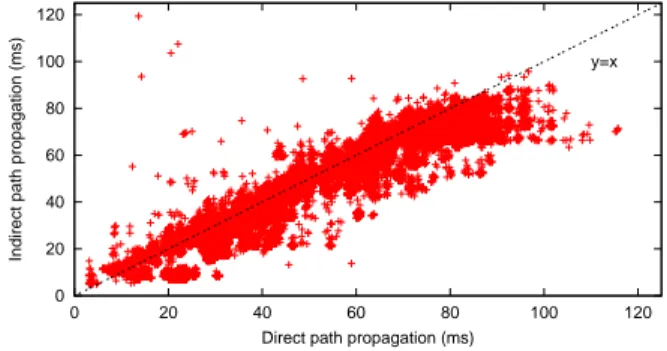
0 20 40 60 80 100 120 0 20 40 60 80 100 120
Indirect path propagation (ms)
Direct path propagation (ms)
y=x
Figure 12: “Circuitousness” of routes: Figure plotting the propagation delay of the best indirect path (y-axis) against the best multihoming path (x-axis).
Finally, if we consider the propagation delay of the best indirect overlay path versus the best multihoming path, we can get some idea of the relative ability to avoid overly “circuitous” paths, arising from policy routing, for example. Figure 12 shows a scatter plot of the propagation delay of the best direct path from a city (x-axis) and the best propagation delay via an indirect path (y-axis). Again, points below they = xline are cases in which overlay routing finds shorter paths than conventional BGP routing, and vice versa. Consistent with the earlier results, we see that the majority of points lie below they = xline where overlays find lower propagation delay paths. Moreover, for cases in which the direct path is shorter (above they=xline), the difference is generally small, roughly 10-15ms along most of the range.
Summary. A vast majority of RTT performance improvements
from overlay routing arise from its ability to find shorter end-to-end paths compared to the best direct BGP paths. However, the most significant improvements (>50ms) stem from the ability of overlay routing to avoid congested ISP links4.
5.8.2
Inter-domain and Peering Policy Compliance
To further understand the performance gap between some over-lay routes and direct BGP routes, we categorize the overover-lay routes by their compliance with common inter-domain and peering poli-cies. Inter-domain and peering policies typically represent business arrangements between ISPs [11, 20]. Because end-to-end overlay paths need not adhere to such policies, we try to quantify the per-formance gain that can be attributed to ignoring them.
Two key inter-domain policies [12] are valley-free routing — ISPs generally do not provide transit between their providers or peers because it represents a cost to them; and prefer customer — when possible, it is economically preferable for an ISP to route traffic via customers rather than providers or peers, and peers rather than providers. In addition, Spring et al. [28] observed that ISPs
of-4
The improvements from overlay routing could also be from over-lays choosing higher bandwidth paths. This aspect is difficult to quantify and we leave it as future work.
ten obey certain peering policies. Two common policies are early exit — in which ISPs “offload” traffic to peers quickly by using the peering point closest to the source; and late exit — some ISPs co-operatively carry traffic further than they have to by using peering points closer to the destination. BGP path selection is also impacted by the fact that the routes must have the shortest AS hop count.
We focus on indirect overlay paths (i.e.,> 1virtual hop) that provide better end-to-end round-trip performance than the corre-sponding direct BGP paths. To characterize these routes, we iden-tified AS level paths using traceroutes performed during the same period as the turnaround time measurements. Each turnaround time measurement was matched with a traceroute that occurred within 20 minutes of it (2.7% did not have corresponding traceroutes and were ignored in this analysis). We map IP addresses in the tracer-oute data to AS numbers using a commercial tool which uses BGP tables from multiple vantage points to extract the “origin AS” for each IP prefix [2]. One issue with deriving the AS path from tracer-outes is that these router-level AS paths may be different than the actual BGP AS path [18, 5, 14], often due to the appearance of an extra AS number corresponding to an Internet exchange point or a sibling AS5. In our analysis, we omit exchange point ASes, and also combine the sibling ASes, for those that we are able to identify. To ascertain the policy compliance of the indirect overlay paths, we used AS relationships generated by the authors of [31] during the same period as our measurements.
In our AS-level overlay path construction, we ignore the ASes of intermediate overlay nodes if they were used merely as non-transit hops to connect overlay path segments. For example, consider the overlay path between a source in ASS1and a destination inD2, composed of the two AS-level segmentsS1 A1 B1 C1andC1 B2 D2, where the intermediate node is located inC1. If the time spent inC1is short (< 3ms), andB1andB2are the same ISP, we consider the AS path asS1 A1 B1 D2, otherwise we con-sider it asS1 A1 B1 C1 B2 D2. Since we do this only for in-termediate ASes that are not a significant factor in the end-to-end round-trip difference, we avoid penalizing overlay paths for pol-icy violations that are just artifacts of where the intermediate hop belongs in the AS hierarchy.
Table 3 classifies the indirect overlay paths by policy confor-mance. As expected, the majority of indirect paths (70%) violated either the valley-free routing or prefer customer policies. How-ever, a large fraction of overlay paths (22%) appeared to be policy compliant. We sub-categorize the latter fraction of paths further by examining which AS-level overlay paths were identical to the AS-level direct BGP path and which ones were different.
For each overlay path that was identical, we characterized it as exiting an AS earlier than the direct path if it remained in the AS for at least 20ms less than it did in the direct path. We characterized it as exiting later if it remained in an AS for at least 20ms longer. We consider the rest of the indirect paths to be “similar” to the direct BGP paths. We see that almost all identical AS-level overlay paths either exited later or were similar to the direct BGP path. This suggests that cooperation among ISPs, e.g., in terms of late exit policies, can improve performance on BGP routes and further close the gap between multihoming and overlays. We also note that for the AS-level overlay paths that differed, the majority were the same length as the corresponding direct path chosen by BGP.
5
Two ASes identified as peers may actually be siblings [31, 11], in which case they would provide transit for each other’s traffic because they are administered by the same entity. We classified peers as siblings if they appeared to provide transit in the direct BGP paths in our traceroutes, and also manually adjusted pairings that were not related.
Improved Overlay Paths >20ms Imprv Paths
% RTT Imprv (ms) % RTT Imprv (ms)
Avg 90th Avg 90th
Violates Inter-Domain Policy 69.6 8.6 17 70.4 37.6 46 Valley-Free Routing 64.1 8.5 17 61.6 36.7 45 Prefer Customer 13.9 9.1 17 15.3 51.4 76
Valid Inter-Domain Path 22.0 7.3 15 19.4 38.8 49
Same AS-Level Path 13.3 6.9 13 10.2 42.6 54 Earlier AS Exit 1.6 5.3 8 0.7 54.1 119 Similar AS Exits 6.1 6.4 12 5.8 39.3 53 Later AS Exit 5.6 7.8 14 3.8 45.6 57 Diff AS-Level Path 8.8 8.0 17 9.2 34.7 44 Longer than BGP Path 1.9 9.9 20 3.5 32.3 39 Same Len as BGP Path 6.4 7.6 16 5.5 36.2 45 Shorter than BGP Path 0.5 5.4 11 0.1 35.8 43
Unknown 8.4 10.2
Table 3: Overlay routing policy compliance: Breakdown of the mean and 90th percentile round trip time improvement of in-direct overlay routes by: (1) routes did not conform to com-mon domain policies, and (2) routes that were valid inter-domain paths but either exited ASes at different points than the direct BGP route or were different than the BGP route.
Summary. In achieving better RTT performance than direct BGP
paths, most indirect overlay paths violate common inter-domain routing policies. We observed that a fraction of the policy-compliant overlay paths could be realized by BGP if ISPs employed coopera-tive peering policies such as late exit.
6.
RESILIENCE TO PATH FAILURES
BGP’s policy-based routing architecture masks a great deal of topology and path availability information from end-networks in order to respect commercial relationships and limit the impact of local changes on neighboring downstream ASes [10, 22]. This de-sign, while having advantages, can adversely affect the ability of end-networks to react quickly to service interruptions since noti-fications via BGP’s standard mechanisms can be delayed by tens of minutes [16]. Networks employing multihoming route control can mitigate this problem by monitoring paths across ISP links, and switching to an alternate ISP when failures occur. Overlay net-works provide the ability to quickly detect and route around failures by frequently probing the paths between all overlay nodes.
In this section, we perform two separate, preliminary analyses to assess the ability of both mechanisms to withstand end-to-end path failures and improve availability of Internet paths. The first ap-proach evaluates the availability provided by route control based on active probe measurements on our testbed. In the second we com-pute the end-to-end path availability from both route control and overlays using estimated availabilities of routers along the paths.
6.1
Active Measurements of Path Availability
In our first approach, we perform two-way ICMP pings between the 68 nodes in our testbed. The ping samples were collected be-tween all node-pairs over a five day period from January 23rd, 2004 to January 28th, 2004. The probes are sent once every minute with a one second timeout. If no response is received within a second, the ping is deemed lost. A path is considered to have failed if≥3
consecutive pings (each one minute apart) from the source to the destination are lost. From these measurements we derive “failure epochs” on each path. The epoch begins when the third failed probe times out, and ends on the first successful reply from a subsequent probe. These epochs are the periods of time when the route be-tween the source and destination may have failed.
This method of deriving failure epochs has a few limitations.
Firstly, since we wait for three consecutive losses, we cannot detect failures that last less than 3 minutes. As a result, our analysis does not characterize the relative ability of overlays and route control to avoid such short failures. Secondly, ping packets may also be dropped due to congestion rather than path failure. Unfortunately, from our measurements we cannot easily determine if the losses are due to failures or due to congestion. Finally, the destination may not reply with ICMP echo reply messages within one second, caus-ing us to record a loss. To mitigate this factor, we eliminate paths for which the fraction of lost probes is>10%from our analysis. Due to the above reasons, the path failures we identify should be considered an over-estimate of the number of failures lasting three minutes or longer.
From the failure epochs on each end-to-end path, we compute the corresponding availability, defined as follows:
Availability = 100× 1− P iTF(i) T
where,TF(i)is the length of failure epochialong the path, and Tis the length of the measurement interval (5 days). The total sum of the failure epochs can be considered the observed “downtime” of the path. 0 0.05 0.1 0.15 0.2 0.25 0.3 99.5 99.55 99.6 99.65 99.7 99.75 99.8 99.85 99.9 99.95 100
Fraction of paths with Availability < x
Availability (percentage) No multihoming
2-multihoming 3-multihoming
Figure 13: End-to-end failures: Distribution of the availability on the end-to-end paths, with and without multihoming. The ISPs in the 2- and 3-multihoming cases are the best 2 and 3
ISPs in each city based on RTT performance, respectively. k
-Overlay routing, for anyk, achieves 100% availability and is
not shown on the graph.
In Figure 13, we show a CDF of the availability on the paths we measured, with and without multihoming. When no multihoming is employed, we see that all paths have at least91%availability (not shown in the figure). Fewer than 5%of all paths have less than99.5% availability. Route control with multihoming signifi-cantly improves the availability on the end-to-end paths, as shown by the 2- and 3-multihoming availability distributions. Here, for both 2- and 3-multihoming, we consider the combinations of ISPs providing the best round-trip time performance in a city. Even when route control uses only 2 ISPs, less than 1%of the paths originating from the cities we studied have an availability under
99.9%. The minimum availability across all the paths is99.85%, which is much higher than without multihoming. Also, more than
94%of the paths from the various cities to the respective destina-tions do not experience any observable failures during the 5 day period (i.e.,availability of100%). With three providers, the avail-ability is improved, though slightly. Overlay routing may be able to circumvent even the few failures that route control could not avoid. However, as we show above, this would result in only a
marginal improvement over route control which already offers very good availability.
6.2
Path Availability Analysis
Since the vast majority of paths did not fail even once during our relatively short measurement period, our second approach uses statistics derived from previous long-term measurements to ascer-tain availability. Feamster et al. collected failure data using active probes between nodes in the RON testbed approximately every 30 seconds for several months [9]. When three consecutive probes on a path were lost, a traceroute was triggered to identify where the failure appeared (i.e., the last router reachable by the traceroute) and how long they lasted. The routers in the traceroute data were also labeled with their corresponding AS number and also classi-fied as border or internal routers. We use a subset of these measure-ments on paths between non-DSL nodes within the U.S. collected between June 26, 2002 and March 12, 2003 to infer failure rates in our testbed. Though this approach has some drawbacks (which we discuss later), it allows us to obtain a view of longer-term availabil-ity benefits of route control and overlay routing that is not otherwise possible from direct measurements on our testbed.
We first estimate the availabilities of different router classes (i.e., the fraction of time they are able to correctly forward packets). We classify routers in the RON traceroutes by their AS tier (using the method in [31]) and their role (border or internal router). Note that the inference of failure location is based on router location, but the actual failure could be at the link or router attached to the last responding router.
The availability estimate is computed as follows: IfP
TC F is the total time failures attributed to routers of classCwere observed, andNC
d is the total number of routers of classCwe observed on each path on dayd,6then we estimate the availability of a router (or attached link) of classCas:
AvailabilityC = 100× 1− PTC F P dN C d ×one day
In other words, the fraction of time unavailable is the aggregate failure time attributed to a router of classC divided by the total time we expect to observe a router of classC in any path. Our estimates for various router classes are shown in Table 4.
AS Tier Location Availability (%)
1 internal 99.940 1 border 99.985 2 internal 99.995 2 border 99.977 3 internal 99.999 3 border 99.991 4 internal 99.946 4 border 99.994 5 internal 99.902 5 border 99.918
Table 4: Availability across router classes: Estimated availabil-ity for routers or links classified by AS tier and location. We consider a border router as one with at least one link to an-other AS.
To apply the availability statistics derived from the RON data set, we identified and classified the routers on paths between nodes
6
The dataset only included a single successful traceroute per day. Therefore, we assumed that all active probes took the same route each day.
in our testbed. We performed traceroute measurements approxi-mately every 20 minutes between nodes in our CDN testbed from December 4, 2003 to Dec 11, 2003. For our analysis we used the most often observed path between each pair of nodes; in almost all cases, this path was used more than 95% of the time. Using the router availabilities estimated from the RON data set, we estimate the availability of routes in our testbed when we use route control or overlay routing. When estimating the simultaneous failure prob-ability of multiple paths, it is important to identify which routers are shared among the paths so that failures on those paths are accu-rately correlated. Because determining router aliases was difficult on some paths in our testbed,7we conservatively assumed that the routers at the end of paths toward the same destination were identi-cal if they belonged to the same sequence of ASes. For example, if we had two router-level paths destined for a common node that map to the ASesA A B B C CandD D D B C C, respectively, we assume the last 3 routers are the same (sinceB C Cis common). Even if in reality these routers are different, failures at these routers are still likely to be correlated. The same heuristic was used to identify identical routers on paths originating from the same source node. We assume other failures are independent.
A few aspects of this approach may introduce biases in our anal-ysis. First, the routes on RON paths may not be representative of the routes in our testbed, though we tried to ensure similarity by us-ing only usus-ing paths between relatively well-connected RON nodes in the U.S. In addition, we observed that the availabilities across router classes in the RON dataset did not vary substantially across different months, so we do not believe the difference in timeframes impacted our results. Second, there may be routers or links in the RON data set that fail frequently and bias the availability of a par-ticular router type. However, since traceroutes are initiated only when a failure is detected, there is no way for us to accurately es-timate the overall failure rates of all individual routers. Third, it is questionable whether we should assign failures to the last reach-able router in a traceroute; it is possible that the next (unknown) or an even further router in the path is actually the one that failed. Nevertheless, our availabilities still estimate how often failures are observed at or just after a router of a given type.
Figure 14 compares the average availability using overlays and route control on paths originating from 6 cities to all destinations in our testbed. For overlay routing, we only calculate the availability of the paths for the first and last overlay hop (since these will be the same no matter which intermediate hops are used), and assume that there is always an available path between other intermediate hops. An ideal overlay has a practically unlimited number of path choices, and can avoid a large number of failures in the middle of the network.
As expected from our active measurements, the average avail-ability along the paths in our testbed are relatively high, even for direct paths. 3-multihoming improves the average availability by 0.15-0.24% in all the cities (corresponding to about 13-21 more hours of availability each year). Here, the availability is primarily upper bounded by the availability of the routers or links immedi-ately before the destination that are shared by all three paths as they converge.
In most cases, 1-overlays have slightly higher availability (at most about 0.07%). Since a 1-overlay has arbitrary flexibility in choosing intermediate hops, only about 2.7 routers are common (on average) between all possible overlay paths, compared to about 4.2 in the 3-multihoming case. However, note that a 1-overlay path using a single provider is more vulnerable to access link failures
7
We found that several ISPs block responses to UDP probe packets used by IP alias resolution tools such as Ally [29]