Enhanced Framework of Quantum Approximate Optimization
Algorithm and Its Parameter Setting Strategy
Mingyou Wu
1, Zhihao Liu
1,2, and Hanwu Chen
1,21School of Computer Science and Engineering, Southeast University, Nanjing 211189, China
2Key Laboratory of Computer Network and Information Integration (Southeast University), Ministry of Education, Nanjing, 211189, China
December 18, 2020
Abstract
An enhanced framework of quantum approximate optimization algorithm (QAOA) is introduced and the parameter setting strategies are analyzed. The enhanced QAOA is as effective as the QAOA but exhibits greater computing power and flexibility, and with proper parameters, it can arrive at the optimal solution faster. Moreover, based on the analysis of this framework, strategies are provided to select the parameter at a cost of O(1). Simulations are conducted on randomly generated 3-satisfiability (3-SAT) of scale of 20 qubits and the optimal solution can be found with a high probability in iterations much less thanO(√N)
1
Introduction
In 2014, Farhiet al. [1] proposed a quantum classical hybrid variational method, the quantum approximate optimization algorithm (QAOA) for combinatorial optimization problems (COP). The QAOA defines the problem HamiltonianHC and use the transverse field as the mix HamiltonianHB. These two Hamiltonians
are alternately applied to the quantum state and the evolution timeγ andβ are introduced as parameters. With proper parameters, the expectation of the quantum state gradually grows and after enough iterations, the optimal solution will be obtained.
Recently, Farhiet al. [2] pointed out that the QAOA need to see the whole graph and used the QAOA+ as an example. The QAOA+ adopts the information of graph structure into the problem Hamiltonian instead of preparing a specific initial state. Based on the comparison between QAOA and QAOA+ on maximum independent set (MIS), an enhanced framework of QAOA is proposed, which is effective and more flexible. Besides, the complexity of the enhanced QAOA is analyzed and a parameter initial strategy of costs of
O(1) is provided. This strategy naturally applies to 3-satisfiability (3SAT) and in a single simulation the satisfiability can be determined with a probability around 50% for O(nlogm) iterations, where m is the number of constraints valued inO(n3). For general NP-complete problem, a reduction to 3-SAT is always available, and strategies are advised to adjust the parameters.
The reminder of this paper is o rganized as follows. Section 2 briefly reviews the QAOA and QAOA+ for MIS. In Section 3, a basis is introduced and developed on this, the enhanced QAOA is proposed and ana-lyzed. Section 4 presents the practical meaning and the setting strategies of parameters, and corresponding simulations are conducted. Finally, Section 5 concludes this paper.
2
Review of the QAOA
For a combinatorial optimization problem of scalenwithmclauses, the objective function can be expressed as follows: C(z) = m X α=1 Cα(z), (1)
where stringz∈ {0,1}n andCαstands for a certain clauseα,
Cα=
1 ifzsatisfies the clauseα,
0 if zdoes not satisfy. (2) COP asks for a stringz that maximizes the objective functionC(z). And the approximate optimization demands a stringz for whichC(z) is close to the optimal ofC.
In the QAOA, the initial state is usually the equal superposition state
|si= √1
2n
X
j
|ji. (3)
And the evolution operators of QAOA is a series of operators interleaved withUC(γ) =e−iγHC andUB(γ) =
e−iβHB. γ andβ are parameters between 0 and 2π and varies during the procedure of QAOA. H
C is the
problem Hamiltonian which is determined by the problem as
HC=diag{C(zi)}, (4)
andHB is the mix Hamiltonian, which usually is the transverse field written as
HB=
X
j
σxj. (5)
Forpiterations the system state is
|zpi=UB(βp)UC(γp). . . UB(β1)UC(γ1)|si, (6)
and herepis call the depth of QAOA.|zpican also be denoted as |γ, βi, and the expectation of state |zpi
onHC is
Fp(γ, β) =hγ, β|HC|γ, βi. (7)
Fp(γ, β) can be used to select the parameters such thatFp−1(γ, β)< Fp(γ, β).
The maximum independent set (MIS) problem asks for the independent set of the largest possible size for the given graph. Farhi [1] first applies the QAOA to the MIS, and use
C(z) =X
jzj (8)
as the objective function. This definition only considers the number of vertices in each solution, so a special-ized initial state is required, and the quantum adiabatic algorithm is applied to prepare the superposition of all feasible solutions. Recently Farhi [2] suggested that the QAOA should consider the whole graph, and put forward the QAOA+ with a new objective function
C+(z) = X jzj− X u,v Au,vzuzv, (9)
where Au,v is the element of the adjacent matrix of given graph. This objective function considers the
basic structure of the graph and has a more powerful computing power, which can handle the MIS problem without the help of an appended initial state preparation.
3
The enhanced framework of QAOA
Considering the problem Hamiltonians of QAOA and QAOA+ for MIS, the detailed expression is
HC=P k Pk, HC+=P k Pk−P u,v Au,vPu,v, (10)
where Pk denotes operatorP =diag{0,1} on thek-th qubit,Pu,v denotesP on the u-th andv-th qubits,
andAu,v is the element of the adjacent matrix of graph. Both the problem Hamiltonians can be expressed
as a linear combination of projection operators. Expand these projection operators to
pj =⊗ni=1(Pi) ji = (P 1) ji⊗(P 2) j2⊗. . .⊗(P n) jn. (11)
LetZi denoteZ on thei-th qubit. The Walsh operator [3] onnqubits is
wj=⊗ni=1(Zi) ji = (Z 1) ji⊗(Z 2) j2⊗. . .⊗(Z n) jn. (12)
Actually,Z =I−2Pi, andwj can be represented by pj. wj is an orthonormal basis of dialog matrixes of
dimension 2n ande−iθjwj can be implemented by (n) basic gates [3]. Obviously,p
j also consists a basis and
the implementation cost ofe−iγjpj isO(n) [4].
Therefore, the unitary operator of any problem Hamiltonian can be rewritten as
UC(γ) =e−i
PN−1
j=0 γpj. (13)
Replacingγ in Eq. (13) withγj, a new unitary operator can be written as
UCe(γ) =e−i
PN−1
j=0 γjpj. (14)
This is the original idea and basic form of the enhanced QAOA. The evolution operatore−iγHC is replaced
by a sequence of control evolution gates that
CRj(γ) =e−iγjpj, (15)
where if thex-th qubit is a control qubit, thenjx= 1. In fact, for the Hamiltonian of majority of COP only
a few bases in{pj} are used. Therefore, the layer of QAOA is defined as the maximum ofd(j) of all control
evolution gates, where
d(j) =
n
X
x=1
jx (16)
is the number of control bits.
Denote COP with constraints that engage no more than k variables as COPk. Without an extern
computing power or extra information, a k-layer QAOA can solve COPk but cannot deal with COPk+1.
MIS after specific initial state preparation is inCOP1. In fact, the evolution operators of 1-layer QAOA are
local on a single qubit and the entanglement is invariable. It means the 1-layer QAOA does not provide any computation power, but only present the computation basis closest to the optimal solution. NP-complete problem and COP2 can reduce to each other in polynomial time. In fact, max-cut is in COP2 and every
problem inCOP2 can be reduced as a max-cut problem on a weighted graph with loop. COPk is the
NP-optimization problem for a constant k such as MIS, 3SAT and E3Lin2 [5]. COPn is the hardest COP of
scale n. In classical computer, it cost exponentially to evaluate the quality of a solution, and in quantum computer, the cost of the implementation of theUC is also exponential.
It is clear that the enhanced QAOA has a similar framework to QAOA with the same implementation cost, and the parameterγγγ = (γj) enables the Hamiltonian to vary in a larger space which would result in
an increase of the computation capability. For example, consider a simple comparison between the standard QAOA and the enhanced QAOA of 1-layer for the MIS, and theHC can be respectively written as
HCs=P j Pj, HCg=P j γjPj. (17)
Because of the lack of control evolution gates thatd(l) = 2, the 1-layer standard QAOA of nqubits cannot represent majority of the constraints and is unable to deal with MIS of scalen. As for the enhanced QAOA, with specific selected parameters γγγ, the enhanced QAOA can solve MIS by increasing the parameters of the bases that contain vertices in maximum independent set and decreasing the others. For this case, the computation capability of the 1-layer enhanced QAOA mainly comes from the parameters setting, i. e., the parameters optimizer, and the correctness mainly depends on the optimizer. The interface of the enhanced QAOA available for classical computing power increases and so is the computation capability. But when applying the enhanced QAOA to certain problem, the quantum computation capability ought to be the main component to execute the calculation task, and the classical computer provides assistance, so the layer should be at least as the same as the standard QAOA.
For a fixed layer, the enhanced QAOA can arrive at the target state faster than the standard QAOA. Obviously, the enhanced QAOA cannot be slower than the standard QAOA. For convenience, the parameters
γγγare decomposed into two parts asγγγ=γsγγγrrr, whereγsis the global phase, andγγγrrris the relative phase. The
parametersγγγrrrof the standard QAOA are determined by the constraints and are static during the evolution
of algorithm. Use contradiction and suppose the enhanced QAOA is as fast as the standard QAOA. When optimizing the expectationF(γs, γγγrrr),Fm(γs) should be equal toFm(γs, γγγrrr), that is
∂F(γs, γγγrrr)
∂γγγrrr
=∂F(γs)
∂γγγrrr
= 0, (18)
that is,γγγrrr is independent toF(γs, γγγrrr). This is obviously wrong, such as the 1-layer standard and enhanced
QAOA on MIS, and the latter can arrive a larger expectation.
4
Parameter setting and simulation result
Consider the normalization ofγγγrrr. Firstly, the Grover Hamiltoniandiag{1,0, . . . ,0}[6] applied as a search of
QAOA [7] should be normalized and so is the multi-solutions case. And withγs=π,U(HC, γγγ) can best
dis-tinguish the optimal and non-optimal solutions. For general case, the best normalization is linearly mapping the goal values of solutions from [Cmin, Cmax] to [0,1]. However, Cmax cannot be directly normalized to 1
because the value ofCmax is the algorithm target. Instead, Clim =Pjγr,j is adopted andClim ≥Cmax.
Therefore,P
jγr,j should be normalized to 1 and when negative constraints are occupied,Pj|γr,j|= 1.
This normalization strategy naturally applies to satisfiability problem. Using 3-SAT as example, problem is satisfiable ifClim=Cmax, that is, the maximum of the eigenvalue of normalized Hamiltonian is 1. Noting
the periodicity of e−iθ, with parameter γ
s = (2t+ 1)π and any t ∈z, the effective phase shift of optimal
solution is always π, but that of the non-optimal solution varies with the change oft. By modifyingt, the angle between the optimal and non-optimal solution would increase. As for unsatisfiable case, the larger the difference between Clim and Cmax, the smaller the probability to find the solution of Cmax. The CTQW
part actually has the form of
e−iβHB =He−iβHZH, (19) where HZ= n−1 X m=0 Zm (20)
andZmisZ on them-th qubit. Therefore, 1/nis a good parameter forβ because the eigenvalue ofHZ can
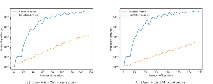
0 20 40 60 80 100 120 140 160 Number of iterations 106 105 104 103 102 101 Probability of target Satisfied cases Unsatified cases
(a) Case with 2M constraints
0 25 50 75 100 125 150 175 Number of iterations 106 105 104 103 102 101 Probability of target Satisfied cases Unsatified cases
(b) Case with 4M constraints
Figure 1: The average probability of the target computational basis during iterations.
Table 1: The average of the maximum probability of target during iterations. constraints 2M&satisfied 2M&unsatisfied 4M&satisfied 4M&unsatisfied max probability 0.4392 0.0018 0.4747 0.0003
set to benlogm/√2 and the maximum oft is logm, namely, forp-depth QAOA,
γ= $ 2√2p n % + 1 ! π, (21)
where 1≤p≤ nlogm/√2 . The simulation results of scale of 20 qubits on randomly generated instance of 3-SAT are shown in Figure 1 and Table 1. For satisfied case, firstly the solution as randomly selected and then the constraints satisfied by the solution are randomly generated. And for unsatisfied case, the constraints are randomly generated and the satisfied instances are excluded. The number of constraints values 2M and 4M and both satisfied and unsatisfied cases are considered, where M =C3
20. The number
of repeated experiments is 50 times for each case. In fact, a fewer number iterations is also feasible as
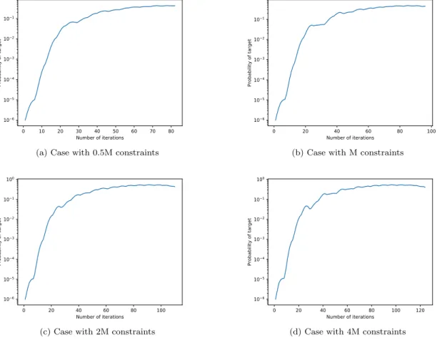
nlog (2m/n)/√2 and the maximum of t is log (2mn). The simulation results are shown in Figure 2 and Table 2. The number of constraints values 0.5M, M, 2M and 4M and only satisfied case are presented.
However, for general COP, a satisfiable solution is very rare, this is,Cmaxis generally much smaller than
Clim. Noting the difference ∆C=|Clim−Cmax|, with the growth of the scale of problem, the depth required
to arrive the optimal solution increases, and the influence of ∆C on optimization might become greater and
unpredictable. Therefore, specific strategies are required to adjust the Hamiltonian. In fact, the range of the solution of a specific COP can be obtained by probability theory and combinatorial Mathematics, and can be adopted as prior knowledge. By multiplying a specific factor which can be gradually adjusted, the maximum of the eigenvalue of problem Hamiltonian can be approximately normalized to 1. Besides, the measurement resultej(z) =hz|pj|zi of repeat experiments presents the importance ofpj and can be used to adjust the
parametersγr,j. And the normalized
eα
jγr,j can be adopted as the parameters of next experiment, where
αis the adjusting factor andα≥0.
Table 2: The average of the maximum probability for a decreased iterations. constraints 0.5M M 2M 4M
0 10 20 30 40 50 60 70 80 Number of iterations 106 105 104 103 102 101 Probability of target
(a) Case with 0.5M constraints
0 20 40 60 80 100 Number of iterations 106 105 104 103 102 101 Probability of target
(b) Case with M constraints
0 20 40 60 80 100 Number of iterations 106 105 104 103 102 101 100 Probability of target
(c) Case with 2M constraints
0 20 40 60 80 100 120 Number of iterations 106 105 104 103 102 101 100 Probability of target
(d) Case with 4M constraints
Figure 2: The average probability of the target computational basis for a decreased iterations.
5
Discussion and conclusion
The enhanced QAOA introduced in this paper inherits the properties of the QAOA without any extra cost, and moreover, exhibits many superiorities. The parametersγ andβ of the standard QAOA is actually the evolution time and the problem Hamiltonian is static during the iterations. However, with the additional parametersγγγrrr, the enhanced QAOA can adjust the problem Hamiltonian during algorithm process, which
can reduce the complexity and provides interface for classical computing power. Furthermore, the extra computation capability is adjustable and offers more options for researchers. This paper defines the layer of the QAOA that determines the upper bound of the implementation complexity, and presents a series of problemsCOPk that reflect the upper bound of the computability of the QAOA of certain layer. Meanwhile,
the QAOA of different layers also provides reference models for the corresponding problems. QAOA provides a scheme combining quantum and classical computing power, while the enhanced QAOA presents a new view for the architecture of the QAOA, and would be useful to reconsider and organize the previous work.
This enhanced framework of the QAOA more clearly shows the piratical meaning of the parameters and based on this, parameter setting strategies of the enhanced QAOA are proposed. The simulation shows its efficiency on 3-SAT, but limited by the simulation complexity of quantum system, only cases with 20 qubits are analysis. Further experimental and theoretical analysis are urgently required. Besides, the enhanced QAOA reveals other issues like the analysis of the alteration of Hamiltonian under certain parameter setting strategy. Nevertheless, the enhanced QAOA does not show advantage on matters like the depth analysis of QAOA, the standard QAOA is still needed in some theoretical derivation.
References
[1] Edward Farhi, Jeffrey Goldstone and Sam Gutmann, A Quantum Approximate Optimization Algorithm,
arXiv, quant-ph, 1411.4028 (2014).
[2] Edward Farhi, David Gamarnik and Sam Gutmann, The Quantum Approximate Optimization Algo-rithm Needs to See the Whole Graph: A Typical Case,arXiv, quant-ph, 2004.09002, (2020).
[3] Jonathan Welch, Daniel Greenbaum, Sarah Mostame and Alan Aspuru-Guzik, Efficient quantum circuits for diagonal unitaries without ancillas,New J. Phys.16033040 (2014).
[4] Qing Lin, Multiple multicontrol unitary operations: Implementation and applications, Science China
Physics, Mechanics & Astronomy,61, 040314 (2018)
[5] Edward Farhi and Jeffrey Goldstone and Sam Gutmann, A Quantum Approximate Optimization Algo-rithm Applied to a Bounded Occurrence Constraint Problem,arXiv, quant-ph, 1412.6062 (2015). [6] Lov K. Grover, Quantum Mechanics Helps in Searching for a Needle in a Haystack, Physical Review
Letters, 79p. 325 (1997).
[7] Zhang Jiang, Eleanor G. Rieffel and Zhihui Wang, Near-optimal quantum circuit for Grover’s unstruc-tured search using a transverse field,Physical Review A,95 p. 062317 (2017).