Module 5: Normalization of database tables
•
Normalization
is a process for evaluating and correcting
table structures to minimize data redundancies, thereby
reducing the likelihood of data anomalies.
•
The normalization process involves assigning attributes to
entities.
•
Normalization works through a series of stages called normal
forms:
▫ First normal form (1NF) ▫ Second normal form (2NF) ▫ Third normal form (3NF) ▫ Fourth normal form (4NF)
•
Although normalization is a very important database design
ingredient, you should not assume that the highest level of
normalization is always the most desirable.
The Need for Normalization
•
Normalization is typically used in conjunction with
the entity relationship modeling.
•
There are two common situations in which database
designers use normalization:
▫ designing a new database structure, or
▫ modifying an existing one
•
To get a better idea of the normalization process,
consider the simplified database activities of a
construction
company
that
manages
several
building projects.
Case of a Construction Company
▫
Building project
-- Project number, Name, Employees
assigned to the project.
▫
Employee
-- Employee number, Name, Job classification
▫
The company charges its clients by billing the hours spent
on each project. The hourly billing rate is dependent on the
employee’s position.
▫
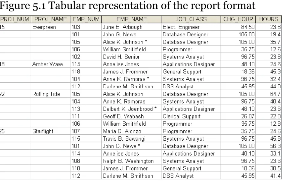
Periodically, a report is generated as shown in Table 5.1.
▫
The table whose contents correspond to the reporting
requirements is shown in Figure 5.1.
Scenario
•
A few employees work for one project
Employee Num : 101,
102, 103, 105 Project Num : 15
Project Name :
SAMPLE FORM
Project Num : 15
Project Name : Evergreen
Emp Num Emp Name Job Class Chr Hours Hrs Billed Total
101 102 103 105
Figure 5.1 Tabular representation of the report format
NOTE: The total charge in Table 5.1 is a derived attribute and, at this point, is not stored in the table.
Problems in Fig 5.1
•
Unfortunately, the structure of the dataset in
Figure 5.1 does not conform to the requirements
nor does it handle data very well. Consider the
following deficiencies:
1. The project number is intended to be a primary key, but it
contains nulls.
2. The table entries invite data inconsistencies.
For example, JOB_CLASS Elect. Engr. might be Elect.
Engineer, El. Eng or EE).
3. The table displays data redundancies which yield the
following anomalies:
Update anomalies. (ex. Modifying JOB_CLASS for EMP 105 requires many alterations, for each EMP 105.)
Addition anomalies. (Just to complete a row definition, a new employee must be assigned to a project. If the employee is not yet assigned, a phantom project must be created to complete the employee data entry.)
Deletion anomalies. Suppose that only one employee is associated with a given project. If that employee leaves the company and the employee data are deleted, the project information will also be deleted. To prevent the loss of the project information, a fictitious employee must be created just to save the project information.
The Normalization Process
• The objective of normalization is to ensure that each table conforms to the concept of well-formed relations—that is, tables that have the following characteristics:
• Each table represents a single subject. For example, a course table will contain only data that directly pertain to courses. Similarly, a student table will contain only student data.
• No data item will be unnecessarily stored in more than one table (in short, tables have minimum controlled redundancy). The reason for this requirement is to ensure that the data are updated in only one place.
• All nonprime attributes in a table are dependent on the primary key—the entire primary key and nothing but the primary key. The reason for this requirement is to ensure that the data are uniquely identifiable by a primary key value.
• Each table is void of insertion, update, or deletion anomalies. This is to ensure the integrity and consistency of the data.
•
To accomplish the objective, the normalization
process takes you through the steps that lead to
successively higher normal forms. The most
common
normal
forms
and
their
basic
characteristic are listed in Table 5.2.
NORMAL FORM CHARACTERISTIC
First normal form (1NF) Table format, no repeating groups, and PK identified
Second normal form (2NF) 1NF and no partial dependencies Third normal form (3NF) 2NF and no transitive dependencies Boyce-Codd normal form (BCNF) Every determinant is a candidate key
(special case of 3NF)
Fourth normal form (4NF) 3NF and no independent multivalued dependencies
•
The concept of keys is central to the discussion
of normalization.
•
Recall from Chapter 3 that a candidate key is a
minimal (irreducible) superkey. The primary key
is the candidate key that is selected to be the
primary means used to identify the rows in the
table.
•
From the data modeler’s point of view, the
objective of normalization is to ensure that all
tables are at least in third normal form (3NF).
FUNCTIONAL DEPENDENCE
•
Recall from Module 3 the concepts of determination and
functional dependence.
•
•
CONCEPT DEFINITION
Functional Dependence The attribute B is fully functionally dependent on the attribute A if each value of A determines one and only one value of B.
Example: PROJ_NUM →PROJ_NAME
(read as “PROJ_NUM functionally determines PROJ_NAME”) In this case, the attribute PROJ_NUM is known as the
“determinant” attribute, and the attribute PROJ_NAME is known as the “dependent” attribute.
Functional dependence (generalized definition)
Attribute A determines attribute B (that is, B is functionally dependent on A) if all of the rows in the table that agree in value for attribute A also agree in value for attribute B.
Fully functional dependence (composite key)
If attribute B is functionally dependent on a composite key A but not on any subset of that composite key, the attribute B is fully functionally dependent on A.
•
It is crucial to understand these concepts
because they are used to derive the set of
functional dependencies for a given relation.
•
The normalization process works one relation at
a time, identifying the dependencies on that
relation and normalizing the relation.
•
Normalization
starts
by
identifying
the
dependencies
of
a
given
relation
and
progressively breaking up the relation (table)
into a set of new relations (tables) based on the
identified dependencies.
• Two types of functional dependencies that are of special interest in normalization are partial dependencies and transitive dependencies.
1. partial dependency exists when there is a functional dependence in which the determinant is only part of the primary key (remember we are assuming there is only one candidate key).
For example, if (A, B) → (C,D), B → C, and (A, B) is the primary key, then the functional dependence B → C is a partial dependency because only part of the primary key (B) is needed to determine the value of C. Partial dependencies tend to be rather straightforward and easy to identify.
2. transitive dependency exists when there are functional dependencies such that X → Y, Y → Z, and X is the primary key.
In that case, the dependency X → Z is a transitive dependency because X determines the value of Z via Y. Unlike partial dependencies, transitive dependencies are more difficult to identify among a set of data. Fortunately, there is an easier way to identify transitive dependencies. A transitive dependency will occur only when a functional dependence exists among nonprime attributes.
Conversion to First Normal Form(1NF)
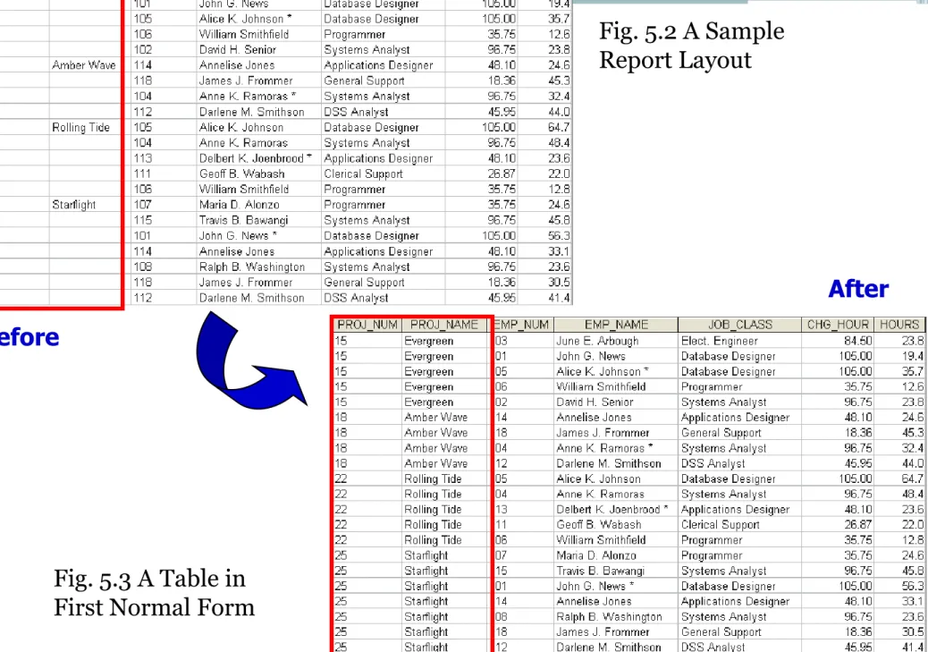
• In Figure 5.1, note that each single project number (PROJ_NUM) occurrence can reference a group of related data entries.
For example, the Evergreen project (PROJ_NUM = 15) shows five entries at this point—and those entries are related because they each share the PROJ_NUM = 15 characteristic. Each time a new record is entered for the Evergreen project, the number of entries in the group grows by one.
• A repeating group derives its name from the fact that a group of multiple entries of the same type can exist for any single key attribute occurrence.
• A relational table must not contain repeating groups. The existence of repeating groups provides evidence that the RPT_FORMAT table in Figure 5.1 fails to meet even the lowest normal form requirements, thus reflecting data redundancies.
•
Normalizing the table structure will reduce the data
redundancies.
•
If repeating groups do exist, they must be eliminated
by making sure that each row defines a single entity.
•
In addition, the dependencies must be identified to
diagnose the normal form.
•
Identification of the normal form will let you know
where you are in the normalization process.
•
The normalization process starts with a simple
Step 1: Eliminate the Repeating Groups
•
Start by presenting the data in a tabular format,
where each cell has a single value and there are
no repeating groups.
•
To eliminate the repeating groups, eliminate the
nulls by making sure that each repeating group
attribute contains an appropriate data value.
Before
After
Fig. 5.3 A Table in First Normal Form
Fig. 5.2 A Sample Report Layout
Step 2: Identify the Primary Key
•
The layout in Figure 5.3 represents more than a mere
cosmetic change.
•
Even a casual observer will note that PROJ_NUM is not an
adequate primary key because the project number does not
uniquely identify all of the remaining entity (row) attributes.
For example, the PROJ_NUM value 15 can identify any one of
five employees.
•
To maintain a proper primary key that will uniquely identify
any attribute value, the new key must be composed of a
combination of PROJ_NUM and EMP_NUM.
•
For example, using the data shown in Figure 5.3, if you know
that PROJ_NUM = 15 and EMP_NUM = 103, the entries for
the attributes PROJ_NAME, EMP_NAME, JOB_CLASS,
CHG_HOUR, and HOURS must be Evergreen, June E.
Arbough, Elect. Engineer, $84.50, and 23.8, respectively.
Step 3: Identify All Dependencies
•
The identification of the PK in Step 2 means that
you
have
already
identified
the
following
dependency:
PROJ_NUM, EMP_NUM
→
PROJ_NAME, EMP_NAME, JOB_CLASS,
CHG_HOUR, HOURS
•
That
is,
the
PROJ_NAME,
EMP_NAME,
JOB_CLASS, CHG_HOUR, and HOURS values are
all dependent on—that is, they are determined by—
the combination of PROJ_NUM and EMP_NUM.
Dependency Diagram
-
a diagram that depicts all dependencies found
within a given table structure.
•
Dependency diagrams are very helpful in getting a
bird’s-eye view of all of the relationships among a
table’s attributes, and their use makes it less likely
that you will overlook an important dependency.
Note the following dependency diagram features:
1.
The primary key attributes are bold, underlined,
and shaded in a different color.
2. The arrows above the attributes indicate all desirable dependencies, that is, dependencies that are based on the primary key.
In this case, note that the entity’s attributes are dependent on the combination of PROJ_NUM and EMP_NUM.
3. The arrows below the dependency diagram indicate less desirable dependencies. Two types of such dependencies exist:
a. Partial dependencies. You need to know only the PROJ_NUM to determine the PROJ_NAME; that is, the PROJ_NAME is dependent on only part of the primary key. And you need to know only the EMP_NUM to find the EMP_NAME, the JOB_CLASS, and the CHG_HOUR. A dependency based on only a part of a composite primary key is a partial dependency.
b. Transitive dependencies. Note that CHG_HOUR is dependent on JOB_CLASS. Because neither CHG_HOUR nor JOB_CLASS is a prime attribute—that is, neither attribute is at least part of a key—the condition is a transitive dependency. In other words, a transitive dependency is a dependency of one nonprime attribute on another nonprime attribute. The problem with transitive dependencies is that they still yield data anomalies.
1NF (PROJ_NUM, EMP_NUM, PROJ_NAME, EMP_NAME, PARTIAL DEPENDENCIES:
(PROJ_NUM PROJ_NAME)
(EMP_NUM EMP_NAME, JOB_CLASS, CHG_HOUR) TRANSITIVE DEPENDENCY
1NF Definition
•
The term
first normal form (1NF)
describes
the tabular format in which:
All of the key attributes are defined.
There are no repeating groups in the table. In
other words, each row/column intersection
contains one and only one value, not a set of
values.
All attributes are dependent on the primary
key.
• All relational tables satisfy the 1NF requirements.
• The problem with the 1NF table structure shown in Figure 5.4 is that it contains partial dependencies—that is, dependencies based on only a part of the primary key.
• While partial dependencies are sometimes used for performance reasons, they should be used with caution.
• Such caution is warranted because a table that contains partial dependencies is still subject to data redundancies, and therefore, to various anomalies. The data redundancies occur because every row entry requires duplication of data.
• For example, if Alice K. Johnson submits her work log, then the user would have to make multiple entries during the course of a day. For each entry, the EMP_NAME, JOB_CLASS, and CHG_HOUR must be entered each time, even though the attribute values are identical for each row entered. Such duplication of effort is very inefficient. What’s more, the duplication of effort helps create data anomalies; nothing prevents the user from typing slightly different versions of the employee name, the position, or the hourly pay.
• Such data anomalies violate the relational database’s integrity and consistency rules.
Conversion to Second Normal Form (2NF)
•
Converting to 2NF is done only when the 1NF
has a composite primary key.
•
If the 1NF has a single-attribute primary key,
then the table is automatically in 2NF.
•
The 1NF-to-2NF conversion is simple. Starting
with the 1NF format displayed in Figure 5.4, you
do the following:
Step 1: Make New Tables to Eliminate Partial Dependencies
• For each component of the primary key that acts as a determinant in a partial dependency, create a new table with a copy of that component as the primary key.
• While these components are placed in the new tables, it is important that they also remain in the original table as well. It is important that the determinants remain in the original table because they will be the foreign keys for the relationships that are needed to relate these new tables to the original table.
• For the construction of our revised dependency diagram, write each key component on a separate line; then write the original (composite) key on the last line. For example:
PROJ_NUM EMP_NUM
PROJ_NUM EMP_NUM
• Each component will become the key in a new table. In other words, the original table is now divided into three tables (PROJECT, EMPLOYEE, and ASSIGNMENT).
Step 2: Reassign Corresponding Dependent
Attributes
•
Use Figure 5.4 to determine those attributes that are
dependent in the partial dependencies.
•
The dependencies for the original key components
are found by examining the arrows below the
dependency diagram shown in Figure 5.4.
•
The attributes that are dependent in a partial
dependency are removed from the original table and
placed in the new table with its determinant.
•
Any attributes that are not dependent in a partial
dependency will remain in the original table.
• In other words, the three tables that result from the conversion to 2NF are given appropriate names (PROJECT, EMPLOYEE, and ASSIGNMENT) and are described by the following relational schemas:
PROJECT (PROJ_NUM, PROJ_NAME)
EMPLOYEE (EMP_NUM, EMP_NAME, JOB_CLASS, CHG_HOUR) ASSIGNMENT (PROJ_NUM, EMP_NUM, ASSIGN_HOURS)
• Because the number of hours spent on each project by each employee is dependent on both PROJ_NUM and EMP_NUM in the ASSIGNMENT table, you leave those hours in the ASSIGNMENT table as ASSIGN_HOURS.
• Notice that the ASSIGNMENT table contains a composite primary key composed of the attributes PROJ_NUM and EMP_NUM. Notice that by leaving the determinants in the original table as well as making them the primary keys of the new tables, primary key/foreign key relationships have been created.
• For example, in the EMPLOYEE table, EMP_NUM is the primary key. In the ASSIGNMENT table, EMP_NUM is part of the composite primary key (PROJ_NUM, EMP_NUM) and is a foreign key relating the EMPLOYEE table to the ASSIGNMENT table.
DEPENDENCY DIAGRAM
PROJECT (PROJ_NUM, PROJ_NAME)
EMPLOYEE (EMP_NUM, EMP_NAME, JOB_CLASS, CHG_HOUR)
ASSIGNMENT (PROJ_NUM, EMP_NUM, ASSIGN_HOURS)
TRANSITIVE DEPENDENCY (JOB_CLASS CHG_HOUR)
•
At this point, most of the anomalies discussed earlier have
been eliminated.
For example, if you now want to add, change, or delete a
PROJECT record, you need to go only to the PROJECT table
and make the change to only one row.
•
Because a partial dependency can exist only when a table’s
primary key is composed of several attributes, a table whose
primary key consists of only a single attribute is automatically
in 2NF once it is in 1NF.
•
Figure 5.5 still shows a transitive dependency, which can
generate anomalies.
For example, if the charge per hour changes for a job
classification held by many employees, that change must be
made for each of those employees.
2NF Definition
•
A table is in
second normal form (2NF)
when:
It is in 1NF
and
It includes no partial dependencies; that is, no
attribute is dependent on only a portion of the
primary key.
•
Note that it is still possible for a table in 2NF to exhibit
transitive dependency; that is, the primary key may rely
on one or more nonprime attributes to functionally
determine other nonprime attributes, as is indicated by a
functional dependence among the nonprime attributes.
Conversion to Third Normal Form (3NF)
• The data anomalies created by the database organization shown in Figure 5.5 are easily eliminated by completing the following two steps:
Step 1: Make New Tables to Eliminate Transitive Dependencies
• For every transitive dependency, write a copy of its determinant as a primary key for a new table.
• A determinant is any attribute whose value determines other values within a row.
• If you have three different transitive dependencies, you will have three different determinants. As with the conversion to 2NF, it is important that the determinant remain in the original table to serve as a foreign key.
• Figure 5.5 shows only one table that contains a transitive dependency.
• Therefore, write the determinant for this transitive dependency as: JOB_CLASS
Step 2: Reassign Corresponding Dependent Attributes
• Using Figure 5.5, identify the attributes that are dependent on each determinant identified in Step 1.
• Place the dependent attributes in the new tables with their determinants and remove them from their original tables. In this example, eliminate CHG_HOUR from the EMPLOYEE table shown in Figure 5.5 to leave the EMPLOYEE table dependency definition as:
EMP_NUM → EMP_NAME, JOB_CLASS
• Draw a new dependency diagram to show all of the tables you have defined in Steps 1 and 2. Name the table to reflect its contents and function. In this case, JOB seems appropriate.
• Check all of the tables to make sure that each table has a determinant and that no table contains inappropriate dependencies.
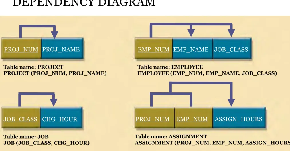
DEPENDENCY DIAGRAM
PROJ_NUM PROJ_NAME EMP_NUM EMP_NAME JOB_CLASS
Table name: PROJECT
PROJECT (PROJ_NUM, PROJ_NAME)
Table name: EMPLOYEE
EMPLOYEE (EMP_NUM, EMP_NAME, JOB_CLASS)
JOB_CLASS CHG_HOUR PROJ_NUM EMP_NUM ASSIGN_HOURS
Table name: JOB
JOB (JOB_CLASS, CHG_HOUR)
Table name: ASSIGNMENT
ASSIGNMENT (PROJ_NUM, EMP_NUM, ASSIGN_HOURS)
•
In other words, after the 3NF conversion has been completed,
your database will contain four tables:
PROJECT (PROJ_NUM
,
PROJ_NAME)
EMPLOYEE (EMP_NUM, EMP_NAME, JOB_CLASS)
JOB (JOB_CLASS, CHG_HOUR)
ASSIGNMENT (PROJ_NUM, EMP_NUM, ASSIGN_HOURS)
•
Note that this conversion has eliminated the original
EMPLOYEE table’s transitive dependency; the tables are now
said to be in third normal form (3NF).
3NF Definition
•
A table is in
third normal form (3NF)
when:
It is in 2NF
and
•
It is interesting to note the similarities between resolving 2NF
and 3NF problems.
•
To convert a table from 1NF to 2NF, it is necessary to remove
the partial dependencies. To convert a table from 2NF to 3NF,
it is necessary to remove the transitive dependencies.
•
No matter whether the “problem” dependency is a partial
dependency or a transitive dependency, the solution is the
same.
•
Create a new table for each problem dependency. The
determinant of the problem dependency remains in the
original table and is placed as the primary key of the new
table.
•
The dependents of the problem dependency are removed from
the original table and placed as nonprime attributes in the
new table.
Improving the design
•
The table structures are cleaned up to eliminate
the
troublesome
partial
and
transitive
dependencies.
•
You can now focus on improving the database’s
ability to provide information and on enhancing
its operational characteristics.
•
Remember that normalization cannot, by itself, be relied
on to make good designs.
•
Instead, normalization is valuable because its use helps
eliminate data redundancies.
•
There are various types of
issues
you need to address to
produce a good normalized set of tables:
1.
Evaluate PK assignments
2. Evaluate naming conventions
It is best to adhere to the naming conventions
3. Refine attribute atomicity
It is generally good practice to pay attention to the atomicity
requirement. An atomic attribute is one that cannot be further subdivided. Such an attribute is said to display
4. Identify new attributes
5. Identify new relationships
6. Refine primary keys as required for data granularity
Granularity
refers to the level of detail represented by
the values stored in a table’s row. Data stored at their
lowest level of granularity are said to be atomic data.
7. Maintain historical accuracy
8. Evaluate using derived attributes
•
The enhancements described are illustrated in the
tables and dependency diagrams shown in Fig. 5.7.
PROJ_NUM PROJ_NAME EMP_NUM JOB_CODE JOB_DESCRIPTION JOB_CHG_HOUR Table name: PROJECT Table name: JOB
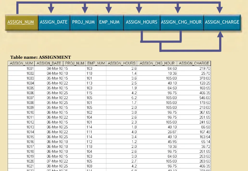
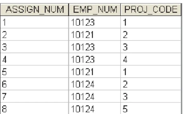
Table name: ASSIGNMENT
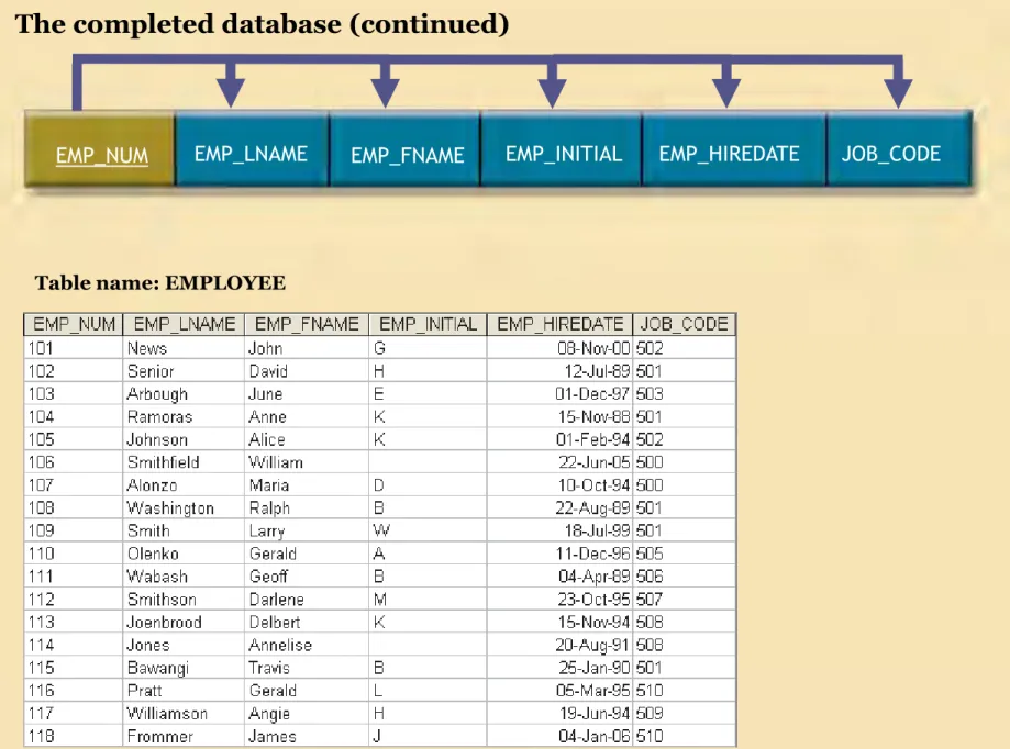
ASSIGN_NUM ASSIGN_DATE PROJ_NUM EMP_NUM ASSIGN_HOURS ASSIGN_CHG_HOUR ASSIGN_CHARGE The completed database (continued)
EMP_NUM EMP_LNAME EMP_FNAME EMP_INITIAL EMP_HIREDATE JOB_CODE
Table name: EMPLOYEE
Higher Level Normal Forms
• Tables in 3NF will perform suitably in business transactional databases. However, there are occasions when higher normal forms are useful.
• A table is in Boyce-Codd normal form (BCNF) when every determinant in the table is a candidate key.
• Recall from Module 3 that a candidate key has the same characteristics as a primary key, but for some reason, it was not chosen to be the primary key.
• Clearly, when a table contains only one candidate key, the 3NF and the BCNF are equivalent.
• Putting that proposition another way, BCNF can be violated only when the table contains more than one candidate key.
3NF, but not BCNF A B C D
A C B D
Partial dependency
1NF
A C D C B
3NF and BCNF 3NF and BCNF
Sample Data for BCNF Conversion
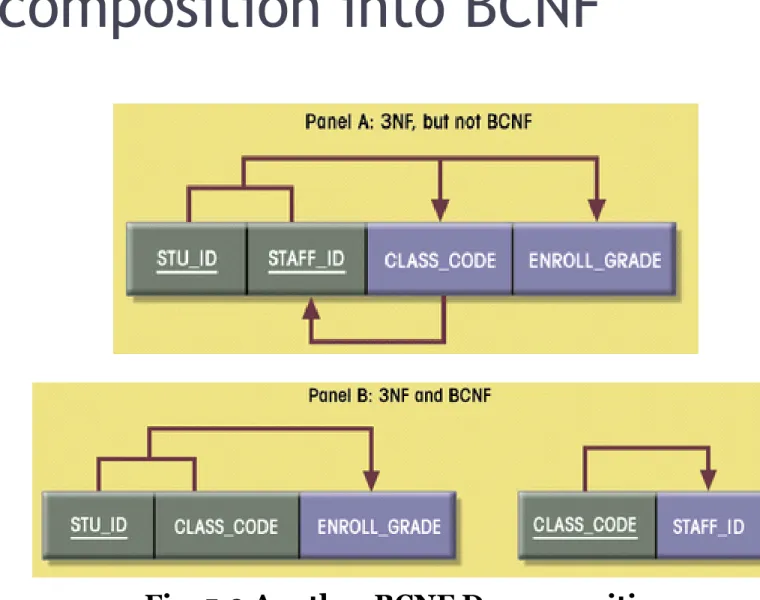
The structure shown in Table 5.2 is reflected in Panel A of Figure 5.9: STU_ID + STAFF_ID → CLASS_CODE, ENROLL_GRADE
CLASS_CODE → STAFF_ID
Panel A of Figure 5.9 shows a structure that is clearly in 3NF, but the table represented by this structure has a major problem, because it is trying to describe two things: staff assignments to classes and student enrollment information. Such a dual-purpose table structure will cause anomalies.
Decomposition into BCNF
BCNF Definition
Remember that a table is in BCNF when every
determinant in that table is a candidate key.
Therefore, when a table contains only one
candidate key, 3NF and BCNF are equivalent.
Fourth Normal Form (4NF)
•
You might encounter poorly designed databases, or
you might be asked to convert spreadsheets into a
database format in which multiple multivalued
attributes exist.
•
In normalization terminology, this situation is
referred to as a multivalued dependency.
•
A multivalued dependency occurs when one key
determines multiple values of two other attributes
and those attributes are independent of each other.
Table name: VOLUNTEER_V1
Table name: VOLUNTEER_V2
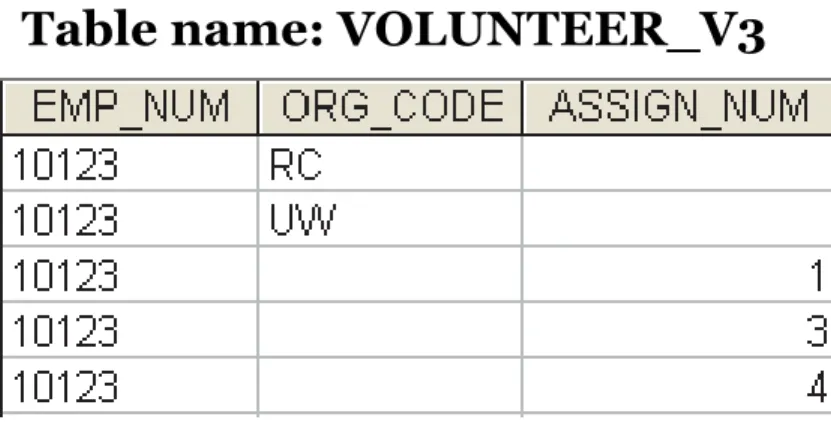
Table name: VOLUNTEER_V3
• One employee can have many service entries and many assignment entries.
• Therefore, one EMP_NUM can determine multiple values of ORG_CODE and multiple values of ASSIGN_NUM; however, ORG_CODE and ASSIGN_NUM are independent of each other.
• The presence of a multivalued dependency means that if versions 1 and 2 are implemented, the tables are likely to contain quite a few null values; in fact, the tables do not even have a viable candidate key.
• Such a condition is not desirable, especially when there are thousands of employees, many of whom may have multiple job assignments and many service activities.
• Version 3 at least has a PK, but it is composed of all of the attributes in the table. In fact, version 3 meets 3NF requirements, yet it contains many redundancies that are clearly undesirable.
•
The solution is to eliminate the problems caused by
the multivalued dependency. You do this by creating
new tables for the components of the multivalued
dependency.
•
In this example, the multivalued dependency is
resolved by creating the ASSIGNMENT and
SERVICE_V1 tables depicted in Figure 5.11.
•
Note that in Figure 5.11, neither the ASSIGNMENT
nor the SERVICE_V1 table contains a multivalued
dependency.
Fig. 5.11 A set of tables in 4NF
Table name: PROJECT
Table name: ASSIGNMENT
Table name: EMPLOYEE
Table name: ORGANIZATION
The relational diagram
4NF Definition
A table is in
fourth normal form (4NF)
when
it is in 3NF and has no multivalued dependencies.
Normalization and Database design
• Normalization should be part of the design process. Therefore, make sure that proposed entities meet the required normal form before the table structures are created.
• Keep in mind that if you follow the design procedures discussed in Module 3 and Module 4, the likelihood of data anomalies will be small.
• But even the best database designers are known to make occasional mistakes that come to light during normalization checks.
• However, many of the real-world databases you encounter will have been improperly designed or burdened with anomalies if they were improperly modified over the course of time. And that means you might be asked to redesign and modify existing databases that are, in effect, anomaly traps.
• Therefore, you should be aware of good design principles and procedures as well as normalization procedures.
•
First, an ERD is created through an iterative process.
▫ You begin by identifying relevant entities, their attributes,
and their relationships. Then you use the results to identify
additional entities and attributes.
▫ The ERD provides the big picture, or macro view, of an
organization’s data requirements and operations.
•
Second, normalization focuses on the characteristics of
specific entities; that is, normalization represents a
micro view of the entities within the ERD.
•
It is difficult to separate the normalization process from
the ER modeling process; the two techniques are used in
an iterative and incremental process.
Denormalization
• It’s important to remember that the optimal relational database implementation requires that all tables be at least in third normal form (3NF).
• A good relational DBMS excels at managing normalized relations; that is, relations void of any unnecessary redundancies that might cause data anomalies.
• Although the creation of normalized relations is an important database design goal, it is only one of many such goals. Good database design also considers processing (or reporting) requirements and processing speed.
• The problem with normalization is that as tables are decomposed to conform to normalization requirements, the number of database tables expands. Therefore, in order to generate information, data must be put together from various tables. Joining a large number of tables takes additional input/output (I/O) operations and processing logic, thereby reducing system speed.
• Most relational database systems are able to handle joins very efficiently. However, rare and occasional circumstances may allow some degree of denormalization so processing speed can be increased.
Common Denormalization Examples
CASE EXAMPLE RATIONALE and CONTROLS
Redundant data
Storing ZIP and CITY attributes in the CUSTOMER table when ZIP determines CITY
• Avoid extra joint operations.
• Program can validate city (drop-down box) based on the zip code.
Derived data Storing STU_HRS and STU_CLASS (student classification) when
STU_HRS determines STU_CLASS.
• Avoid extra joint operations.
• Program can validate classification (lookup) based on the student
hours. Preaggregated
data (also derived data)
Storing the student grade point average (STU_GPA) aggregate value in the STUDENT table when this can be calculated from the ENROLL and COURSE tables.
• Avoid extra joint operations.
• Program computes the GPA every time a grade is entered or updated.
• STU_GPA can be updated only via administrative routine.
Information requirements
Using a temporary denormalized table to hold report data. This is required when creating a tabular report in which the columns represent data that are stored in the table as rows.
• Impossible to generate the data
required by the report using plain SQL. • No need to maintain table. Temporary table is deleted once report is done.
Denormalization
•
Normalization is only one of many database design
goals.
•
Normalized (decomposed) tables require additional
processing, reducing system speed.
•
Normalization purity is often difficult to sustain in
the modern database environment.
•
The conflict between design efficiency, information
requirements, and processing speed are often
resolved
through
compromises
that
include
denormalization.
BUSINESS RULES
• Properly document and verify all business rules with the end users.
• Ensure that all business rules are written precisely, clearly, and simply. The business rules must help identify entities, attributes, relationships, and constraints.
• Identify the source of all business rules, and ensure that each business rule is justified, dated, and signed off by an approving authority.
DATA MODELING
Naming Conventions: All names should be limited in length (database-dependent size).
• Entity Names:
• Should be nouns that are familiar to business and should be short and meaningful
• Should document abbreviations, synonyms, and aliases for each entity
• Should be unique within the model
• For composite entities, may include a combination of abbreviated names of the entities linked through the composite entity
•
Attribute Names:
▫ Should be unique within the entity
▫ Should use the entity abbreviation as a prefix
▫ Should be descriptive of the characteristic
▫ Should use suffixes such as _ID, _NUM, or
_CODE for the PK attribute
▫ Should not be a reserved word
▫ Should not contain spaces or special characters
such as @, !, or &
•
Relationship Names:
▫ Should be active or passive verbs that clearly
indicate the nature of the relationship
Entities:
▫ Each entity should represent a single subject.
▫ Each entity should represent a set of distinguishable entity instances.
▫ All entities should be in 3NF or higher. Any entities below 3NF should be justified.
▫ The granularity of the entity instance should be clearly defined. ▫ The PK should be clearly defined and support the selected data
granularity.
Attributes:
▫ Should be simple and single-valued (atomic data)
▫ Should document default values, constraints, synonyms, and aliases
▫ Derived attributes should be clearly identified and include source(s)
▫ Should not be redundant unless this is required for transaction accuracy, performance, or maintaining a history
Relationships:
▫ Should clearly identify relationship participants
▫ Should clearly define participation, connectivity, and
document cardinality
ER Model:
▫ Should be validated against expected processes:
inserts, updates, and deletes
▫ Should evaluate where, when, and how to maintain a
history
▫ Should not contain redundant relationships except as
required (see attributes)
▫ Should minimize data redundancy to ensure
single-place updates
▫ Should conform to the minimal data rule: “All that is
needed is there, and all that is there is needed.”
Summary of Module 5
•
Normalization is a technique used to design tables
in which data redundancies are minimized.
•
The first three normal forms (1NF, 2NF, and 3NF)
are most commonly encountered. From a structural
point of view, higher normal forms are better than
lower normal forms, because higher normal forms
yield relatively fewer data redundancies in the
database.
•
Almost all business designs use 3NF as the ideal
normal form. A special, more restricted 3NF known
as Boyce-Codd normal form, or BCNF, is also used.
• A table is in 1NF when all key attributes are defined and when all remaining attributes are dependent on the primary key. However, a table in 1NF can still contain both partial and transitive dependencies. (A partial dependency is one in which an attribute is functionally dependent on only a part of a multiattribute primary key. A transitive dependency is one in which one attribute is functionally dependent on another nonkey attribute.) A table with a single-attribute primary key cannot exhibit partial dependencies.
• A table is in 2NF when it is in 1NF and contains no partial dependencies. Therefore, a 1NF table is automatically in 2NF when its primary key is based on only a single attribute. A table in 2NF may still contain transitive dependencies.
• A table is in 3NF when it is in 2NF and contains no transitive dependencies. Given that definition of 3NF, the Boyce-Codd normal form (BCNF) is merely a special 3NF case in which all determinant keys are candidate keys. When a table has only a single candidate key, a 3NF table is automatically in BCNF.
• A table that is not in 3NF may be split into new tables until all of the tables meet the 3NF requirements.
• Normalization is an important part—but only a part—of the design process. As entities and attributes are defined during the ER modeling process, subject each entity (set) to normalization checks and form new entity (sets) as required. Incorporate the normalized entities into the ERD and continue the iterative ER process until all entities and their attributes are defined and all equivalent tables are in 3NF.
• A table in 3NF might contain multivalued dependencies that produce either numerous null values or redundant data. Therefore, it might be necessary to convert a 3NF table to the fourth normal form (4NF) by splitting the table to remove the multivalued dependencies. Thus, a table is in 4NF when it is in 3NF and contains no multivalued dependencies.
• The larger the number of tables, the more additional I/O operations and processing logic required to join them. Therefore, tables are sometimes denormalized to yield less I/O in order to increase processing speed. Unfortunately, with larger tables, you pay for the increased processing speed by making the data updates less efficient, by making indexing more cumbersome, and by introducing data redundancies that are likely to yield data anomalies. In the design of production databases, use denormalization sparingly and cautiously.
• The Data-Modeling Checklist provides a way for the designer to check that the ERD meets a set of minimum requirements.