LOGISTIC APPROXIMATIONS OF MARGINAL TRACE LINES FOR BIFACTOR ITEM RESPONSE THEORY MODELS
Brian Dale Stucky
A dissertation submitted to the faculty of the University of North Carolina at Chapel Hill in partial fulfillment of the requirements for the degree of Doctor of Philosophy in the
Department of Psychology (Quantitative).
Chapel Hill 2011
ABSTRACT
BRIAN STUCKY: Logistic Approximations of Marginal Trace Lines for Bifactor Item Response Theory Models
(Under the direction of David Thissen, Ph.D.)
Bifactor item response theory models are useful when item responses are best represented by a general, or primary, dimension and one or more secondary dimensions that account for relationships among subsets of items. Understanding slope parameter estimates in multidimensional item response theory models is often challenging because interpretation of a given slope parameter must be made conditional on the item’s other parameters. The present work provides a method of computing marginal trace lines for an item loading on more than one dimension. The marginal trace line provides the relationship between the item response and the primary dimension, after accounting for all other dimensions. Findings suggest that a logistic function, common in many applications of item response theory, closely approximates the marginal trace line in a variety of model related conditions.
Additionally, a method of IRT-based scoring is proposed that uses the logistic approximation marginal trace lines in a unidimensional fashion to compute scaled scores and standard deviation estimates for the primary dimension.
The utility of the logistic approximation for marginal trace lines is considered across a wide range of varying bifactor parameter estimates, and under each condition the marginal is closely approximated by a logistic function. In addition, it is shown that use of the logistic approximations to conduct item response theory-based scoring should be restricted to
dependence. Under this restriction, scaled scores and posterior standard deviations are nearly equivalent to other MIRT-based scoring procedures. Finally, a real-data application is
provided which illustrates the utility of logistic approximations of marginal trace lines in item selection and scale development scenarios.
ACKNOWLEDGEMENTS
I am indebted to my adviser Dr. David Thissen, and the faculty and students of the L.L. Thurstone Psychometric Laboratory. I also wish to thank Randy Schuler.
TABLE OF CONTENTS
LIST OF TABLES...vii
LIST OF FIGURES...viii
Chapter I. AN OVERVIEW OF MULTIDIMENSIONAL ITEM RESPONSE THEORY...1
The effects of ignoring local dependence...2
Compensatory MIRT models...…...4
MIRT scoring……….…...7
Bifactor models….……….…...10
Depressive symptoms example…………..……...14
II. COMPUTING AND APPROXIMATING MARGINAL TRACE LINES………17
Logistic approximations……….……....20
The logistic as a close approximation of the marginal trace line...22
The relation between conditional and marginal slope parameters...27
III. COMPUTING ITEM RESPONSE THEORY SCORES FROM MARGINAL TRACE LINES...31
An overview of IRT-scaled scores for response patterns and summed scores...32
The method of evaluating primary dimension scores across MIRT models...35
An IRT-based scoring example...38
Controlling local dependence...…………....……46
Scoring results………...………...……..49
Summary of findings: Ignoring local dependence.………..………...58
Summary of findings: Controlling for local dependence.…...59
IV. AN APPLICATION OF MARGINAL TRACE LINES FOR BIFACTOR ITEM RESPONSE THEORY MODELS...65
Re-evaluating an asthma symptoms scale...66
Comparing the logistic approximation and two-tier algorithm...78
V. CONCLUSIONS……...80
APPENDIX I...82
REFERENCES...84
LIST OF TABLES Table
1. Example of bifactor structure...11 2. Example of modified-bifactor structure...12 3. Unidimensional and bifactor slope parameters for
eight depressive symptoms items...15 4. Four 2-PL MIRT models and corresponding marginal parameter estimates….…...24 5. Example of bifactor structure for scoring...39 6. Example of a score translation table using the logistic approximation of
marginal trace lines and the two-tier algorithm...40 7. Maximum difference in EAPs between tests scored with the two-tier
algorithm and the logistic approximation of the marginal trace line...….61 8. Maximum difference in score SDs between tests scored with the two-tier
algorithm and the logistic approximation of the marginal trace ...…….….…63 9. A comparison of conditional and marginal slope parameters
for 33 asthma symptoms items………....…68 10.A comparison of conditional, marginal, and univariate slope parameters
for 33 asthma symptoms items……….…...…72 11.A comparison of marginal and univariate thresholds for the
reduced 18-item scale………..…...…73 12.Marginal/Conditional and Univariate EAPs and SDs for
18 asthma symptoms items………...76
viii
LIST OF FIGURES Figure
1. Trace surface for an item more discriminating on the primary dimension……...6
2. Multivariate posterior density for a correct response to an item discriminating on two dimensions……….……..9
3. θ1 trace lines conditional on θ2...13
4. Marginal and conditional trace lines...19
5. Four 2-PL marginal trace lines and logistic approximations...25
6. Four 2-PL marginal trace lines and logistic approximations in log odds...26
7. Marginal slopes for items with equal conditional slopes on two dimensions...27
8. Marginal slopes across a range of conditional slopes on two dimensions...30
9. Long scale, six clusters (λP = 0.5 – 0.7, λS = 0.3 – 0.5)...42
10.Medium scale, three doublets (λP = 0.5 – 0.7, λS = 0.3 – 0.5)...43
11.Short scale, one doublet (λP = 0.7 – 0.9, λS = 0.5 – 0.7)...44
12.Including all items and using locally independent items only: Long scale, six clusters (λP = 0.5 – 0.7, λS = 0.3 – 0.5)...51
13.Including all items and using locally independent items only: Medium scale, three doublets (λP = 0.5 – 0.7, λS = 0.3 – 0.5)...52
14.Including all items and using locally independent items only: Short scale, one doublet (λP = 0.7 – 0.9, λS = 0.5 – 0.7)...53
15.Including all items and using locally independent items only: Medium scale, three doublets (λP = 0.7 – 0.9, λS = 0.5 – 0.7)...54
16.Including all items and using locally independent items only: Long scale, six clusters (λP = 0.7 – 0.9, λS = 0.5 – 0.7)...55
CHAPTER 1
AN OVERVIEW OF MULTIDIMENSIONAL ITEM RESPONSE THEORY Item response theory (IRT) is a useful technique for item analysis and scoring which is becoming increasingly common in educational measurement, health outcomes research, and psychology. IRT models propose that the probability of response to an item is a function of the characteristics of the item (i.e., item parameters) and the individual’s location on the latent trait(s) (i.e., person parameters). This item response function, or trace line, conveys all information available from the item that can be used to estimate an individual’s latent trait. When used in combination with multiple items, the trace lines form the likelihood, from which one can determine the location on the latent variable where the trait level is most likely.
IRT score estimates may be computed for either unidimensional (UIRT) or multidimensional (MIRT) models. UIRT scores are appropriate when the relationships among the items, given an individual’s trait level, can be accounted for by a single latent variable. When no additional latent variables are needed to account for response covariation beyond the single dimension, the item set satisfies the assumptions of unidimensionality and local independence. However, if fitting the item response data requires multiple latent variables, then MIRT models are needed to achieve local independence.
these situations it is often useful to account for LD among a subset of items by estimating an additional latent variable (e.g., in a bifactor model). As a special class of MIRT models, bifactor models account for the shared relations among all the items through a general, or primary, dimension and one or more secondary dimensions, orthogonal to the primary dimension, which contain loadings only for those locally dependent items.
Traditionally, bifactor models have been employed only to identify LD (i.e., multidimensionality). In order to provide unidimensional scores for such models, the most common approach has been to set items aside from secondary dimensions, eliminating the dependence, and then to use the remaining items to compute scores with a unidimensional model. The present research aims to develop a method in which violations of
unidimensionality can be accounted for in a bifactor model while still producing
unidimensional scores. In other words, the model is allowed the flexibility to account for multiple dimensions, while the scores reflect the individual’s location on the general factor.
The Effects of Ignoring Local Dependence
When a set of items is best represented by a single dimension it is referred to as unidimensional. Unidimensionality implies local independence, which indicates that all the relationships among the data are accounted for by the underlying latent variable. Consider a pair of items i and j with trace lines Ti and Tj which “trace” the probability of response given the latent variable (θ). If the response model is defined by a single dimension, then the probability of an individual correctly responding to both items is equal to the product of the individual trace lines given the latent variable:
T u( i =1,uj =1| )θ =T u( i =1| ) (θ T uj =1|θ). (1)
In other words, if local independence holds, then the joint likelihood of a particular response pattern is properly represented by the product of the separate probabilities of item responses. Of course, this should also hold for all the items in a test conditional on θ.
In the 1980’s, prior to usable implementations of MIRT models, researchers struggled to determine how robust IRT models were to violations of unidimensionality. The majority of this work involved generating multidimensional data from simple structure factor analysis models with varying degrees of correlation between factors, and then comparing parameter and individual trait estimates after fitting UIRT models. To briefly summarize, numerous authors suggest that when separate dimensions are correlated greater than about r = .60, a single factor may adequately represent the factor structure (Folk & Green, 1989; Drasgow & Parsons, 1983; Ackerman, 1989; Harrison, 1986; Reckase, 1979). Additionally, trait
recovery is improved when the general factor is strongly unidimensional and contains a large number of items with a high degree of information (Harrison, 1986).
Though prior research attempted to validate the use of fitting UIRT models to
multidimensional data, the costs can be great, including “θ-theft” (i.e., when a small number of locally dependent items define the dimension; Thissen & Steinberg, 2010, p. 131), over-estimating score reliability (Thissen, Steinberg, & Mooney, 1989), and in misrepresenting the data. In practice θ-estimates often give the appearance of robustness to violations of
unidimensionality, or as Demars (2006) says, “if the focus is on estimated theta and not the item parameters, any of the models will perform satisfactorily…” (p. 165). Importantly, it is the factor structure, or item parameter interpretations, that are most often misrepresented in unidimensional representations of multidimensional data. So, while differences in score
precision may be appear slight, interpretation of the latent trait based on the dimensions’ parameters is often what is most affected.
Much of the past research on the robustness of UIRT models to violations of local independence was conducted prior to the availability of usable implementations of MIRT models. Hence, previous research was motivated in large part by a desire to fit UIRT models, because MIRT models were not a viable alternative. Past investigations, though important in understanding under what conditions essential unidimensionality may be sufficient, are of less relevance now that well established procedures are in place for fitting MIRT models (Reckase, 2009).
Compensatory MIRT Models
When fitting item responses requires more than one latent trait, MIRT models may be appropriate (McKinley & Reckase, 1983; Reckase, 1985). The most widely used are
compensatory1 MIRT models, which model the probability of a response with a linear combination of latent variables (θ-coordinates). In other words, if an individual’s location is low on a particular trait, the linear combination may compensate with a high score on another trait.
For simplicity, consider the 2PL compensatory MIRT model as an extension of the 2PL univariate IRT model (for multivariate extensions of Samejima’s (1969) graded
response model see Muraki and Carlson (1993)). The probability of a person with trait vector
θ responding correctly to item i is based on a vector of discrimination parameters ai and an intercept ci:
1 Other, less often used MIRT models are noncompensatory (Sympson, 1978). This class of models
can be considered the combination of separate unidimensional models. Here the probability of correct response for an item is often formed from the product of the separate probabilities for the latent traits. The models are said to be noncompensatory because the probability of correct response cannot be higher than any of the probabilities in the product.
( 1| , , ) 1
i i
i i
c
i ij j i i c
e
T u c
e
+ +
= =
+
aθ
aθ
θ a .
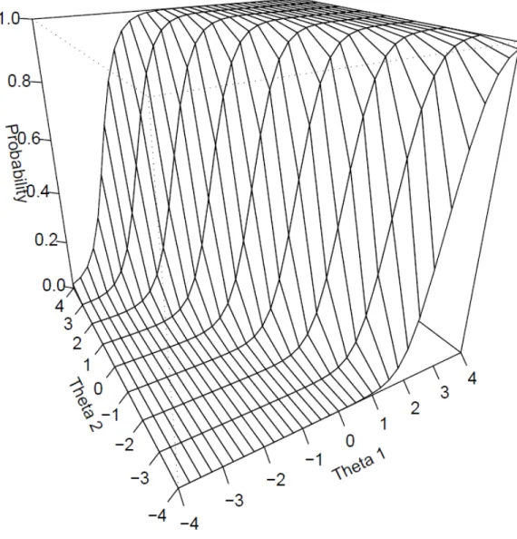
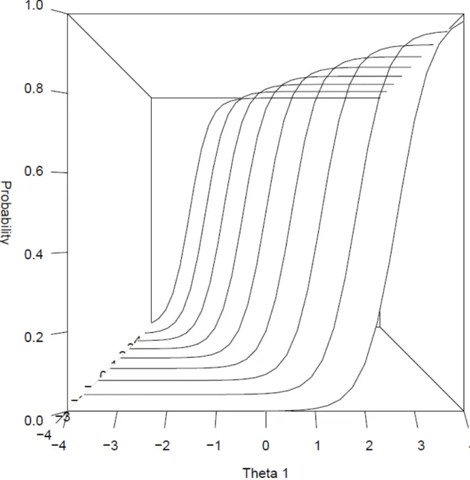
(2) Unlike the difficulty parameter in the UIRT 2PL model, ci represents the relative difficulty of an item without respect to a trait dimension. Because more than one dimension affects responses, graphical representations (trace surfaces) are often used to depict the relation between item responses along 2-dimensions. Figure 1 illustrates the trace surface for an item with a1 = 3, a2 = 2, c = 0.
Figure 1. Trace surface for an item more discriminating on the primary dimension
That the probability of a correct response increases more rapidly along θ1 indicates
that the first dimension has a greater effect on responses for this item. The compensatory nature of the model is also evident. The exponent in eq. 2 is a linear combination of θ and a -vectors with an intercept c. If the exponent is equal to 0, then eq. 2 simplifies to Ti = ½ because e0 = 1. Rearranging the terms in the exponent then provides the line through the θ -space where the probability of correct response is 0.5:
2 1 1
2
1 (a a
θ = − θ −c) 3)
ce, for the present example, relatively low trait levels on θ1 (say θ1 = -2) can be
tem r
MIRT Scoring
The relative utility of MIRT mo ged by the scores they produce. In general
. (
Hen
compensated for by high levels of θ2 (i.e., θ2 = 3). Note that because this particular i
better discriminates on the θ1 dimension, higher levels of θ2 are required to compensate fo
low levels of trait θ1.
dels may be jud
, MIRT scores may be thought of as a multivariate extension of UIRT scoring. The likelihood of a particular response pattern is computed by the following:
, n 1 ( | ) ( ) i u i
L T
θ
= =
∏
U θ
(4)
where L ponse pattern to a n it
all (U|θ) is the likelihood of a res em test for an individual with response pattern U = {u1, u2,…, un} (Segall, 1996). For certain extreme response patterns, correct (or positive) or incorrect (or negative) responses to test items (which are common in short tests), the mean of the likelihood becomes undefined, the mode is infinite, and some heuristic is needed to compute scores. For this and other reasons, it is useful to employ a
prior distribution and obtain posteriors for response patterns. In the multivariate case, the posterior function takes the form,
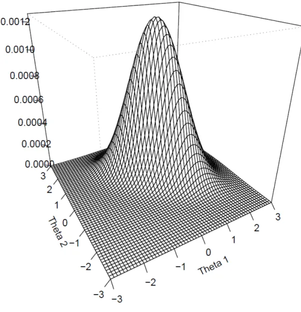
f( | )θ U =L( | ) ( ),U θ φ θ (5) where the posterior f(θ|U) is the product of the response pattern likelihood L(U|θ) and φf(θ), the multivariate normal distribution of θ.2 Using the parameters from Figure 1, Figure 2 displays the posterior density for a correct item response.
2When the model takes on an oblique simple structure form, the multivariate normal distribution has
a mean vector of zeros and a variance-covariance matrix Φ with 1 along the diagonal elements and the population based covariances of the dimensions on the off-diagonal elements. In the case where the dimensions are correlated 1.0, and simple structure is imposed, the posterior equation reduces to the unidimensional case.
Figure 2. Multivariate posterior density for a correct response to an item discriminating on two dimensions
The mode of the posterior density in Figure 2 provides the most likely trait estimate based on a correct response and the normal distribution (Maximum A Posteriori, MAP); the mean of that density is the two-dimensional Expected A Posteriori (EAP).
The only reasonable advantage to using a MIRT-, rather than UIRT-based scoring procedure, is if the scores MIRT models produce have large enough gains in reliability to
warrant the added complexity of the model. Theoretically, so long as the dimensions of a test are correlated, MIRT scores should have greater precision than UIRT scores. This is because of what Segall (2000) refers to as “cross-information”- that scores on one dimension inform scores on another dimension. In other words, if dimensions are correlated, then a high score on one dimension is expected to correspond with a high-score on another dimension. The effect of this additional information is either increased score precision or reduced test length. However, the actual increases in reliability due to MIRT are considered marginal (from about .1 to negligible (Segall, 1996; Luecht, 1996)). It may be that gains are most substantial for domains that begin with relatively low levels of information, but are highly correlated with some other more precisely measured domain (requiring correlations perhaps greater than .6).
When faced with strongly correlated dimensions, researchers are presented with a number of alternatives. If the potential dimensions are weakly correlated, then little is gained from the MIRT model and fitting multiple UIRT models seems a better option. If the
dimensions are highly correlated, then some degree of score precision is gained through the MIRT model, but perhaps at the cost of scores with complex interpretations. With highly correlated domains there exists the possibility of a general factor which underlies the items, along with some number of group-specific factors which account for variance particular to only subsets of items.
Bifactor Models
Bifactor models (Holzinger & Swineford, 1937; Tucker, 1958; Gibbons & Hedeker, 1992) are used in situations in which a set of items may be represented by a general (or primary) latent variable in addition to a number of secondary dimensions (or group or content factors) which account for covariance specific to subsets of items. The utility of bifactor
models lies in their broad range of application: Bifactor models are useful when multiple dimensions are expected, or when multidimensionality is caused by unwanted local dependence among item subsets.
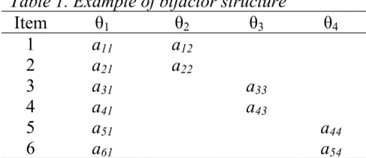
Gibbons and Hedeker (1992) describe the bifactor structure in which all items receive one slope parameter on the general dimension and one slope parameter on a secondary dimension (see Table 1). This structure is imposed a priori by researchers in situations in which a single dimension is hypothesized to underlie all items on a scale, but additional dimensions are require to account for covariation specific to subsets of items. For example, bifactor models have been used in psychological studies aimed at understanding inter-related but distinct concepts including, but not limited to, depression, anxiety, and anger (e.g., Simms, Gros, Watson, & O’Hara, 2008; Irwin, et al., 2010). In this framework, each concept is represented by a content-specific subfactor, and the primary dimension may be described as general distress/dysphoria. In educational settings, the bifactor model is often used in tests of reading comprehension, where reading passages are followed by a set of related items. The general factor of the bifactor model is reading comprehensions, and additional specific-factors are required for items belonging to each passage.
Table 1. Example of bifactor structure
Item θ1 θ2 θ3 θ4
1 a11 a12
2 a21 a22
3 a31 a33
4 a41 a43
5 a51 a44
6 a61 a54
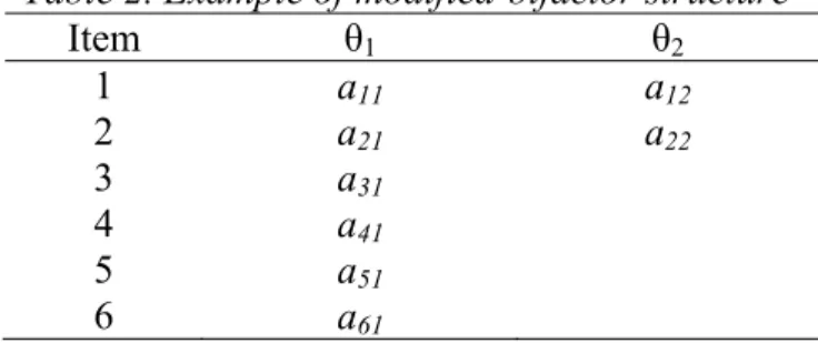
Alternatively, when bifactor models are employed to account for undesired local dependence, a modification to the bifactor structure is made in which only locally dependent subsets of items receive the additional specific-factor loading (Table 2). These models are
appropriate in situations in which a single latent variable is hypothesized, but subsequent analyses reveal the presence of unaccounted relationships among subsets of test items. In such situations local independence may be achieved by modeling the additional relationships with one or more sub-factors. The following section provides an example of modeling nuisance local dependence in a set of depression items with a modified-bifactor model.
Table 2. Example of modified-bifactor structure
Item θ1 θ2
1 a11 a12
2 a21 a22
3 a31
4 a41
5 a51
6 a61
Both the bifactor and modified-bifactor models serve as an indication of the
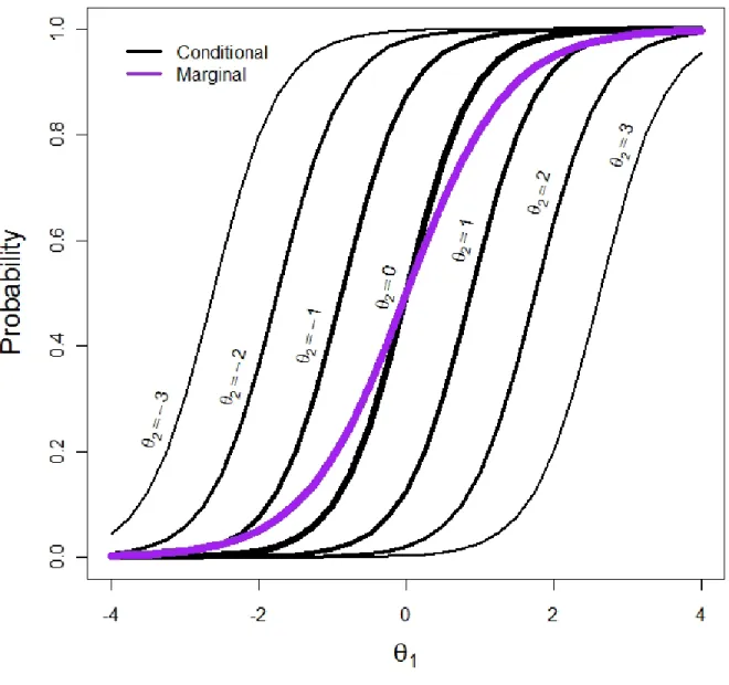
dimensionality of a collection of items. In assessing dimensionality, interpretation is focused on the model’s slope parameters. Specifically, the magnitude of the secondary dimension slope parameter indicates the influence of this dimension in accounting for relations among responses, but the ratio between general and secondary dimension slopes also indicate the relative strength of each factor. However, interpreting the model in this manner remains limited to assessing the probability of response on one dimension conditional on the model’s other dimension(s). Figure 3 illustrates this concept. Using the same parameter estimates as Figure 1 (a1 = 3, a2 = 2, c = 0), the trace surface is now viewed along the θ1 dimension and the θ2 slopes have been removed. What remains are the item’s θ1 trace lines conditional on varying locations of θ2.
Figure 3. θ1 trace lines conditional on θ2
In other words, a slope on θ1 (or the general factor in the bifactor case) does not
indicate the marginal relation between an item response and θ1, but rather the relation
between an item response on θ1 at various locations on θ2. Because of this, in bifactor
models the primary dimension slope interpretation may be confused or misleading.
Depressive Symptoms Example
To illustrate the difficulties in interpreting bifactor item parameters, considered below are a series of analyses conducted on an eight-item subset of the Patient Reported Outcomes Measurement Information System (PROMIS) pediatric Depressive Symptoms scale (Irwin, et al. 2010). The original 14-item scale was developed from 22 tryout items administered to at least 759 youth aged 12-17 in hospital clinics in North Carolina and Texas. For the purpose of this illustration, eight items were selected to be re-analyzed as a separate scale (the eight items may be found in Table 3). Six of the eight items were from the scale as ultimately assembled and published (Irwin, et al. 2010), and the two additional items were from a locally dependent pair of items identified and set aside during the item tryout period. Specifically, in the analyses reported by Irwin et al. (2010), the items “I cried more than usual” and “I felt like crying” were modeled with a residual correlation in a factor analytic framework.
In this illustration, we fit unidimensional IRT and bifactor MIRT models to the eight-item subset. Table 3 provides the results of fitting two separate models. The first model assumes unidimensionality, while the second bifactor model estimates a general dimension and a secondary dimension for the two locally dependent items with equality constraints on the slope parameters. Comparing the slope parameters on the six unidimensional items between the unidimensional IRT model and bifactor MIRT model indicates that the slope parameters differ little (less than 0.1). However, for the two locally dependent “crying” items, the slope parameters on the primary dimension substantially increase in comparison to the unidimensional estimate (more than 0.4). This effect occurs for any bifactor model in which the slopes on the secondary dimensions are non-zero. The compensatory nature of
model accounts for item responses based on the total number of dimensions present. For items with slopes constrained to zero for the secondary dimension, the interpretation is consistent with the unidimensional model, and any difference in slopes may be due to the additional variance accounted for by the secondary dimensions3. However, for items with non-zero slopes on more than one dimension, the interpretation of the primary dimension slope must be made conditional on the secondary dimension slope. In other words, it would be incorrect to interpret the primary dimension slope, for an item with more than one slope, as one would a univariate slope parameter. It may then be desirable to obtain the marginal
relation between the item response and primary dimension that averages over the secondary dimension(s).
Table 3. Unidimensional and bifactor slope parameters for eight depressive symptoms items.
UIRT MIRT
Item a aPrimary aSubfactor
I cried more than usual. 1.78 2.22 1.94
I felt like crying. 1.79 2.33 1.94
I felt everything in my life went wrong. 2.39 2.49 ---- I felt like I couldn't do anything right. 2.31 2.45 ----
I felt alone 2.20 2.12 ----
I felt so bad that I didn’t want to do anything. 1.93 1.98 ---- Being sad made it hard for me to do things with
my friends. 1.92 1.94 ----
I wanted to be by myself. 0.73 0.75 ----
Note: Items in italics have been previously identified as locally dependent (Irwin et al., 2010).
This dissertation develops a technique for computing the marginal, or average, trace line for the primary dimension after accounting for secondary dimensions in bifactor models and assesses the appropriateness of a logistic approximation (Chapter 2). Next, the
3 In this example, the difference in slopes for the six unidimensional items suggests that the two
locally dependent “crying” items have re-oriented the latent variable in the unidimensional model. When the dependence between the “crying” items is accounted for, the slopes on the primary
dimension slightly increase for the six items, indicating primary dimension is less influenced by local dependence.
16
technique is used to compute IRT-based primary dimension scale score estimates and
CHAPTER 2
COMPUTING AND APPROXIMATING MARGINAL TRACE LINES In a 2-dimensional MIRT model, to obtain the marginal trace line for θ1, one must
average over the θ2 dimension of the multivariate trace surface:
TMarginali(ui =1|θ1)=
∫
Ti(θ1,θ2)φ(θ2)dθ2. ( In th6) is 2-dimensional example, the product of the θ1 conditional trace lines from the trace
e
itional
e univariate trace line in
unidim f
for
ore
surface, Ti(θ1,θ2) and the univariate normal distribution, integrated across θ2, represents th
marginal trace line for θ1, TMarginal. Note that (6) is essentially computing the marginal trace
line by weighting the θ1 conditional trace lines by the normal distribution. Because of this
weighting process, marginal trace lines will never be greater in magnitude than the conditional trace lines along θ1, and depending on the relationship between the cond slopes (a1 and a2) the marginal slope may be much smaller.
Interpretation of the marginal trace line is not unlike th
ensional IRT; the marginal trace line is the relationship between the probability o response given θ1, after accounting for the secondary dimension(s).4 Using the parameters
the first item in the depressive symptoms example in Chapter 1, I cried more than usual, one may illustrate this phenomenon by considering the θ1 marginal (6) and conditional trace lines
(2) at various locations on θ2 (Figure 4). The varying degrees of line width are meant to
suggest that conditional trace lines closer to the mean of the normal distribution receive m
weight than those near the tails of the distribution. Clearly the slope of the marginal trace line is less than that of the conditional trace lines. Recall that a1 for the item I cried more
than usual was 2.22, but after computing the marginal, aMarginal is reduced to 1.46. As
researchers interpret such parameter estimates, the (conditional) slopes on the general dimension may be misleading as they suggest a relationship which is in fact inflated du the secondary dimension. After accounting for the secondary dimension, the marginal trace line gives a more realistic account of the relationship between the item and general factor.
e to
Figure 4. Marginal and conditional trace lines
Figure 4 also illustrates the curious fact that when item calibration moves from a unidimensional model to a bifactor model, slope parameters on the factor of interest tend to increase, giving the false impression that items are more representative of the general factor. Rather, in keeping with prior literature (Reckase, 1979), one might expect that unmodeled LD should produce over-estimates of slope parameters on the on the unidimensional factor (i.e., “θ theft”; Thissen and Steinberg, 2010), and that after accounting for LD, slopes on the
general dimension should decrease. This surprising phenomenon is again attributable to slopes in bifactor models being conditional, rather than marginal, representations of item responses; when the marginal trace line is computed (as in Figure 4), the slope parameter takes on a more realistic value.
Logistic Approximations
Note that thus far the marginal trace line has been derived from a MIRT model, but has no item parameters which describe the relationship between the item and marginal θ1
distribution. The expected score curve from a multidimensional logistic trace surface with a normal population distribution is not a logistic function or, indeed, any “simple” function. The marginal trace line may be thought of as an average of the θ1 conditional trace lines
weighted by the normal distribution, and a logistic approximation of this average trace line may suffice.
There is historical precedent for treating the summation of logistic functions as approximately logistic. Winsor (1932) notes that the “sum of a number of logistics does in fact often approximate closely a logistic as has been shown by Reed and Pearl (1927)” (p. 4). Reed and Pearl (1927) use sums of logistics to describe population growth, and later, Merrell (1931) would examine averages of individual growth curves to describe change over time for groups of individuals. From this perspective, one should expect that the marginal trace line, which is itself a weighted average of logistic curves, should be closely approximated by a logistic function.
Given the marginal trace line, to find a logistic approximation, one must estimate item parameters. A potential approximation to be considered involves computing the derivative of the marginal trace line at T = 0.5, which is an estimate of the slope of an
approximately logistic function. We may approximate the derivative by taking values of
Tmarginal and θ1 near T = 0.5:
log log 1 1 , H L H L H L T T T a θ θ − − − = −
) T (7)
where TH represents a probability slightly higher than 0.5, TL a probability slightly lower than 0.5, and θH and θL the respective θ1 trait values. The ratio between the difference in the log odds of two probabilities near 0.5 and their respective θ1 values gives the slope of the function or the marginal trace line . Next, the threshold or difficulty parameter is the location on θ1 where TMarginal is 0.5, and in practice is computed directly from the dimension
of interest in the MIRT model. For example, in a MIRT model where the marginal is desired for θ1, the threshold is:
i aˆ 1 ˆ i i i c b a −
= (8)
We may then approximate the marginal trace line using the traditional unidimensional logistic function and and (Birnbaum, 1968). In practice, the parameters computed from the numerical derivative tend to be sensitive to the number of quadrature points
provided. Because of this concern, an alternative method is used as originally proposed by Ip (2010a; 2010b).
ˆ
a bˆ aˆ
Ip’s method of approximation is equivalent to transforming the MIRT slope parameters into the factor analytic loading metric, and then back-translating to arrive at the marginal slopes. Ip’s method is equivalent to computing the marginal factor loading for the dimension of interest, in this case θ1:
(
)
, 1 2 1 Marginal∑
+ = D a D aλ (9)
where D is the commonly used scaling constant 1.7. The item variance unexplained by the primary latent dimension is then:
2 , (10)
Marginal 2
Marginal 1 λ
σ = −
and the marginal slope parameter is simply:
a D ⎟⎟ ⎟ ⎠ ⎞ ⎜⎜ ⎜ ⎝ ⎛ = 2 Maginal Marginal ˆ σ λ
. (11)
As with the numerical derivative, is unchanged after computing the marginal. A logistic approximation of the marginal trace line uses and in the traditional fashion of the 2-parameter logistic model:
ˆ b
ˆ
a bˆ
(
)
)] ˆ ( ˆ exp[ 1 1 | 1 1 1 i i i b a u T − − + = = θθ . (12)
Extensions to the graded response model (GRM; Samejima, 1969) provide no additional complications as the thresholds and slope parameter may be computed as in (8) and (11), respectively. For binary items modeled with the 3-PL to account for guessing, Ip (2010a) notes that the lower asymptote gi is unaffected by marginalization (i.e., gˆi =gi).
The Logistic as a Close Approximation of the Marginal Trace Line
In order to justify the use of the logistic, it is important to assess the degree to which it approximates the marginal trace line. Regarding the use of the logistic distribution to appoximate the normal CDF, Haley (1952) notes that the two never differ by probability values greater than 0.01. Here one might anticipate similar results (and Ip (2010a) provides a
graphical illustration of a close approximation), but the degree to which the normal distribution influences the shape of the marginal trace line remains unknown.
The closeness of the logistic approximation to the marginal trace line is here considered both graphically and numerically. For the numerical comparison between marginal trace lines and logistic approximations, a wide range of marginals were computed from various 2-dimensional 2-PL trace surfaces which varied in the magnitude of the a1 and
a2 slope parameters (all intercept parameters were 0.0). All combinations of trace surfaces
were considered from a1and a2 values of 1.0 to 4.5 (a range which liberally incorporates
most values seen in practice) in increments of 0.1, resulting in 1,296 unique trace surfaces. Using these trace surfaces, comparisons were made between each marginal trace line and logistic approximation. For each of the 1,296 comparisons, across 81 quadrature nodes between -4 to 4 standard deviations from the mean, the maximum difference in probability between the marginal and logistic approximation of the trace line was no more than ±0.011 (for all positive differences there is a corresponding negative difference of the same
magnitude). For each of the 1,296 trace line comparisons, across the range of θ1, the maximum difference in probabilities between the marginal trace line and logistic
approximation ranged from ±0.006 to ±0.011 (mean = 0.010, SD = 0.001). While there was very little difference among the various trace surfaces considered, there was a slight trend that the most precise approximations occurred when the a2 parameters were low in
magnitude, indicating that a weak secondary dimension has little influence on either the marginal trace line or the logistic approximation.
These numeric results may also be illustrated graphically. To demonstrate the appearance of these slight differences between the logistic approximation and the marginal
trace line, four different models were considered (see Table 4). For the first two MIRT models the primary dimension slope is large in magnitude relative to the secondary
dimension slope (a1 = 3.0 and a2 = 2.0), and the intercepts are the threshold equivalent to b =
1.5 and -1.5. The second two models have the same intercepts/thresholds, but reverse the magnitude of the primary and secondary dimension slopes.
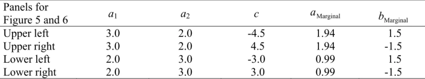
Table 4. Four 2-PL MIRT models and corresponding marginal parameter estimates
Panels for
Figure 5 and 6 a1 a2 c aMarginal bMarginal
Upper left 3.0 2.0 -4.5 1.94 1.5
Upper right 3.0 2.0 4.5 1.94 -1.5
Lower left 2.0 3.0 -3.0 0.99 1.5
Lower right 2.0 3.0 3.0 0.99 -1.5
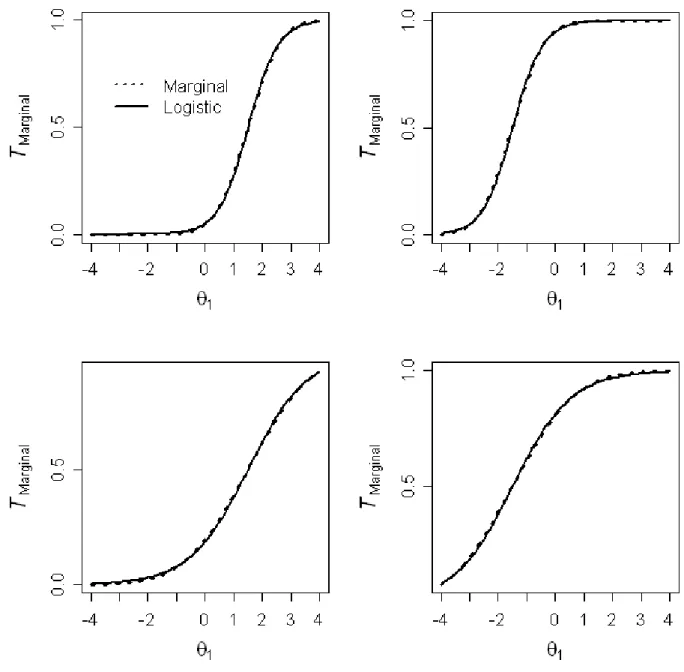
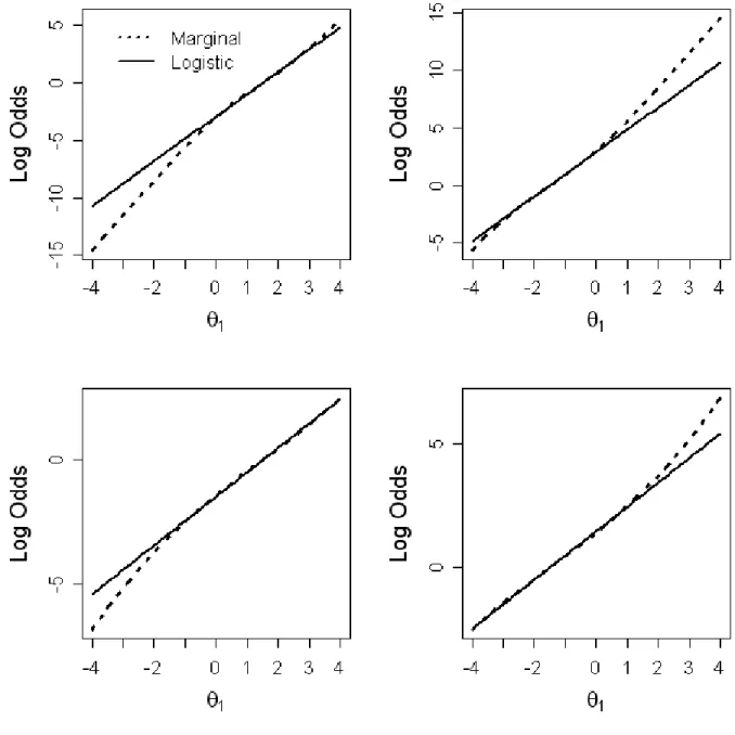
Figure 5 illustrates the close approximation between the logistic and marginal trace lines. The marginal is nearly indistinguishable from the logistic approximation, and appears to be unaffected by differences in location parameters, as suggested by Ip (2010a). Figure 6 illustrates the marginal trace lines and logistic approximations after a log odds
transformation. Because the logit of a logistic function is linear, the approximations will always be linear. The marginal however, can strictly speaking can never be linear, and any deviation represents missfit of the logistic approximation. The logits in Figure 6 illustrate this fact as deviations in marginals begin to appear in the tails of the distributions. However, at such extreme values in log odds, the probability equivalent is actually quite small (between 0.00002 and 0.003 at the most extreme values of θ1 for each comparison in Figure 6),
providing further evidence of the utility of the logistic as an appropriate appoximation.
Figure 5. Four 2-PL marginal trace lines and logistic approximations
Figure 6. Four 2-PL marginal trace lines and logistic approximations in log odds
The Relation Between Conditional and Marginal Slope Parameters
While Table 4 provides the marginal slope parameter of the logistic approximation for four sets of conditional slope parameters, in practice the computations needed to compute marginal slopes (equation 6) can be carried out for any combination of conditional slopes. Thus, it may be of some interest to provide the relation between conditional slope parameters and the resulting marginal slope parameter. Initially, the magnitude of the marginal slope for some simple bifactor MIRT models which have equal a1and a2slope parameters is
considered.
Figure 7. Marginal slopes for items with equal conditional slopes on two dimensions
Figure 7 illustrates the relationship between the magnitude of the marginal slope parameter and magnitude of the equal slopes on the primary and secondary dimensions. For
illustrative purposes, horizontal grey lines indicate increases in the marginal slope of 0.2 units, and correspond to marginal slopes of 1.1, 1.3, and 1.5. In general, when conditional slopes are weak (e.g., when aConditional is almost 1.5), the marginal slope is also weak and
only slightly less than the conditional slopes (e.g., aMarginal =1.1). The marginal slope
increases quickly from 1.1 to 1.3 with only slight gains in the conditional slopes. For example, increasing the conditional slopes about 0.5 units from 1.5 to 2.0 results in a marginal slope increasing about 0.2 units from a marginal slope of 1.1 to marginal slope of 1.3. However, gains in the marginal slope quickly diminish as the conditional slopes become large. Continuing with the present example, to achieve an additional gain in the marginal slope of 0.2 (i.e., aMarginal = 1.5) requires an increase in conditional slopes of more than 1.0
units (i.e., aConditional = 3.2). For most applications, conditional slopes constrained to be equal
will not be greater than this, because such slopes correspond to the dimensions accounting for nearly 90% of the item variance.
While conditional slopes much greater than this are unlikely and may be evidence of Heywood cases, they do illustrate an interesting fact of the marginal. For bifactor MIRT models with the conditional slopes constrained to be equal on two dimensions, the marginal slope is bounded by the logistic scaling constant. That is, as the conditional slopes increase, the item variance accounted for becomes nearly 50% for each dimension. Using (9) and (10), if the item variance explained is 50%, then the resulting marginal corresponds to the scaling constant (here, 1.7), or a factor loading of about 0.707.
For more general bifactor MIRT models with unequal conditional slopes, Appendix I may serve as a quick reference. The table provides the slope of the logistic approximation of the marginal trace line resulting from conditional slopes which vary from 1.00 to 4.50 in
29
increaments of 0.25. Because no current software programs compute marginal trace lines, the table should provide interested researchers with the magnitude of the marginal slope parameter for a wide variety of conditional slopes, and interpolation may be used for interpretation purposes.
Figure 8. Marginal slopes across a range of conditional slopes on two dimensions
1.0 1.5 2.0 2.5 3.0 3.5 4.0 4.5
01
23
4
1.0 1.5 2.0 2.5 3.0 3.5 4.0 4.5
a
1a
2Mar
gi
n
al
a1
CHAPTER 3
COMPUTING ITEM RESPONSE THEORY SCORES FROM MARGINAL TRACE LINES
This chapter considers the utility of using logistic approximations of marginal trace lines in a variety of test scoring applications. Specifically, logistic approximations of
marginal trace lines are used to compute unidimensional IRT-scaled scores for the general, or primary, dimension in bifactor IRT models. It is proposed that these scaled score estimates will provide a close approximation to the primary dimension point estimates used in
traditional MIRT scoring (Segall, 1996, 2000). In one recent example of MIRT scoring, Cai (2010) provides a two-tier algorithm in which the dimensionality of the integration for a multidimensional bifactor model is reduced to the number of primary dimensions plus one. Use of this estimation procedure results in a vector of ability estimates for the number of dimensions. From this vector of ability estimates, computed from the multivariate posterior density, the first element should be the same as the score estimate computed using the marginal posterior distribution (Segall, 2001).
1
ˆ
θ
The remainder of this chapter considers the degree to which unidimensional scoring computations using logistic approximations of marginal trace lines provide primary
dimension scores and standard error estimates similar to those obtained using the two-tier algorithm for multidimensional models. If the two methods are comparable, then use of the unidimensional logistic approximation technique may provide a simpler, less
comparison of IRT-scores and standard error estimates obtained from the logistic approximation of the marginal trace line with the conventional MIRT scoring technique implemented using the two-tier algorithm.
An Overview of IRT-Scaled Scores for Response Patterns and Summed Scores
Many applications of IRT-based scoring use the individual’s complete response pattern in forming the scaled score estimate. Known as response pattern scoring, the point-estimate is the mean or Expected A Posteriori (EAP) from the posterior distribution (Bock & Mislevy, 1982):
∏
, 12= =items i i i u T L 1 ) ( ) | ( ) |
(u θ θ φ θ
where the posterior distribution is the product of the trace lines for each response u to item i
and the prior density (here normally distributed with a mean of zero and a standard deviation of one). The mean of the posterior density may be computed by approximating the integral over a range of quadrature points q:
∑∏
∑∏
= =
≈ q items
i q q i iq q items i q q q i iq d u T d u T 1 1 1 1 ) ( ) ( ) ( ) ( ) ( EAP θ θ φ θ θ θ φ
θ . 13
Likewise, the standard deviation of any given posterior may also be computed by approximation:
∑∏
∑∏
= = −≈ q items
i q q i i q items i q q q i i d u T d u T D 1 1 1 1 2 ) ( ) ( ]) [ EAP )( ( ) ( ) ( S θ θ φ θ θ θ θ φ
θ . 14
As a function of the item parameters, the posterior standard deviation is allowed to fluctuate across the range of the latent variable.
While response pattern EAPs and SDs incorporate all available information from an individual’s responses to a set of items, the number of response patterns (i.e., the number of response categories to the power of the number of items) often makes tables of such response patterns, scores, and standard deviations unwieldy. As an alternative, one may compute the IRT-based expected value of the latent variable given the respondent’s summed score rather than response pattern. Scoring tables of summed scores and their associated EAPs and SDs are user-friendly alternatives to response pattern scores and are readily interpretable. It is possible to compute the expected value of the posterior for every summed score x which is itself the sum of the response vector u:
responsepatterns
( ) ( ) ( )
i
x
i x
L θ Tu θ ϕ θ
=
= ∑
∑ ∏
u
. 15
A recursive algorithm introduced by Lord and Wingersky (1984), and described in detail by Thissen, Pommerich, Billeaud, and Williams (1995), is used to computeLx(θ). Briefly, the recursive algorithm may be viewed as an updating process which is initialized by the trace line for a single item T1 where the likelihood for a summed score of 1 is Lx=1 = T1, and the
likelihood for summed score of 0 is Lx = 0 = (1-T1). When a second item is added to the test,
the likelihood of a summed score of 0 is (1- T1)*(1- T2); the likelihood for summed score of 2
is T1*T2; and the likelihood of summed score of 1 is the sum of T1(1-T2) and T2(1-T1). This
updating process continues until the likelihoods for all possible summed scores are evaluated. Because summed score based EAPs incorporate information available from all response patterns that yield a given summed score, and some of these response patterns may form likelihoods around different locations of the latent variable, any particular summed score likelihood will be slightly wider than the component response pattern likelihoods. For all but
the most extreme response patterns, the loss of information when using IRT-scores from summed scores results in score standard deviations being inflated about 10% (i.e., a 10% loss in precision (Thissen, et al., 1995)), though the correlation between response pattern and summed score-based EAPs is often greater than 0.95.
The decision to use IRT-scores from summed scores also allows intuitive and simple comparison between the two scoring methods. An advantage of using IRT-scores from summed scores is that they are a function of the previously estimated item parameters and all possible response patterns. Because these patterns are known and used in the recursive algorithm, there is no reliance on samples of individuals to provide IRT-scaled score estimates from summed scores.
Rather than comparing individual’s scaled scores using samples of response patterns, comparing summed score-based EAPs and SDs from the logistic approximation of the marginal trace line and the MIRT two-tier algorithm is quick and easy and may be computed directly from the MIRT item parameters. For instance, consider a multidimensional six-item binary test with seven possible summed scores on the primary dimension (0, ... , 6). Any difference in the seven EAPs between the two methods is interpreted as score bias when using the logistic approximations. The ratio between the score standard deviations represents potential bias in score precision between the two methods. For instance, if a particular score had standard deviation of 0.60 for the logistic approximation method and 0.80 for the two-tier approach, the ratio between the two-two-tier score standard deviations and logistic
approximation of the marginal trace lines (0.80/0.60) would indicate that the logistic
approximation scores appeared to be 1.33 times more precise. Such a finding would indicate
a bias of the logistic approximation method. Using such simple comparisons, many scores and standard errors can be evaluated from a variety of models.
The Method of Evaluating Primary Dimension Scores across MIRT Models
The methods used in this dissertation involve comparing scaled scores and score standard deviations between the logistic approximation and the two-tier algorithm for a variety of MIRT models (or tests) for binary items. All MIRT model parameter estimates are considered known.5 The steps involved for the comparisons are as follows: (1) For all
multidimensional tests, the primary dimension scaled scores from summed scores are initially computed using the two-tier algorithm, (2) next the marginal trace lines and logistic
approximations of them are computed for all items using the methods presented in Chapter 2, (3) finally, the recursive algorithm is used to compute the comparable primary dimension scores and score standard deviations from the logistic approximations. These steps are repeated for all tests.
To evaluate the utility of scoring tests using the logistic approximation of the marginal trace line, the two scoring approaches are compared across a variety of MIRT models. Comparisons between the two methods will take into account three model-related conditions,
factor loadings, test length, and dimensionality. The following model conditions are meant to reflect a wide range of bifactor models used in research settings.
First, to compare models which vary in influence of the secondary dimension, the factor loading6 conditions will consider different ratios between the magnitude of the primary and secondary dimension loadings. A range of factor loadings will be divided into three groups
5 For simplicity, the thresholds of all MIRT parameter estimates (modeled as intercepts) were fixed at
the mean of the latent variable (θ = 0). Findings in Chapter 2 indicate that fit of the logistic
approximation to the marginal trace line is independent of the location of item’s location parameter.
6
To provide a more readily interpretable metric, factor loadings are reported. All computations were
performed with slope parameters converted from factor loadings.
(low (.3 to .5), medium (.5 to .7), or high (.7 to .9)), following guidelines used by McDonald
(1999) and Reise, Cook, and Moore (under review). Items with multidimensional structure may
have primary and secondary dimension slopes which are combinations of low, medium, and high (e.g., “high” primary and “low” secondary, “low” primary and “high” secondary”, etc.). Note that “high” factor loadings on both the primary and secondary dimensions may result in negative residual variances or so-called Heywood cases. Thus, this condition was eliminated resulting in eight different primary and secondary factor loading conditions. Varying the factor loadings across dimensions in this manner provides a means of detecting potential biases in scores based on the strength of a particular dimension. These biases, however minor, may be compounded depending on the strength of loadings and test length.
In addition to differences in factor loadings across dimensions, it is also of interest to consider multiple test lengths. For instance, for a long test with one pair of LD items, there may be little utility in computing the marginal trace line given simpler traditional methods (e.g., setting items aside to eliminate LD), whereas for a short test, which provides less score information, it may be more desirable to consider marginal trace lines as a means of gaining all possible information from the data. Thus, to uncover how the test length condition affects scoring the logistic approximations, a few practical test lengths are considered. Based on common lengths of scales in both health outcomes and psychological research, short (6 items), medium (12 items), and long (24 items) tests are considered.
Finally, the design of the dimensionality condition will take into account two model fitting situations in which bifactor models are commonly used. The first situation is one in which all items load on both the primary dimension and, because of hypothesized
dependence among clusters of items, one secondary dimension (i.e., complete bifactor
structure). The second situation represents a modified-bifactor model in which the items are generally unidimensional, but because of some unplanned nuisance dimensionality,
secondary factors in the form of item doublets are needed to achieve conditional
independence. For both situations, the number of item clusters and doublets modeled is dependent on the length of the test. For instance, while a short test may be limited to one or two secondary dimensions (modeled as doublets, or two locally dependent items), the medium and long test length conditions includes high-dimensional models which have only recently become practical following advances in MIRT parameter estimation via the two-tier method (Cai, 2010). Because the number of dimensions possible depends on test length, or is nested within test length, the dimensionalitycondition allows the short test condition to have 1 or 2 secondary dimensions (i.e., 1 or 2 doublet pairs); the medium length test has 3
secondary dimensions with 4-item clusters or 3 doublet pairs of items; and the long test has 6 secondary dimensions with 4-item clusters or 6 doublet pairs of items.
Given these conditions, the study design crosses the strength of the factor loadings on the primary and secondary dimensions with test length (and also the number of dimensions that are nested within test length). This scoring design results in three factor loading
conditions (which when crossed yields 8 conditions), three test length conditions, and two dimensionality conditions within each test length condition. The total number of conditions which compare scores computed from the logistic approximation to the two-tier algorithm is then 8factor loadings x 3test length x 2dimensionality = 48. This study design covers the majority of test
conditions seen in research settings. These conditions provide insights into the use of logistic approximations of marginal trace lines in providing a better understanding of the relation
between item responses and the primary dimension, and if so, whether or not these techniques are useful in providing an IRT-score for the primary dimension.
An IRT-based Scoring Example
To further illustrate these MIRT scoring conditions, this section follows one of the forty-eight conditions through the entire scoring process. This condition uses the long test (24 items), with complete bifactor structure (six secondary clusters with four items each), and has medium factor loadings on the primary dimension and low factor loadings on the secondary dimensions. The multidimensional factor structure is provided in Table 5. Note from the table that the primary dimension loadings are balanced between the lower (.5) and higher (.7) loadings for the “medium” factor loading condition, and the secondary dimension loadings are balanced between the lower (.3) and higher (.5) loadings for the “low” factor loading condition.
Table 5. Example of bifactor structure for scoring.
Item λ1 λ2 λ3 λ4 λ5 λ6 λ7
1 0.5 0.3
2 0.6 0.3
3 0.6 0.3
4 0.7 0.3
5 0.5 0.4
6 0.6 0.4
7 0.6 0.4
8 0.7 0.4
9 0.5 0.5
10 0.6 0.5
11 0.6 0.5
12 0.7 0.5
13 0.5 0.3
14 0.6 0.3
15 0.6 0.3
16 0.7 0.3
17 0.5 0.4
18 0.6 0.4
19 0.6 0.4
20 0.7 0.4
21 0.5 0.5
22 0.6 0.5
23 0.6 0.5
24 0.7 0.5
After converting the factor loadings in Table 5 into slopes, the two-tier algorithm, as implemented in the software program IRTPRO (Cai, du Toit, & Thissen, forthcoming) is used to compute primary dimension IRT-scores and standard deviations along with their associated summed scores. After tabulating these values, the marginal trace lines for all 24 items are computed from the MIRT item parameters using the R language for statistical computing and 81 quadrature points equally spaced between -4 and +4. Logistic
approximations using the 2PL model are then made from these marginal trace lines. Once the 2PL item parameters are obtained, the recursive algorithm is used to compute the IRT-scaled scores and standard deviations from summed scores. This process results in two sets
of IRT-scaled scores and score standard deviations for the primary dimension. A summed score to scale score translation table is then used to compare the values from the two approaches. Below, Table 6 provides the results for this first of forty-eight scoring comparisons.
Table 6. Example of a score translation table using the logistic approximation of marginal trace lines and the two-tier algorithm.
Summed Score Two-Tier EAP Logistic EAP Two-Tier SD Logistic SD
0 -2.07 -2.17 0.59 0.56
1 -1.73 -1.83 0.53 0.50
2 -1.47 -1.56 0.49 0.45
3 -1.25 -1.33 0.46 0.42
4 -1.07 -1.13 0.44 0.39
5 -0.90 -0.95 0.42 0.36
6 -0.75 -0.79 0.41 0.35
7 -0.61 -0.64 0.40 0.33
8 -0.48 -0.50 0.39 0.32
9 -0.36 -0.37 0.39 0.32
10 -0.24 -0.25 0.38 0.31
11 -0.12 -0.12 0.38 0.31
12 0.00 0.00 0.38 0.31
13 0.12 0.12 0.38 0.31
14 0.24 0.25 0.38 0.31
15 0.36 0.37 0.39 0.32
16 0.48 0.50 0.39 0.32
17 0.61 0.64 0.40 0.33
18 0.75 0.79 0.41 0.35
19 0.90 0.95 0.42 0.36
20 1.07 1.13 0.44 0.39
21 1.25 1.33 0.46 0.42
22 1.47 1.56 0.49 0.45
23 1.73 1.83 0.53 0.50
24 2.07 2.17 0.59 0.56
Note: Because the difficulty parameters are fixed at zero for all items, the EAP and standard deviations are symmetrical around the mean 0.0.
This table provides the first appearance of bias in scoring when using the logistic approximations of marginal trace lines. For each summed score, across the entire range of
the primary dimension, the scaled scores for the logistic approximation are more extreme than those computed directly from the MIRT model. Though potentially minor, the
difference in the logistic-based point estimates is at most ±0.10 standard deviations from the two-tier-based estimate. Additionally, the standard deviations indicate overly narrow posteriors for the logistic approximation (a spurious increase in score precision of about 5% to 18% depending on the location of the latent variable). In other words, the logistic
approximation gives the impression that the items provide more information about the latent variable than should be present.
Prior to scoring all 48 conditions, this phenomena, where use of the logistic
approximation of the marginal trace line results in a spurious increase in score precision (i.e., overly precise scores), is investigated in a few selected conditions. Figure 9 provides a graphical illustration of the values in Table 6. Parallel results for a 12-item scale with medium slopes on the primary dimensions and low secondary slopes with three doublet factors are shown in Figure 10, and results from an example with one doublet, 6-item scale with high slopes on the primary dimension and medium slopes on the secondary dimension are in Figure 11.
Figure 9.
0
5
10
15
20
25
-0.1
0.0
0.1
Summed Score
θ
^
Prim
a
ry
−θ
^
Logi
st
ic
Long scale, six clusters
(
λ
P=
0.5
−
0.7
, λ
S=
0.3
−
0.5
)
0
5
10
15
20
25
1.0
1.2
Summed Score
σ
Prim
a
ry
σ
Logi
st
ic
Figure10.
0 2 4 6 8 10 12
-0.05 0.00 0.05
Summed Score
θ
^
Prim
a
ry
−θ
^
Logi
st
ic
Medium scale, three doublets
(
λ
P=
0.5
−
0.7
, λ
S=
0.3
−
0.5
)
0 2 4 6 8 10 12
0.9 1.0 1.1 1.2
Summed Score
σ
Prim
a
ry
σ
Logi
st
ic
Figure 11.
0 1 2 3 4 5 6
-0.10 -0.05 0.00 0.05 0.10
Summed Score
θ
^
Prim
a
ry
−θ
^
Logi
st
ic
Short scale, one doublet
(
λ
P=
0.7
−
0.9
, λ
S=
0.5
−
0.7
)
0 1 2 3 4 5 6
0.9 1.0 1.1
Summed Score
σ
Prim
a
ry
σ
Logist
ic
The figures illustrate the difference between primary dimension EAPs and SDs between the two-tier algorithm and the logistic approximation of the marginal trace line. The upper panel of each figure indicates the differences in EAPs between the two scoring methods. Because the thresholds are fixed at zero, the mean IRT score is always 0.0 and is located in the middle of the summed score scale. For instance, in Figure 9 the mean summed score is 12 (out of 24) and is associated with an EAP of 0.0. EAPs for summed scores greater than 12 are positive values, and EAPs less than 12 are negative values. In all figures, when the difference between two-tier and logistic approximation EAPs is positive for summed scores below the mean, the difference indicates that the logistic approximation is providing an EAP which is lower than the EAP for the two-tier algorithm.
The lower panel of each figure indicates the ratio in score standard deviations of the two-tier algorithm to the logistic approximation. Because all ratios are greater than 1.0, each of the three examples indicates that use of the logistic approximation provides overly precise score estimates (i.e., overly narrow posteriors).
The pattern of results is also similar across the three examples. That is, the logistic approximations of marginal trace lines produce more extreme scores and scores with more apparent information. While there appear to be differences in the magnitude of these deviations, the patterns remain consistent. The logistic approximation provides overly precise scores near the mean of the latent variable, and performs somewhat more expectedly near the tails of the distribution. The EAPs for scaled scores at the mean are exactly the same as the two-tier algorithm suggests, indicating that the mean summed score is the middle value and corresponds with an EAP of zero. However, differences from the mean are
symmetrical such that the logistic approximation-based EAPs suggest scores that are farther
from the mean of the latent variable than the two-tier algorithm provides (i.e., more extreme scores).
Controlling Local Dependence
Differences between scaled scores and standard deviations in Figures 9-11 indicate the same problem: More weight or information is being provided by the logistic approximations of marginal trace lines. These findings may be best explained by a failure to account for local dependence. In other words, while the marginal slope does provide the relation between the item response and the primary dimension after controlling for the secondary dimension(s) for each given item, it does not take into account the other items loading on the same dimension. Each item’s marginal slope is the correct relation between the item
response and the primary dimension for the individual item, but pooling multiple items from the same secondary dimension is still in essence providing more items of the type that are described by the secondary dimension, which is a violation of local independence when scored with a unidimensional model.
This phenomenon may be explained through an example. Suppose responses to a set of items were best characterized by a bifactor model in which negative affect is the primary dimension, but with the secondary factors anger, anxiety, and depression. If a researcher using only the anger subdomain items was interested in a score for the general factor, negative affect, then (as was proposed) computing the marginal trace lines for the negative affect dimension (integrating over the anger secondary factor) should provide the parameters to be used in IRT-based scoring. However, this suggestion essentially ignores the items’ multidimensionality and treats them as if they were a unidimensional set measuring negative