Entropy-based Correspondence Improvement of
Interpolated Skeletal Models
Liyun Tua,b,1, Jared Vicoryb,1,∗, Shireen Elhabianc, Beatriz Paniaguab,
Juan Carlos Prietod, James N. Damonb, Ross Whitakerc,
Martin Stynerb, Stephen M. Pizerb
a
Chongqing University, Shapingba, China b
University of North Carolina at Chapel Hill, Chapel Hill, NC, USA c
University of Utah, Salt Lake City, UT, USA d
Brigham and Women’s Hospital, Boston, MA, USA
Abstract
Statistical analysis of shape representations relies on having good correspon-dence across a population. Improving corresponcorrespon-dence yields improved statistics. Point distribution models (PDMs) are often used to represent object boundaries. Skeletal representations (s-reps) model object widths and boundary directions as well as boundary positions, so they should yield better correspondence.
We present two methods: one for continuously interpolating a discretely-sampled skeletal model and one for improving correspondence by using this interpolation to shift skeletal samples to new positions. The interpolation op-erates by an extension of the mathematics of medial structures. As with Cates’ boundary-based method, we evaluate correspondence in terms of regularity and shape-feature population entropies.
Evaluation on both synthetic and real data shows that our method both improves correspondence of s-rep models fit to segmented lateral ventricles and that the combined boundary-and-skeletal PDMs implied by these optimized s-reps have better correspondence than optimized boundary PDMs.
Keywords: Statistical Shape Analysis, Correspondence, Skeletal Models
1. Introduction
Statistical analysis of shape populations is an important task in many image analysis applications. Achieving good correspondence [1] across a population of shapes is a necessary step in computing accurate statistics. For point distri-bution models (PDMs) [2], this means having the points evenly spread around the object while each point has similar local geometry on every object. The
∗Corresponding author. Phone:+1 919 886 5757 Email: [email protected]
most common use of the PDM is to represent the boundary of an object. Cates et al. [3] developed a method for improving correspondence of a set of PDMs by shifting points along the boundary to minimize geometric entropy less a regularity entropy summed over the population, which is implemented in the publicly availableShapeWorks [4] software. This optimization has been shown to produce improved statistics on populations of PDMs.
In many applications [5, 6, 7], it is beneficial to model object interiors as well as boundaries. Skeletal representations (s-reps) [8] are one method for do-ing this. An s-rep consists of a discretely sampled skeletal surface with vectors called spokes pointing from the skeleton to the object boundary. As with PDMs, good correspondence is required for statistical analysis of s-reps. At the same time, it would be interesting to compare the statistical properties of a boundary PDM put into correspondence directly by the Cates method to one implied by the s-reps correspondence. In this paper, we present a method for improving correspondence of s-reps by shifting spokes along the skeleton. Similarly to the boundary-based method, we shift spokes to minimize a geometric entropy less a regularity entropy summed over the population. In order to shift these discrete spokes, we develop a method for interpolating a continuous s-rep from the dis-crete samples. The interpolation is a new result generalizing the mathematics of medial structures [9].
We evaluate our method on a set of 31 lateral cerebral ventricles. We show that our method improves the correspondence of s-reps fit to this data. We also compare the results of the s-rep correspondence optimization to two methods of producing corresponding PDMs: the PDMs computed via the SPHARM-PDM [10] method as well as SPHARM-PDMs optimized using the ShapeWorks software. To compare s-reps to the PDM data, we apply our measures of correspondence to the PDM implied by the s-rep spoke ends.
The rest of this paper lays out as follows. Sections 2 and 3 provide back-ground information and a brief description of materials. Section 4 describes our method for interpolating continuous object interiors from discrete s-reps. Sec-tion 5 describes our method for improving the correspondence of s-rep models using an entropy-minimizing optimization. Section 6 gives results of applying the s-rep correspondence optimization, and section 7 discusses these results, gives conclusions, and describes future work.
2. Background
2.1. Entropy-based surface correspondence
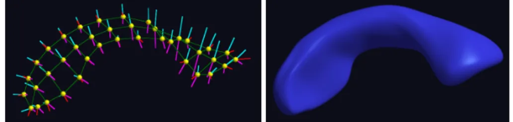
Figure 1: An s-rep model (left) and its implied boundary (right). The yellow balls are samples of the skeletal surface. The cyan spokes point to the top of the object, the magenta to the bottom, and the red to the crest. The green lines show the grid structure of the skeletal samples.
to improve correspondence across a population of objects [3]. This method takes an existing set of PDMs and shifts the points along the interpolated boundary to optimize an objective function which is a difference of two terms: ageometry entropywhich measures how well some set of geometric features at a point match across the population, and aregularity entropy which measures how evenly the points are spread within each case. The idea is that the geometric probabil-ity distribution should be tightened while the probabilprobabil-ity of boundary point positions should be made more uniform on each case.
2.2. Skeletal Models
The s-rep [8] is a quasi-medial skeletal model that models not only an object’s boundary but its interior as well. The s-rep is a collection of points sampled from a skeleton of an object which have associated vectors calledspokespointing from the skeleton to the object’s boundary. This model is fit to an object via an optimization which requires the skeleton to be as close to medial as possible while remaining non-branching and requires the spokes to touch the object boundary and be nearly orthogonal to it [8]. As such, it captures not only object positions but also object widths and object boundary directions. These samples can then be interpolated to produce a continuous representation of an object’s boundary and interior. This provides an object-relative coordinate system (u, v, τ) for the object’s volume, where (u, v) parameterizes the skeleton andτ moves from the skeleton (τ= 0) to the boundary (τ = 1).
2.3. Composite Principal Nested Spheres
Because shapes in general, and s-reps in particular, have many features which do not naturally live in a flat Euclidean space, standard Euclidean statistical techniques such as principal component analysis (PCA) have proven inadequate for analyzing populations of s-reps. Instead, because many s-rep features live on spheres, such as the spoke directions (S2) and the PDM formed from then
skeletal points (S3n) [11], a method that can analyze data directly on spheres
is preferred.
best-fitting subspaces of codimension 1 onto which the data is projected, PNS successively computes best-fitting subspheres, lowers the dimension by projec-tion, and repeats. At each projection step, the signed geodesic residual of each data point to the subspace is recorded. It is reasonable to treat this collection of signed distances as a Euclidean data object and analyze it using standard meth-ods. We call this process Euclideanization. By combining these Euclideanized features with the originally-Euclidean features and being careful to scale the Euclideanized features to make them commensurate, all of the data can now be analyzed using standard PCA. This method is called composite principal nested spheres (CPNS) [13].
3. Materials
The objects on which the methods described herein are evaluated consist of 31 lateral cerebral ventricles of neonates segmented from MRI. The subjects were at risk for schizophrenia or bipolar disorder.
Each ventricle was fit via the SPHARM-PDM [14] toolbox and 1002-point PDMs were extracted at corresponding latitudes and longitudes. An s-rep was fit [8] to the solid implied by each SPHARM.
4. Spoke Interpolation
4.1. Skeletal Mathematics
A continuous skeletal model describes an object interior by two functions: p(u1, u2), a 2D skeletal surface and S(u1, u2), a vector field pointing from the
skeletal surface to the boundary. Scan be further decomposed into a product of two functions: U(u1, u2), a unit vector field pointing in the direction of S
and r(u1, u2), a scalar distance function from the skeletal sheet to the object
boundary.
An s-rep is a sampling of the continuous skeletal model. It consists of an
m×ngrid of samples from the skeletal surface with either two spokes (on the
interior) or three (along the crest). The grid structure on the skeletal sheet forms a collection of quadrilaterals with a skeletal sample at each corner.
From this discrete representation we require a method to interpolate back to the continuous entity. Our method is a generalization to quasi-medial objects of the method for interpolating medial representations (m-reps) [15], which was based on the mathematics of medial structures [9].
We wish to interpolate a spokeS(u∗
1, u∗2). If the sampled skeletal points have
integer parameter values, (u∗
1, u∗2) can be written as
(u∗
1, u∗2) = (u01+δu1, u20+δu2); δu1, δu2∈[0,1)
where (u0
1, u02) is the top left corner of the quad containing the desired value.
S(u∗
1, u∗2) =S(u01, u02) +
(δu1,δu2) I (0,0) ∂ S ∂u1
du1+
∂S
∂u2
du2
(1)
for the spoke we wish to interpolate. SinceS(u1, u2) =r(u1, u2)U(u1, u2), the
partial derivatives in equation 1 can be written asSui =rUui+ruiU.
The radius derivatives rui can be computed using the equation [16, 17] −rui =pui·U+Bui·U, whereBui are boundary derivatives, (B=p+rU=
p+S and Bui = pui +Sui). This equation is a correction to the
compati-bility condition for medial models [9] necessary because boundary and skeletal changes are not tied together as strongly in skeletal models as in medial ones. Using this expression forrui, we obtain
Sui =rUui−(pui·U+ (pui+Sui)·U)U=rUui−(2pui+Sui)U TU
= rUui−2puiU TU
I+UTU−1 (2)
This equation allows for the computation of the spoke derivative at any point (u∗
1, u∗2) given the derivative of the skeletal surfacepui and spoke directionUui
at that point. Section 4.2 describes a method for computingpui, while 4.3 deals
with computation ofUui. Finally, 4.4 describes how a spoke is interpolated via
numerical integration of equation 2.
4.2. Interpolation of the Skeletal Surface
Interpolation of the skeletal surface is done by fitting cubic Hermite patches to the quads of discrete samples which form the surface. This interpolation re-quires 16 values: the (4) corner pointsp(u0
1, u02),p(u11, u02),p(u01, u12),p(u11, u12),
the (8) derivatives of each corner in both parameter directions, and the (4) sec-ond order mixed partial derivatives, which are set to 0. The control matrixHc
is thus
Hc=
p(u0
1, u02) p(u11, u02) pu2(u 0
1, u02) pu2(u 1 1, u02)
p(u01, u12) p(u11, u12) pu2(u 0
1, u12) pu2(u 1 1, u12)
pu1(u 0
1, u02) pu1(u 1
1, u02) 0 0
pu1(u 0
1, u12) pu1(u 0
1, u02) 0 0
LetH(s) = (H1(s), H2(s), H3(s), H4(s)) andH′(s) = (H1′(s), H2′(s), H3′(s), H4′(s))
whereHi are the cubic Hermite spline basis functions andHi′ are their
deriva-tives. Computation at a point (u∗
1, u∗2) inside a quad is given by
p(u∗
1, u∗2) =H(δu1)·Hc·H(δu2)T.
Derivatives of the skeletal surface are computed by replacing the appropriate set of basis functions by their derivatives:
pu1(u ∗
1, u∗2) =H′(δu1)·Hc·H(δu2)T; pu2(u ∗
1, u∗2) =H(δu1)·Hc·H′(δu2)T
4.3. Estimation of Spoke Direction Derivatives via Quaternion Interpolation In equation 2, the derivatives of the spoke direction vector field Uui are
needed. BecauseU is a unit vector field, changes in U are purely rotational. Thus, we choose a quaternion-based interpolation to compute these derivatives. Each spoke direction at the corner of a quad is represented by a quater-nion. A unit vector U = (Ux, Uy, Uz) is represented by the quaternion q =
0 +Uxi+Uyj+Uzk. From the four spoke quaternions bounding a quad we can
interpolate a unit quaternion in the quad interior by spherical linear interpola-tion (slerp) [18]. The quaternion that isλ(∈[0,1]) of the distance betweenqi
andqi+1 is given bySL(qi,qi+1, λ) =qi(q∗iqi+1) λ
.
To achieve higher continuity across quad boundaries and thus a smoother surface, a higher order interpolation is desired. We use an extension of the cubic B´ezier curve to the surface of a sphere called squad [19]. Analogously to the application of De Casteljau’s algorithm to the computation of B´ezier curves, squad can be computed in terms of slerp:
SQ(qi,qi+1,ai,ai+1, λ) =SL(SL(qi,qi+1, λ), SL(ai,ai+1, λ),2λ(1−λ)) (4)
whereaiandai+1are B´ezier curve control points. Careful choice of these points
ensuresC1 continuity across theq
is [19][20]:
ai=qiexp
−log(q
−1
i qi+1) + log(q−i1qi−1)
4
Differentiating the spoke interpolation formulaSQwith respect toλyields [20]
SQ′(q
i,qi+1,ai,ai+1, λ) =SL(qi,qi+1, λ) log(q∗iqi+1)gi(λ)2λ(1−λ)+
SL(qi,qi+1, λ)
g′
i(λ)2λ(1−λ)
(5)
wheregi(λ) =SL(qi,qi+1, λ)∗SL(si,si+1, λ).
The derivativeUu1(u∗1, u∗2) within a quad is computed by first using equation
4 to estimate U(u−1
1 , uδu2 2),U(u01, uδu2 2),U(u11, uδu2 2), and U(u21, uδu2 2) via the
4×4 surrounding grid spokes. Equation 5 on the resulting quaternions then
yields the desired derivative. The computation is similar forUu2.
4.4. Spoke Computation via Integration of Derivatives
With the pui and Uui values from sections 4.2 and 4.3, we can start from
the quad corner (u0
1, u02) and integrate equation 2 using interval subdivision h
to produce a spoke at (uh
1 =u01+hδu1, uh2 =u02+hδu2). Euler’s method for the
integration yieldsS(uh
1, uh2) =S(u01, u02) +h δu1Su1(u 0
1, u02) +δu2Su2(u 0 1, u02)
. From (uh
1, uh2), we take another step towards (u∗1, u∗2) and iterate to (u∗1, u∗2).
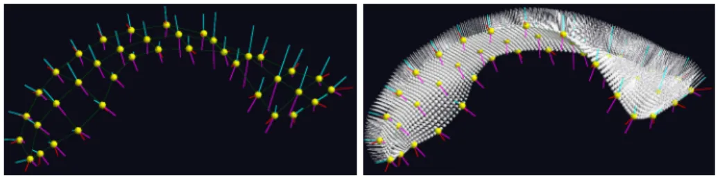
Figure 2: A lateral ventricle s-rep and a dense interpolation of its top side spokes.
5. Correspondence
In this section we describe our method for improving s-rep correspondence through spoke shifting. Tightening the probability distribution of the geometric properties of s-reps in the population is the basic means of producing correspon-dence. If this is optimized alone, these features will tend to group together and produce highly irregular objects. This effect is avoided by also considering, for each training object, an entropy derived from various s-rep properties related to the regularity of the distribution of spokes throughout the s-rep. We improve s-rep correspondence by optimizing the weighted difference of these two entropy measures.
5.1. Spoke Shifting to Optimize Entropy
In order to optimize correspondence, spokes must be able to shift along the skeletal surface while respecting the boundary of the object. A spoke
S(ui, vj), with i, j ∈ Z+, is shifted to a new position S(ui +δui, vj +δvj)
by interpolating the value of the spoke atS(ui+δui, vj+δvj). By constraining
δu, δv∈(−0.5,0.5), we ensure that the rectangular structure of the grid is kept
intact. Spokes in the interior of the grid shift along the skeletal surface, while spokes along the fold of the object can only move on the crest curve.
The δu and δv by which the spokes are shifted are chosen to optimize an objective function which is the difference of two entropies: a geometry term
Egeowhich measures how well corresponding spokes match across a population
of objects and a regularity term Ereg which measures how evenly spokes are
distributed within each object. The following subsections discusses each of these terms in more detail.
5.2. Geometry Entropy
estimated via standard Euclidean PCA, from which the entropyEgeo is
com-puted.
5.3. Regularity Entropy
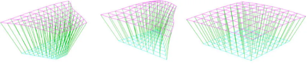
The regularity entropy is a measure of how uniformly distributed features are within each object. On an s-rep, using spoke interpolation the grid of skeletal positions can be connected to form curvilinear quadrilaterals with corresponding curvilinear quads on the object boundary. Figure 3 shows three examples of these quads with varying regularity.
Figure 3: Three s-reps with varying regularity. The quads of the left and middle s-reps are non-regular while the right s-rep is highly regular.
S-rep regularity is measured on a number of features for each skeleton / boundary quad pair. We wish these features to be statistically independent while implying the geometrical properties of quad edge lengths, quad areas, and inter-quad-pair volumes, which are intuitively related to regularity. The features are as follows: horizontal and vertical quad edge lengths, average angle cosines of top-left and bottom-right corners of each interpolated sub-quad, and cosine of the swing of the quad normal between the two corners of the quad. The first two help to enforce regular shapes for the quads (tend towards rectangles) while the last penalizes highly curved surfaces (tends toward planar quads). These properties are computed separately for the skeleton and boundary quads. The similar features for each quad are combined (i.e., the boundary and skeletal horizontal edge lengths for that quad are concatenated) forming a tuple of that feature for that quad. These features are then combined from all quads into three groups: the horizontal edge lengthsMhel, the vertical edge lengthsMvel,
and the angle cosinesMcos. If there are 2kcopies of a feature per quad (kon
the boundary andk on the skeleton) and there are n quads in the s-rep, this yields a 2k×nfeature vector.
From these three feature sets, the entropy measures Ehel, Evel, and Ecos
are derived (see section 5.4 for detail on the Entropy computation). The total measure of regularity forithobject in the training set isEi
reg =Eheli +Eveli +Eicos
due to the assumption of independence.
5.4. Optimization
Gaussian distribution. The entropy of a d-dimensional Gaussian random vari-able X is H(X) = 12d+dln(2π) +Pd
i=1lnλi
, where λ1, λ2, . . . λd are the
non-zero eigenvalues of the covariance matrix ofX. Because in many applica-tions the covariance matrix will not have full rank, there will be a number of small eigenvalues that will disproportionately contribute to H(X). We solve this by removing eigenvalues with contributionλi/Pλi lower than a threshold
θ.
We optimize correspondence by minimizing
arg min
x
ωEgeo(x)−
N
X
i=1
Ei reg(x)
!
(6)
where ω is a weight controlling the balance between probability distribution tightness and the regularity of each model and xis the shifting of each spoke in all of the models. The optimization is done via iterative, alternating appli-cations of the NEWUOA [21] and one-plus-one evolutionary [22] optimization algorithms. The choice of the parameters ω and θ was made via empirical evaluation.
6. Application & Results
Our method was first tested on a set of 80 synthetic lateral ventricle s-reps where all but one spoke were identical. After optimization, the distribution of the one moving spoke was greatly tightened.
In the following experiments we evaluate the method for improving s-rep correspondence on the set of 31 lateral ventricle shapes described in section 3. Unless otherwise noted, for these experimentsω= 4 in equation 6 andθ= 0.01.
6.1. Improvement of S-rep Correspondence
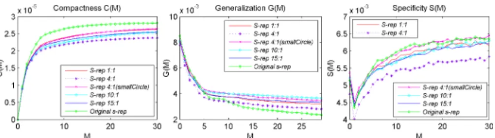
Figure 4 shows distributions of s-rep spokes before and after optimization. The s-reps after optimization have qualitatively better correspondence and main-tain good regularity properties.
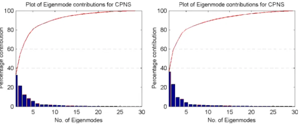
Figure 5 shows the cumulative variance explained by each eigenvalue from CPNS analysis on the s-rep population, i.e. of the s-rep features, before and after optimization. The two plots are similar, but after optimization the amount of variance captured in the first two eigenmodes has increased. The cumulative variance of the s-rep population is lower after optimization, with the sum of the eigenvalues being .0081 compared with .0085 before optimization.
Figure 4: Distributions of spokes on the top (left) and crest side (right) of the s-reps before (first row) and after (second row) optimization. The groupings of spokes are noticeably tighter after optimization.
Compactness is a measure of tightness of a probability distribution, com-puted as the sum of the eigenvalues obtained via PCA. After correspondence optimization there is marked improvement in compactness.
Generalization is measured by computing a shape space on all but one of the training cases and computing the distance between the last shape and its projection onto this shape space. Generalization is computed on a set of PDMs in a leave-one-out fashion. PCA is applied to all but one case, forming a shape space. This final PDM is then projected onto the shape space given by the firstM modes of variation. The distance between the PDM and its projection is computed as the average Euclidean distance between pairs of correspond-ing points. The optimized s-reps show slightly better generalization for low
Figure 6: Plots of compactness (left), generalization (center), and specificity (right) on the original and optimized s-rep populations. These measures are functions of the number of eigenmodes (M) used to form the shape space.
Figure 7: Effects of the weighting factorωon the 31 lateral ventricle s-reps on compactness
(left), generalization (middle), and specificity (right).
numbers of eigenvalues that would be used in a final model as indicated by the compactness result. However, they show slightly worse generalization than before optimization at higher numbers of eigenvalues.
Specificity is a measure of average distance between random samples in the computed shape space with their nearest members of the data. Specificity is computed by using PCA on all PDMs to produce a probability distribution. Independent random samples are chosen from the distribution given by the first
M modes. For each sample, the distance between it and the nearest original PDM is computed in the same way as for generalization. The optimized s-reps show noticeable improvement in specificity.
We did not evaluate the accuracy of boundary positions interpolated from the modified s-reps as in application we interpolate these from the original s-rep rather than the modified one.
We also examined the effect of changing the weightω on the results of the optimization. Figure 7 shows the correspondence measures on s-reps with differ-ent weights. In general,ω= 4 is the best choice, showing the most improvement in compactness and specificity and the least worsening of generalization.
6.2. Comparison with PDM-based Methods
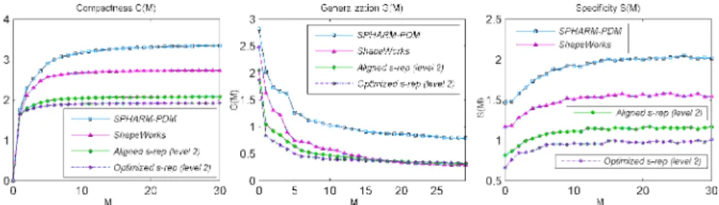
Figure 8: Plots of compactness (left), generalization (middle), and specificity (right) measures of the original SPHARM-PDMs, the s-reps after correspondence optimization, and the PDMs optimized via ShapeWorks. These measures are functions of the number of eigenmodes (M) used to form the shape space.
For SPHARM-PDM and ShapeWorks, these measures are directly on the bound-ary PDMs. For the s-reps, use the PDMs mentioned previously. All PDMs have similar numbers of points, with the s-reps being interpolated to match the num-bers of points in the SPHARM-PDMs. Figure 8 shows comparisons of the three methods using the three correspondence evaluation criteria. The s-rep-implied PDMs are scaled to match the scale of the others.
For compactness, the optimized s-reps show noticeably improved compact-ness over both of the PDM datasets. For generalization, the optimized s-reps are better than both for low numbers of eigenvalues but worse than the op-timized PDMs at higher numbers. For specificity, the opop-timized s-reps again out-perform both PDM datasets.
7. Discussion
This paper presented novel methods for interpolating discrete s-reps into continuous objects and improving the correspondence of a population of s-reps. This interpolation is an extension of the interpolation of m-reps to the more general skeletal representation. The correspondence improvement is done via entropy minimization analogously to similar methods for PDMs. This opti-mization was shown to improve the correspondence of a population of lateral cerebral ventricle s-reps and s-rep-implied PDMs are shown to have correspon-dence comparable to or better than PDMs optimized via ShapeWorks.
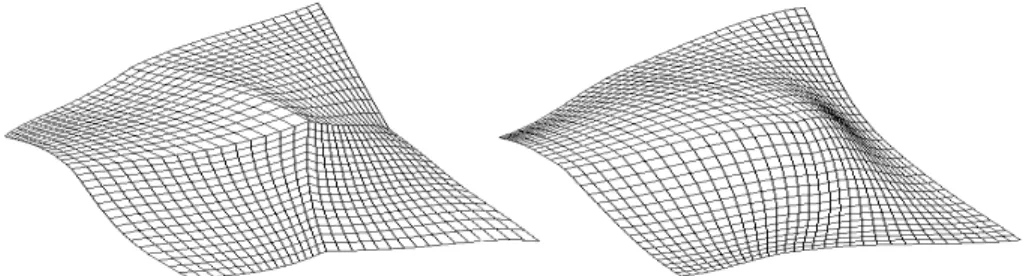
The interpolation method presented here produces smoother and more accu-rate s-rep boundaries, as earlier methods for s-rep interpolation were based on the mathematics of medial structures and failed to correctly model the interac-tion between changes in the skeleton and the boundary when medial constraints are relaxed. Figure 9 shows a comparison of a boundary patch interpolated using both methods. The use of Euler’s method for performing the integration steps will be replaced by a method with better speed and accuracy properties in future work.
Figure 9: Comparison between interpolations of an s-rep using medially-based (left) and skeletal-based (right) mathematics.
without improved correspondence outperform PDMs in the statistical tasks of classification [7] and hypothesis testing [26] and we believe that using s-reps with improved correspondence will only further this advantage. In particular, the results on compactness show that the improved s-reps are a more efficient representation than the non-optimized s-reps used in previous studies, while the similar generalization and improved specificity suggest the improved s-reps could be more powerful for these tasks. Experiments to demonstrate this im-provement are planned but are outside the scope of this paper.
The comparisons done to the PDM datasets are troublesome for several reasons. The use of PCA in computing probability distributions of shape rep-resentations, be they PDMs or s-reps, is not ideal because of the non-Euclidean nature of the data. Second, we compare purely boundary PDM-based methods (SPHARM-PDM and ShapeWorks) to PDMs implied by s-reps. While we use both boundary and skeletal points to leverage some of the interior correspon-dence s-reps provide, the use of point information without orientation or width information ignores many of the rich features that s-reps provide.
The current implementation of the correspondence optimization is in C++ and MATLAB takes 5 days to run on 31 cases on a 3.20GHz quad-core computer with 8GB of memory, with this time increasing with the number of cases being optimized. A reimplementation to speed up the optimization is ongoing.
Acknowledgements
The authors thank J.S. Marron and Sungkyu Jung for their consultation on statistical issues, Ilwoo Lyu for his help with the NEWUOA optimizer, and Dan Yang and Xiaohong Zhang for their support of Liyun Tu’s work.
References
[2] T. F. Cootes, C. J. Taylor, D. H. Cooper, and J. Graham, “Active shape models-their training and application,”Computer vision and image under-standing, vol. 61, no. 1, pp. 38–59, 1995.
[3] J. Cates, P. T. Fletcher, M. Styner, M. Shenton, and R. Whitaker, “Shape modeling and analysis with entropy-based particle systems,” inInformation Processing in Medical Imaging, pp. 333–345, Springer, 2007.
[4] “Shapeworks.”http://www.sci.utah.edu/software/shapeworks.html.
[5] S. Jung and X. Qiao, “A statistical approach to set classification by fea-ture selection with applications to classification of histopathology images,” Biometrics, vol. 70, no. 3, pp. 536–545, 2014.
[6] S. M. Pizer, J. Hong, S. Jung, J. S. Marron, and J. Vicory, “Relative statistical performance of s-reps with principal nested spheres vs. pdms,” in Shape 2014, 2014.
[7] J. Hong, J. Vicory, J. Schulz, M. Styner, J. S. Marron, and S. M. Pizer, “Non-euclidean classification of medically imaged objects via s-reps,” Med-ical Image Analysis, to appear.
[8] S. M. Pizer, S. Jung, D. Goswami, J. Vicory, X. Zhao, R. Chaudhuri, J. N. Damon, S. Huckemann, and J. Marron, “Nested sphere statistics of skeletal models,” in Innovations for Shape Analysis, pp. 93–115, Springer, 2013.
[9] K. Siddiqi and S. M. Pizer, Medial representations: mathematics, algo-rithms and applications, vol. 37. Springer, 2008.
[10] M. Styner, I. Oguz, S. Xu, C. Brechb¨uhler, D. Pantazis, J. J. Levitt, M. E. Shenton, and G. Gerig, “Framework for the statistical shape analysis of brain structures using spharm-pdm,”The insight journal, no. 1071, p. 242, 2006.
[11] D. G. Kendall, “Shape manifolds, procrustean metrics, and complex pro-jective spaces,”Bulletin of the London Mathematical Society, vol. 16, no. 2, pp. 81–121, 1984.
[12] S. Jung, I. L. Dryden, and J. Marron, “Analysis of principal nested spheres,” Biometrika, vol. 99, no. 3, pp. 551–568, 2012.
[13] S. Jung, X. Liu, J. Marron, and S. M. Pizer, “Generalized pca via the back-ward stepwise approach in image analysis,” in Brain, Body and Machine, pp. 111–123, Springer, 2010.
[14] “Spharm-pdm.”http://www.nitrc.org/projects/spharm-pdm.
[16] J. Damon, “Smoothness and geometry of boundaries associated to skeletal structures i: Sufficient conditions for smoothness,” inAnnales de l’institut Fourier, vol. 53, pp. 1941–1985, 2003.
[17] J. N. Damon. personal correspondence, 2014.
[18] K. Shoemake, “Animating rotation with quaternion curves,” inACM SIG-GRAPH computer graphics, vol. 19, pp. 245–254, ACM, 1985.
[19] K. Shoemake, “Quaternion calculus and fast animation, computer anima-tion: 3-d motion specification and control,” Siggraph, 1987.
[20] E. B. Dam, M. Koch, and M. Lillholm, Quaternions, interpolation and animation. Datalogisk Institut, Københavns Universitet, 1998.
[21] M. J. Powell, “The newuoa software for unconstrained optimization without derivatives,” inLarge-scale nonlinear optimization, pp. 255–297, Springer, 2006.
[22] M. Styner, C. Brechbuhler, G. Szckely, and G. Gerig, “Parametric esti-mate of intensity inhomogeneities applied to mri,” Medical Imaging, IEEE Transactions on, vol. 19, no. 3, pp. 153–165, 2000.
[23] R. H. Davies, Learning shape: optimal models for analysing natural vari-ability. University of Manchester, 2002.
[24] M. A. Styner, K. T. Rajamani, L.-P. Nolte, G. Zsemlye, G. Sz´ekely, C. J. Taylor, and R. H. Davies, “Evaluation of 3d correspondence methods for model building,” inInformation Processing in Medical Imaging, pp. 63–75, Springer, 2003.
[25] R. H. Davies, C. J. Twining, T. F. Cootes, and C. J. Taylor, “Building 3-d statistical shape models by direct optimization,” Medical Imaging, IEEE Transactions on, vol. 29, no. 4, pp. 961–981, 2010.