DOI: 10.1002/cnm.2888
R E S E A R C H A R T I C L E
Hybrid finite difference/finite element immersed boundary
method
Boyce E. Griffith
1Xiaoyu Luo
21Departments of Mathematics and
Biomedical Engineering, Carolina Center for Interdisciplinary Applied Mathematics, and McAllister Heart Institute, University of North Carolina, Chapel Hill, NC, USA
2School of Mathematics and Statistics,
University of Glasgow, Glasgow, UK
Correspondence
Boyce E. Griffith, Phillips Hall, Campus Box 3250, University of North Carolina, Chapel Hill, NC 27599-3250, USA. Email: [email protected]
Funding information
National Science Foundation, Grant/Award Number: ACI 1047734/1460334, ACI 1450327, CBET 1511427, and DMS 1016554/1460368 ; National Institutes of Health, Grant/Award Number: HL117063 ; Engineering and Physical Sciences Research Council, Grant/Award Number: EP/I029990 and EP/N014642/1 ; Leverhulme Trust, Grant/Award Number: RF-2015-510
Abstract
The immersed boundary method is an approach to fluid-structure interaction that uses a Lagrangian description of the structural deformations, stresses, and forces along with an Eulerian description of the momentum, viscosity, and incompressibil-ity of the fluid-structure system. The original immersed boundary methods described immersed elastic structures using systems of flexible fibers, and even now, most immersed boundary methods still require Lagrangian meshes that are finer than the Eulerian grid. This work introduces a coupling scheme for the immersed boundary method to link the Lagrangian and Eulerian variables that facilitates independent spatial discretizations for the structure and background grid. This approach uses a finite element discretization of the structure while retaining a finite difference scheme for the Eulerian variables. We apply this method to benchmark problems involving elastic, rigid, and actively contracting structures, including an idealized model of the left ventricle of the heart. Our tests include cases in which, for a fixed Eulerian grid spacing, coarser Lagrangian structural meshes yield discretization errors that are as much as several orders of magnitude smaller than errors obtained using finer structural meshes. The Lagrangian-Eulerian coupling approach devel-oped in this work enables the effective use of these coarse structural meshes with the immersed boundary method. This work also contrasts two different weak forms of the equations, one of which is demonstrated to be more effective for the coarse structural discretizations facilitated by our coupling approach.
K E Y W O R D S
finite difference method, finite element method, fluid-structure interaction, immersed boundary method, incompressible elasticity, incompressible flow
1
I N T R O D U C T I O N
Since its introduction,1,2the immersed boundary (IB) method has been widely used to simulate biological fluid dynamics and
other problems in which a structure is immersed in a fluid flow.3The IB formulation of such problems uses a Lagrangian
description of the deformations, stresses, and forces of the structure and an Eulerian description of the momentum, viscosity, and incompressibility of the fluid-structure system. Lagrangian and Eulerian variables are coupled by integral transforms with
. . . .
This is an open access article under the terms of the Creative Commons Attribution License, which permits use, distribution and reproduction in any medium, provided the original work is properly cited.
© 2017 The AuthorsInternational Journal for Numerical Methods in Biomedical EngineeringPublished by John Wiley & Sons Ltd.
Int J Numer Meth Biomed Engng. 2017;33:e2888. wileyonlinelibrary.com/journal/cnm 1 of 31
delta function kernels. When the continuous equations are discretized, the Lagrangian equations are approximated on a curvi-linear mesh, the Eulerian equations are approximated on a Cartesian grid, and the Lagrangian-Eulerian interaction equations are approximated by replacing the singular kernels by regularized delta functions. A major advantage of this approach is that it permits nonconforming discretizations of the fluid and the immersed structure. Specifically, the IB method does not require dynamically generated body-fitted meshes, a property that is especially useful for problems involving large structural deformations or displacements, or contact between structures.
In many applications of the IB method, the elasticity of the immersed structure is described by systems of fibers that resist extension, compression, or bending.3Such descriptions can be well suited for highly anisotropic materials commonly
encoun-tered in biological applications and have facilitated significant work in biofluid dynamics,4-16 including three-dimensional
simulations of cardiac fluid dynamics.17-28Fiber models are also convenient to use in practice because they permit an especially
simple discretization as collections of points that are connected by springs or beams. The fiber-based approach to elasticity modeling also presents certain challenges. For instance, it can be difficult to incorporate realistic shear properties into spring network models.29Further, fiber models often must use extremely dense collections of Lagrangian points to avoid leaks if the
models are subjected to very large deformations.14
The fiber-based elasticity models often used with the conventional IB method are a special case of finite-deformation struc-tural models in which the strucstruc-tural response depends only on strains in a single material direction (ie, strains in thefiber direction). The mathematical framework of the IB method is not restricted to fiber-based material models, however, and sev-eral distinct extensions of this methodology have sought to use more gensev-eral finite-deformation structural mechanics models. For instance, Liu, Wang, Zhang, and coworkers developed the immersed finite element (IFE) method,30-34which is a version
of the IB method in which finite element (FE) approximations are used for both the Lagrangian and the Eulerian equations. Like the IB method, the IFE method couples Lagrangian and Eulerian variables by discretized integral transforms with regu-larized delta function kernels; although because the IFE method is designed to use unstructured discretizations of the Eulerian momentum equation, the IFE method uses different families of smoothed kernel functions than those typically used with the IB method. Devendran and Peskin proposed an energy functional-based version of the conventional IB method that obtains a nodal approximation to the elastic forces generated by an immersed hyperelastic material via an FE-type approximation to the deformation of the material,35,36and Boffi, Costanzo, Gastaldi, Heltai, and coworkers developed a fully variational IB method
that avoids regularized delta functions altogether.37-39Other work led to the development of the immersed structural potential
method, which uses a meshless method to describe the mechanics of hyperelastic structures immersed in fluid.40,41
In this paper, we describe an alternative approach to using FE structural discretizations with the IB method that combines a Cartesian grid finite difference method for the incompressible Navier-Stokes equations with a nodal FE method for the structural mechanics. We consider both flexible structures with a hyperelastic material response, and also rigid immersed structures in which rigidity constraints are approximately imposed via a simple penalty method. The primary contribution of this work is its treatment of the equations of Lagrangian-Eulerian interaction. Conventionally, structural forces arespreaddirectly from the nodes of the Lagrangian mesh using the regularized delta function, and velocities areinterpolateddirectly from the Eulerian grid to the Lagrangian mesh nodes. This discrete Lagrangian-Eulerian coupling approach is adopted by the classical IB method as well as the IFE method,30-34 the energy-based method of Devendran and Peskin,35,36and the immersed structural potential
method.40,41 A significant limitation of this approach is that if the physical spacing of the Lagrangian nodes is too large in
comparison to the spacing of the background Eulerian grid, severe leaks will develop at fluid-structure interfaces. A widely used empirical rule that generally prevents such leaks is to require the Lagrangian mesh to be approximately twice as fine as the Eulerian grid,3potentially requiring very dense structural meshes, especially for applications that involve large structural
deformations.
The Lagrangian-Eulerian coupling scheme introduced in this paper overcomes this longstanding limitation of the classical IB method. Specifically, rather than spreading forces from the nodes of the Lagrangian mesh and interpolating velocities to those mesh nodes, we instead spread forces from and interpolate velocities to dynamically selectedinteraction pointslocated within the Lagrangian structural elements. Here, the interaction points are constructed by quadrature rules defined on the structural elements. In contrast to both the conventional IB method and the IFE method, in our method, the nodes of the structural mesh act ascontrol pointsthat determine the positions of the interaction points, but the mesh nodes are not required to be locations of direct Lagrangian-Eulerian interaction.*Our approach thereby takes full advantage of the kinematic information provided
by the FE description of the structural deformation, which yields approximations not only to the positions of the nodes of the Lagrangian mesh but also to the positions of all material points of the structure.
A related IB method was introduced by Shankar et al,42 who use a radial basis function (RBF) approach to describe the
deforming geometry of two-dimensional models of circulating platelets, which are described as elliptical shells with linear elasticity models. In that approach, velocities are interpolated todata sites, which are analogous to the control points of the present FE scheme, but forces are spread from a fixed collection ofsample sitesthat are distributed along the surface of the platelet. Unlike the RBF scheme, the interaction operators of the present FE approach satisfy a discrete adjoint property that implies that the method satisfies energy conservation during Lagrangian-Eulerian interaction. As demonstrated by Shankar et al, satisfying the discrete adjoint property is not required to obtain a convergent scheme, but this property is crucial for some applications, such as the design of efficient IB methods for rigid bodies.43,44The importance of satisfying the adjoint property
also seems to depend on the choice of regularized kernel functions. Lagrangian-Eulerian coupling schemes that do not satisfy the adjoint property seem to be prone to induce numerical instabilities when used with kernel functions developed by Peskin that satisfy moment conditions along with a “sum-of-squares” condition,3like those used in this work. Shankar et al consider a
kernel function that may be less sensitive to these aspects of the discretization.
We apply the present IB method to benchmark fluid-structure interaction (FSI) problems involving elastic, rigid, and actively contracting structures, including an idealized model of the left ventricle of the heart.45For elastic structures, we consider two
weak formulations of the equations of motion suitable for standard nodal (C0) FE methods for structural mechanics. One of these formulations, referred to herein as theunified weak form, is similar to those used by earlier IB-like methods.30-34,37-39This
formulation uses a single volumetric force density to describe the mechanical response of the immersed structure. The other formulation, referred to herein as thepartitioned weak form, uses both an internal volumetric force density, which is supported throughout the immersed elastic structure, and also a transmission surface force density, which is supported only on the surface of the immersed structure. In a numerical scheme, the unified formulation effectivelyregularizesthe transmission surface force density by projecting it onto the volumetric FE shape functions. The partitioned formulation described herein, which does not appear to have been used in previous versions of the IB or IFE methods, avoids this additional regularization step by treating the surface and volume force densities separately. We present numerical tests that demonstrate that this partitioned scheme can yield accurate results even for Lagrangian meshes that are significantlycoarserthan the background Eulerian grid.
An important feature of our discretization approach is that obtaining a “watertight” structure simply requires using a dense enough collection of interaction points so as to prevent leaks. Moreover, because it is straightforward to use dynamic quadrature schemes that account for highly deformed elements, this approach can ensure that the structure remains watertight even in the presence of very large structural deformations. One benefit of our approach is that the Lagrangian resolution may be determined primarily by accuracy requirements for the structural model rather than by the requirements of the Lagrangian-Eulerian coupling scheme. Further, for problems involving immersed rigid structures, we demonstrate that using coarser Lagrangian meshes can reduce discretization errors by an order of magnitude compared to finer Lagrangian meshes for a given Eulerian grid spacing. The present method also yields improved volume conservation in comparison to the IFE method33 for both coarse and fine
structural meshes. To our knowledge, the present IB method is the first IFE-type method to explicitly enable the effective use of such relatively coarse Lagrangian meshes.
2
C O N T I N U O U S F O R M U L A T I O N S
2.1
Immersed elastic bodies
In the IB formulation of problems involving an immersed elastic body, the momentum, velocity, and incompressibility of the coupled fluid-structure system are described in Eulerian form, whereas the deformation and elastic response of the immersed structure are described in Lagrangian form. A similar formulation is used in the case of an immersedrigidstructure; see Section 2.2. Letx= (x1,x2,… ) ∈ Ω⊂ Rd,d= 2 or 3 denote Cartesian physical coordinates, withΩdenoting the physical region that is occupied by the coupled fluid-structure system; letX= (X1,X2,… ) ∈U⊂Rddenote Lagrangian material coordinates
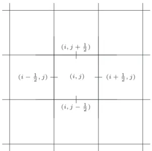
that are attached to the structure, withUdenoting the Lagrangian coordinate domain; and let𝛘(X,t) ∈ Ωdenote the physical position of material pointXat timet. The physical region occupied by the structure at timetis𝛘(U,t)⊆Ω, and the physical region occupied by the fluid at timetisΩ∖𝛘(U,t). See Figure 1. We do not assume that the Lagrangian coordinates are the initial coordinates of the elastic structure nor, more generally, do we require thatU⊆Ω.
To use a Eulerian description of the fluid and a Lagrangian description of the elasticity of the immersed structure, it is necessary to describe the stress of the fluid-structure system in both Eulerian and Lagrangian forms. Let𝝈(x,t)denote the Cauchy stress tensor of thecoupled fluid-structure system. In the present formulation, we assume that
𝝈(x,t) =𝝈f(x,t) +
{
𝝈e(x,t) forx∈𝛘(U,t),
FIGURE 1 Lagrangian and Eulerian coordinate systems. The Lagrangian material coordinate domain isU, and the Eulerian physical coordinate domain isΩ. The physical position of material pointXat timetis𝛘(X,t), the physical region occupied by the structure is𝛘(U,t), and the physical region occupied by the fluid isΩ∖𝛘(U,t)
in which𝝈f(x,t)is the stress tensor of a viscous incompressible fluid and𝝈e(x,t)is the stress tensor that describes the elastic response of the immersed structure. The fluid stress tensor is the usual one for a viscous incompressible fluid,
𝝈f(x,t) = −p(x,t)I+𝜇[∇u(x,t) + (∇u(x,t))T], (2)
in whichp(x,t)is the pressure,Iis the identify tensor,𝜇is the dynamic viscosity, andu(x,t)is the Eulerian velocity field. To describe the elasticity of the structure with respect to the Lagrangian material coordinate system, we use the first Piola-Kirchhoff elastic stress tensorPe(X,t), which is defined in terms of𝝈evia
Pe(X,t) =J(X,t)𝝈e(𝛘(X,t),t)F−T(X,t), (3) in which the deformation gradient tensor associated with the deformation𝛘∶ (U,t)→Ωis
F(X,t) = 𝜕𝛘
𝜕X(X,t), (4)
andJ(X,t) =det(F(X,t))is the Jacobian determinant of the deformation gradient. AlthoughPeis only defined within the solid region, it is convenient to extend𝝈e(x,t)by zero in the fluid region.
For simplicity, we primarily restrict our attention to hyperelastic constitutive models, which may be characterized by a strain-energy functionalWe(F). For such constitutive laws,
Pe= 𝜕We
𝜕F . (5)
Our formulation does not rely on the existence of such an energy functional, however, and it permits a material description defined only in terms of a stress response. For instance, separate work using the present methodology relies on this feature to treat active tension generation in dynamic models of muscle contraction.45-48
2.1.1
Strong formulation
As shown by Boffi et al,37the strong form of the equations of motion is
𝜌Du
Dt(x,t) = −∇p(x,t) +𝜇∇
2u(x,t) +fe(x,t), (6)
∇ ·u(x,t) =0, (7)
fe(x,t) =
∫U
∇X·Pe(X,t)𝛿(x−𝛘(X,t))dX− ∫𝜕U
Pe(X,t)N(X)𝛿(x−𝛘(X,t))dA(X), (8)
𝜕𝛘
𝜕t(X,t) =∫Ω
in which𝜌is the mass density of the coupled fluid-structure system, Du Dt(x,t) =
𝜕u
𝜕t(x,t) +u(x,t) · ∇u(x,t)is the material
derivative,fe(x,t)is the Eulerian elastic force density, and𝛿(x) =∏di=1𝛿(xi)is thed-dimensional delta function.
Two different types of Lagrangian elastic force densities appear in these equations. The Lagrangianinternal force density,
∇X·Pe, is a volumetric force density that is distributed throughout the elastic body, whereas the Lagrangiantransmission force density,−PeN, is a surface force density that is distributed along the fluid-solid interface. Equation 8 generates a corresponding Eulerian description of the elastic forces from the volumetric and surface forces. Notice thatfe(x,t)will generally have a𝛿-layer of force along the fluid-solid interface. It is possible to show thatfeis variationally equivalent to∇ ·𝝈e(for instance, by integrat-ing against a test function). Dointegrat-ing so, it is clear thatfeis singular along the fluid-solid interface wherever𝝈enis discontinuous. Indeed, because elastic stresses are present only within the structure,𝝈enis generally discontinuous at the fluid-structure inter-face. These discontinuities must be exactly balanced by discontinuities in𝝈fnto ensure that thetotalstress,𝝈=𝝈f+𝝈e, has a continuous traction vector. IfPe(X,t)is sufficiently smooth, the internal force acts as a regular (ie, nonsingular) body force and may be treated with higher-order accuracy by the IB method.37,49However, the transmission force always acts as a singular
force layer, and although this force will induce jumps in the pressure and shear stress along𝜕𝛘(U,t), such force layers may also be readily treated by the IB method.
An integral transform is also used in Equation 9 to determine the velocity of the immersed elastic structure from the material velocity fieldu(x,t). The defining property of𝛿(x)implies that Equation 9 is equivalent to
𝜕𝛘
𝜕t(X,t) =u(𝛘(X,t),t), (10)
which may be interpreted as the no-slip and no-penetration conditions of a viscous incompressible fluid. Notice, however, that the no-slip and no-penetration conditions do not appear as constraints on the fluid motion. Instead, these conditions determine the motion of the immersed structure.
2.1.2
Weak formulations
To use standard nodal (C0) FE methods for nonlinear elasticity with the IB formulation, it is necessary to introduce a weak for-mulation of the equations of motion. Here, we consider two different forfor-mulations that each uses a weak form of the Lagrangian equations. Because we use a finite difference scheme to approximate the incompressible Navier-Stokes equations, we do not develop a weak formulation for the Eulerian equations or the equations of Lagrangian-Eulerian interaction.
We begin with thepartitioned weak formulationof the equations. To do so, we first define the internal elastic force density, F(X,t), that is variationally equivalent to∇X·Peby requiring
∫U
F(X,t) ·V(X)dX= −
∫U
Pe(X,t) ∶ ∇
XV(X)dX+ ∫𝜕U
(Pe(X,t)N(X)) ·V(X)dA(X) (11)
to hold for arbitrary smoothV(X). Integrating by parts, it is clear that Equation 11 implies that
∫U
F(X,t) ·V(X)dX=
∫U
(∇X·Pe(X,t)) ·V(X)dX, (12)
for all smoothV(X). Assuming sufficient regularity,F = ∇X·Pepointwise. It is also convenient to define the transmission force density,T(X,t), pointwise along𝜕Uvia
T(X,t) = −Pe(X,t)N(X). (13)
WithFandTso defined, the equations of motion become
𝜌Du
Dt(x,t) = −∇p(x,t) +𝜇∇
2u(x,t) +f(x,t) +t(x,t), (14)
∇ ·u(x,t) =0, (15)
f(x,t) =
∫U
t(x,t) =
∫𝜕U
T(X,t)𝛿(x−𝛘(X,t))dA(X), (17)
𝜕𝛘
𝜕t(X,t) =∫Ωu(x,t)𝛿(x−𝛘(X,t))dx, (18)
in whichf(x,t)is the Eulerian internal elastic force density andt(x,t)is the Eulerian transmission elastic force density. It is important to notice that, under relatively mild regularity requirements,FandTare both smooth functions on their domains of definition, andfis piecewise smooth. Under these conditions, the only singular function in this formulation ist.
Alternative weak definitions of the Lagrangian elastic force density are possible. The formulation typically used with the IFE method defines atotalelastic force per unit volume,G(X,t), by requiring
∫U
G(X,t) ·V(X)dX= −
∫U
Pe(X,t) ∶ ∇
XV(X)dX (19)
for arbitraryV(X). It is possible to see thatG(X,t)accounts for the effects ofboththe internal and transmission force densities of the strong form of the equations. To do so, we again integrate by parts to find that
∫U
G(X,t) ·V(X)dX=
∫U
(∇ ·Pe(X,t)) ·V(X)dX−
∫𝜕U
(Pe(X,t)N(X)) ·V(X)dA(X), (20) for allV(X). Thus,G(X,t)can be a continuous function only ifPeN≡ 0. In general,Gis in fact a distribution that accounts for both the internal force per unit volume and the transmission force per unit area, in which the transmission force gives rise to a singular force layer concentrated along𝜕U. It is possible to use Equation 19 with standard finite element methods; however, when doing so, the transmission surface force density is effectively projected (in anL2sense) onto the volumetric basis functions. Specifically, the FE basis functions serve toregularizethe transmission force.
Using this definition ofG, we may state aunified weak formulationthat includes only a single, unified body forcing term:
𝜌Du
Dt(x,t) = −∇p(x,t) +𝜇∇
2u(x,t) +g(x,t), (21)
∇ ·u(x,t) =0, (22)
g(x,t) =
∫U
G(X,t)𝛿(x−𝛘(X,t))dX, (23)
𝜕𝛘
𝜕t(X,t) =∫Ω
u(x,t)𝛿(x−𝛘(X,t))dx, (24)
in whichg(x,t)is the Eulerian total elastic force density. This weak form of the equations of motion is essentially the formulation used in the IFE method,30-34the energy-based formulation of Devendran and Peskin,35,36and the fully variational IB method.37-39
To our knowledge, the partitioned formulation described here has not been widely used in previous work.
2.2
Immersed rigid structures
The equations of motion for a fixed, rigid structure are similar to those used in the case of an immersed elastic structure:
𝜌Du
Dt(x,t) = −∇p(x,t) +𝜇∇
2u(x,t) +f(x,t), (25)
∇ ·u(x,t) =0, (26)
f(x,t) =
∫U
𝜕𝛘
𝜕t(X,t) =∫Ωu(x,t)𝛿(x−𝛘(X,t))dx=0, (28)
in which here,F(X,t)is a Lagrange multiplier for the constraint 𝜕𝜕𝛘t ≡0. Thus, this fully constrained formulation takes the form of an extended saddle-point problem with two Lagrange multipliers,p(x,t)for the incompressibility constraint andF(X,t)for the rigidity constraint. Solving this system effectively requires specialized techniques that are the subject of active research.43,44
In this work, we consider instead a penalty formulation for an immersed stationary structure, in which the Lagrange multiplier force is approximated by
F(X,t) =𝜅(𝛘(X,0) −𝛘(X,t)) −𝜂𝜕𝛘
𝜕t(X,t), (29)
in which𝜅 ⩾ 0 is a stiffness penalty parameter and𝜂 ⩾ 0 is a damping penalty parameter. As𝜅 → ∞,𝛘(X,t) → 𝛘(X,0), and𝜕𝛘
𝜕t →0, so that this formulation is equivalent to the constrained formulation. In principle, it is not necessary to include the
damping parameter𝜂; however, we have found that using damping reduces numerical oscillations, especially at moderate-to-high Reynolds numbers.
3
S P A T I A L D I S C R E T I Z A T I O N
For simplicity, we describe the numerical scheme in two spatial dimensions. The extension of the numerical scheme to the case d=3 is straightforward.
3.1
Eulerian discretization
We use a staggered-grid finite difference scheme to discretize the incompressible Navier-Stokes equations in space. Compared to collocated discretizations (ie, purely cell- or node-centered schemes), such Eulerian discretization approaches yield superior accuracy when used with the conventional IB method.50 To simplify the exposition, assume thatΩis the unit square and is
discretized using a regularN×NCartesian grid with grid spacings Δx1 = Δx2 = h = N1. Let (i,j)label the individual Cartesian grid cells for integer values ofiandj, 0⩽ i,j< N. The components of the Eulerian velocity fieldu = (u1,u2)are approximated at the centers of thex1- andx2-edges of the Cartesian grid cells, ie, at positionsxi−12,j =
(
ih,(j+1
2 )
h)and
xi,j−1 2 =
(( i+1
2 )
h,jh )
, respectively. A staggered scheme is also used for the Eulerian body forcef = (f1,f2). We use the notation(u1)i−12,j,(u2)i,j−12,(f1)i−12,j, and(f2)i,j−12 to denote the discrete values ofuandf. The pressurepis approximated at the
centers of the Cartesian grid cells, and its discrete values are denotedpi,j. See Figure 2.
Let∇h·u≈ ∇ ·u,∇hp≈ ∇p, and∇2hu≈ ∇2urespectively denote standard second-order accurate finite difference
approx-imations to the divergence, gradient, and Laplace operators.51In this approach,∇
h·uis defined at cell centers, whereas both ∇hpand∇2huare defined at cell edges. We use a staggered-grid version50,51of the xsPPM7 variant52of the piecewise parabolic
method (PPM)53to discretize the nonlinear advection terms. Where needed, physical boundary conditions are discretized and
imposed along𝜕Ωas described by Griffith.51In some numerical examples, we use a locally refined Eulerian discretization that
uses Cartesian grid adaptive mesh refinement (AMR) following the discretization approach described by Griffith.26
3.1.1
Eulerian inner products
Ifuandvare discrete staggered-grid vector fields, we denote by[u]and[v]the corresponding vectors of grid values. IfΩhas periodic boundaries, we define the discreteL2inner product onΩby
(u,v)x= [u]T[v]h2. (30)
Minor adjustments to this definition are required when nonperiodic physical boundary conditions are used51or near coarse-fine
FIGURE 2 Schematic of the staggered-grid layout of Eulerian degrees of freedom in 2 spatial dimensions. The pressures are approximated at cell centers, indicated by(i,j), thex1-components of the velocity and force are approximated on thex1-edges,(i−12,j)or(i+12,j), and the
x2-components of the velocity and force are approximated on thex2-edges,(i,j− 1
2)or(i,j+ 1 2)
3.2
Lagrangian discretization
Leth = ∪eUebe a triangulation ofUcomposed of elementsUe, in whicheindexes the elements of the mesh. We denote by {Xl}Ml=1the nodes of the mesh, and by{𝜙l(X)}Ml=1nodal (Lagrangian) FE basis functions. The time-dependent physical positions
of the nodes of the Lagrangian mesh are{𝛘l(t)}Ml=1, and using the FE basis functions, we define an approximation to𝛘(X,t)by
𝛘h(X,t) = M
∑
l=1
𝛘l(t)𝜙l(X). (31)
An approximation to the deformation gradient is given by
Fh(X,t) = 𝜕𝛘h 𝜕X(X,t) =
M
∑
l=1
𝛘l(t) 𝜕𝜙 l
𝜕X(X). (32)
3.2.1
Immersed elastic structures
For an immersed elastic structure, we use the FE approximation to the deformation gradient tensorFh(X,t)to computePeh(X,t)
andTh(X,t), which are approximations to the first Piola-Kirchhoff stress tensor and the Lagrangian transmission force density,
respectively. We approximate the Lagrangian force densitiesF(X,t)andG(X,t)by
Fh(X,t) = M
∑
l=1
Fl(t)𝜙l(X), and (33)
Gh(X,t) = M
∑
l=1
Gl(t)𝜙l(X). (34)
The nodal values{Fl}Ml=1and{Gl}Ml=1must be determined fromPeh(X,t)via discretizations of Equation 11 and Equation 19. We
use a standard Galerkin approach, so that after rearranging terms, Equation 11 becomes
M
∑
l=1 (
∫U
𝜙l(X)𝜙m(X)dX
)
Fl(t) = −
∫U
Pe
h(X,t) ∇X𝜙m(X)dX+
∫𝜕U
Pe
for eachm=1,…,M. Similarly, Equation 19 becomes
M
∑
l=1 (
∫U
𝜙l(X)𝜙m(X)dX
)
Gl(t) = −
∫U
Pe
h(X,t) ∇X𝜙m(X)dX, (36)
for eachm=1,…,M. In practice, these integrals are approximated via Gaussian quadrature.
3.2.2
Immersed rigid structures
For a fixed, rigid immersed structure, we directly evaluate the discretized Lagrangian penalty forceFh(X,t)via
Fh(X,t) =𝜅
(
𝛘h(X,0) −𝛘h(X,t)
)
−𝜂𝜕𝛘h
𝜕t (X,t). (37)
Because𝛘h(X,t)andFh(X,t)are defined in terms of the same basis functions,Fh(X,t)is given by
Fh(X,t) =
∑
l
Fl(t)𝜙l(X) (38)
in which
Fl(t) =𝜅
(
𝛘l(0) −𝛘l(t)
)
−𝜂d𝛘l
dt (t). (39)
3.2.3
Lagrangian inner products
Letting[F]denote the vector of nodal coefficients ofFh, we write Equation 35 as
[] [F] = [B], (40)
in which[]is the mass matrix that has entries of the form ∫U𝜙l(X)𝜙m(X)dX. Equation 36 may be rewritten similarly.
The mass matrix[]can also be used to evaluate theL2inner product of Lagrangian functions onU. In particular, for any Uh(X,t) =∑lUl(t)𝜙l(X)andVh(X,t) =∑lVl(t)𝜙l(s),
(Uh,Vh)X= [U]T [] [V]. (41)
Different choices of mass matrices (eg, lumped mass matrices) induce different discrete inner products onU.
To simplify notation, in the remainder of this paper, we drop the subscript hfrom our numerical approximations to the Lagrangian variables.
3.3
Lagrangian-Eulerian interaction
We next describe Lagrangian-Eulerian coupling operators that take advantage of the kinematic information encoded in the FE approximation to the deformation of the immersed structure. As in the conventional IB method, we approximate the singular delta function kernel appearing in the Lagrangian-Eulerian interaction equations by a smoothedd-dimensional Dirac delta function𝛿h(x)that is of the tensor-product form𝛿h(x) =∏
d
i=1𝛿h(xi). Except where otherwise noted, in this work, we take the
one-dimensional smoothed delta function𝛿h(x)to be the four-point delta function of Peskin.3
To compute an approximation to f = (f1,f2)on the Cartesian grid, we construct for each elementUe ∈
h a Gaussian
quadrature rule withNequadrature pointsXeQ∈Ueand weights𝜔e
Q,Q=1,…,N e
(f1)i−1 2,j
= ∑
Ue∈ h
Ne
∑
Q=1
F1(XeQ,t)𝛿h
( xi−1
2,j
−𝛘(XeQ,t))𝜔eQ, and (42)
(f2)i,j−1 2
= ∑
Ue∈ h
Ne
∑
Q=1
F2(XeQ,t)𝛿h
( xi,j−1
2
−𝛘(XeQ,t))𝜔eQ, (43)
withF(X,t) = (F1(X,t),F2(X,t)). We use the notation
f(x,t) =(𝛘(·,t)) F(X,t), (44)
in which(𝛘(·,t))is theforce-prolongation operatorimplicitly defined by Equations 42 and 43. Notice that
(f1)i−1 2,j
= ∑
Ue∈ h∫U
e
F1(X,t)𝛿h
( xi−1
2,j
−𝛘(X,t))dX+O(ΔXq), and (45)
(f2)i,j−12 =
∑
Ue∈ h∫U
e
F2(X,t)𝛿h
( xi,j−1
2
−𝛘(X,t))dX+O(ΔXq), (46)
in whichΔXis proportional to the Lagrangian mesh spacing andO(ΔXq)corresponds to quadrature error that may be controlled by the choice of numerical quadrature rules.
A correspondingvelocity-restriction operator (𝛘(·,t))determines the motion of the nodes of the Lagrangian mesh from the Cartesian grid velocity field via
𝜕𝛘
𝜕t(X,t) = (𝛘(·,t)) u(x,t). (47)
There are many possible ways to construct; however, we have found that an effective approach is to require 𝜕𝛘
𝜕t = uto
satisfy the discrete power identity,
( F,𝜕𝛘
𝜕t )
X
= (f,u)x, (48)
which implies that the semidiscrete unified formulation conserves energy during Lagrangian-Eulerian interaction.3This power
identity can be rewritten as
(F, u)X= (F,u)x, (49)
ie, =∗.
To construct explicitly, it is convenient to use matrix notation. Identifying[]and[ ]with the matrix representations of and, we have that
[f] = [] [F]and (50)
d[𝛘]
dt = [ ] [u]. (51)
Equation 49 then becomes
[F]T [] [ ] [u] = ([] [F])T [u]h2. (52)
[ ] = []−1[]T h2. (53) In our time-stepping scheme, which is stated below in Appendix A.1, notice that we need only to apply[ ]to discrete velocity fields defined on the Cartesian grid. Specifically, we do not need to compute[ ]explicitly.
It is straightforward to show that this construction of implies that𝜕𝛘
𝜕t(X,t)is an approximation to theL
2projection of the Lagrangian vector fieldUIB(X,t) = (UIB
1 (X,t),U IB
2 (X,t)), with U1IB(X,t) =∑
i,j
(u1)i−12,j 𝛿h
( xi−1
2,j−𝛘(
X,t))h2, and (54)
U2IB(X,t) =∑ i,j
(u2)i,j−12 𝛿h
( xi,j−1
2
−𝛘(X,t))h2. (55)
Because the components ofUIB(X,t)are not generally linear combinations of the FE basis functions, generally 𝜕𝛘
𝜕t ≠U
IB. For the semidiscretized partitioned formulation,fis computed on the Cartesian grid viaf=F. The Eulerian transmission force densitytis computed in a similar manner, but in this case, the numerical integration occurs only over those element boundaries that coincide with𝜕U. We use the notationt=𝜕UTto denote this operation. We use the same regularized delta
function𝛿h(x)to construct bothand𝜕U. For simplicity, we use the same velocity-restriction operator for both formulations.
This choice ensures that the 2 formulations coincide wheneverT≡0.
The Lagrangian-Eulerian interaction operators introduced in this work are different from analogous operators generally used in standard IB methods. Standard IB methods and schemes such as the IFE method use regularized delta functions to apply nodal forces directly to the Cartesian grid and to interpolate Cartesian grid velocities directly to the Lagrangian nodes.3In such
schemes,f(x,t)would be approximated on the Eulerian grid by expressions similar to
( f1IB)i−1
2,j
= M
∑
l=1
(F1)l(t)𝛿h
( xi−1
2,j
−𝛘l(t)
)
𝜔IB
l ,and (56)
( f2IB)i,j−1
2
= M
∑
l=1
(F2)l(t)𝛿h
( xi,j−1
2 −𝛘l(t)
)
𝜔IB
l , (57)
in whichfIB denotes the Eulerian force determined by the standard IB force-spreading operator and𝜔IB
l denotes the volume
associated with Lagrangian nodel. In this approach, each nodal forceFlis applied only to Cartesian grid cells within the support
of𝛿h(x−𝛘l), and the Lagrangian mesh must therefore be finer than the Cartesian grid to avoid leaks.3The corresponding
approach to velocity restriction used by such methods would be to setd𝛘l
dt =U
IB(X
l,t).
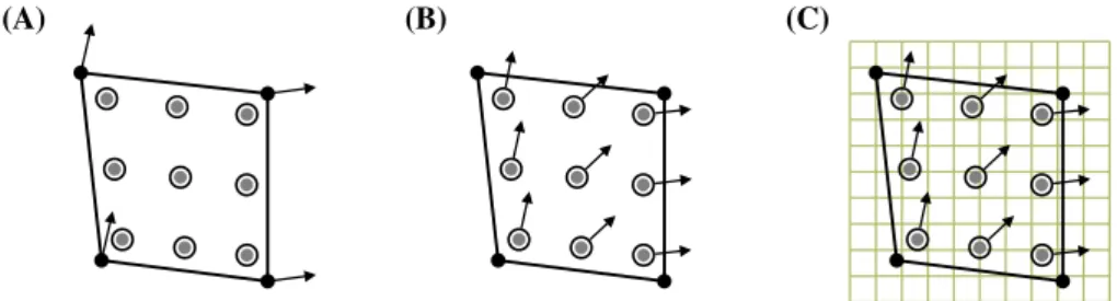
Our Lagrangian-Eulerian interaction operators communicate between a collection of Lagrangian control points (the nodes of the structural mesh) and the Cartesian grid via a collection of interaction points (the Lagrangian quadrature points). The force-prolongation operator can be seen as the composition of 2 operations: First, the Lagrangian force density is evaluated at the interaction points in terms of data defined at the control points; then the standard IB delta function𝛿h(x)spreads volume- or
area-weighted force densities from the interaction points to the Cartesian grid. See Figure 3. Velocity restriction is similar: First, the Cartesian velocity field is interpolated to the interaction points using𝛿h(x); then these velocities are accumulated to form
the right-hand side of a system of equations that determines𝜕𝛘
𝜕t at the control points. Our approach is similar to methods used
in RBF-based IB methods.42
In general, it is necessary that the same interaction points are used in the discrete force-spreading and velocity-interpolation operators if those operators are to satisfy a discrete adjoint property. It is possible to construct an interpolation operator that uses the control points as the interaction points, but then satisfying the discrete adjoint property requires that the control points are also used as the interaction points in the spreading operator.
FIGURE 3 Prolonging the elastic force density from the Lagrangian mesh onto the Eulerian grid. Starting with an approximation to the force density at the nodes of the Lagrangian mesh A, we use the interpolatory FE basis functions to determine the force density at interaction points that are defined by a quadrature rule B, and then spread those forces from the interaction points to the background Eulerian grid using the smoothed delta function𝛿h(x)C. This approach permits Lagrangian meshes that are significantly coarser than the Eulerian grid so long as the “net” of interaction points is sufficiently dense. Denser nets of interaction points can be obtained, for instance, by increasing the order of the numerical quadrature scheme
4
I M P L E M E N T A T I O N
This version of the IB method is implemented in the open-source IBAMR software,54which is a C++ framework for developing
FSI models that use the IB method. The IBAMR provides support for distributed-memory parallelism and AMR. The IBAMR relies upon the SAMRAI,55-57PETSc,58-60hypre,61,62andlibMesh63,64libraries for much of its functionality.
5
N U M E R I C A L R E S U L T S
5.1
Thick elliptical shell
This section presents results from tests that use a thick elastic shell23,37,49 to demonstrate the convergence properties of our
method for different types of material models.
In these computations, the physical domain isΩ = [0,1] × [0,1]with periodic boundary conditions, and following Boffi et al,37 the Lagrangian coordinate domainUis defined using curvilinear coordinatess = (s
1,s2) ∈ Uinstead of reference coordinates, withU= [0,2𝜋R] × [0,w]forR=0.25 andw=0.0625, and with periodic boundary conditions in thes1direction. The coordinate mapping𝛘∶ (U,t)→Ωis given at timet=0 by
𝛘(s,0) = (cos(s1∕R)(R+s2) +0.5,sin(s1∕R)(R+𝛾+s2) +0.5). (58)
For𝛾 =0, the initial configuration of the shell is a circular annulus with inner radiusRand thicknessw, which corresponds to an equilibrium configuration of the structure. For𝛾 ≠0, the initial configuration is an elliptical annulus that is out of equilibrium. In our tests, we use𝛾 =0 for static problems and𝛾 =0.15 for dynamic problems. In either case, we discretizeΩusing anN-by-N Cartesian grid. The Lagrangian discretization is constructed so that the nodes of the Lagrangian mesh are physically separated by a distance of approximatelyMfacΔx. Specifically, we discretizeUusing a 28M-by-Mmesh of bilinear (Q1) elements, with M= M1
fac N
16. Representative numerical results usingN=128 are shown in Figures 4 and 7.
Although this is a relatively simple benchmark problem, the static version (𝛾 =0) is one of the only test problems available for the IB method that we know of that permits a simple analytic solution. Moreover, because certain choices ofPeallow the IB method to attain higher-order convergence rates, this test case allows us to verify that our implementation attains its designed order of accuracy.
5.1.1
Anisotropic shell
We first consider an idealized anisotropic material model defined in terms of
We(F) = 𝜇
e 2w‖‖‖‖
𝜕𝛘
𝜕s1‖‖‖‖ 2
= 𝜇
e
2wF𝛼1F𝛼1, (59)
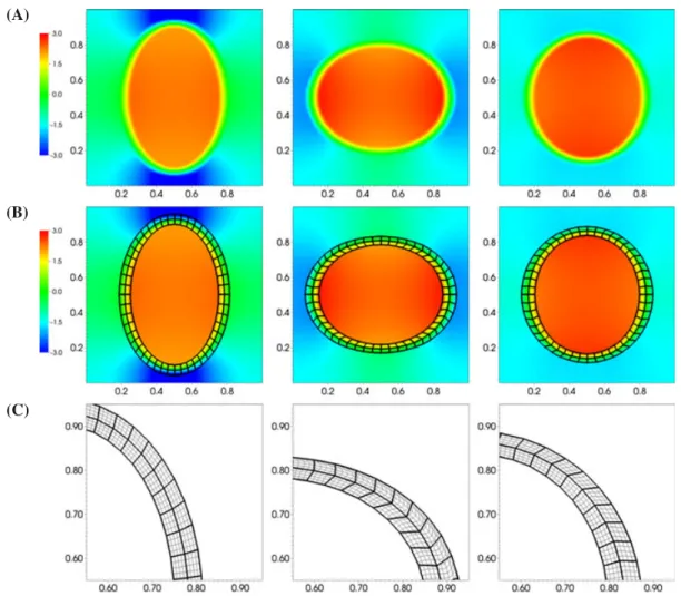
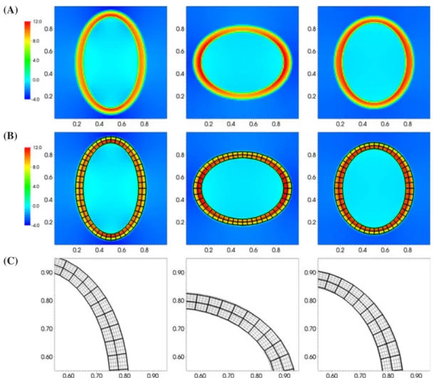
FIGURE 4 Representative results from the dynamic (𝛾=0.15) version of the idealized anisotropic shell model of Section 5.1.1 forN=128 over the time interval 0⩽t⩽0.75. The computed pressure and structure deformation forMfac=4 are shown in A and B. The computed deformations
obtained withMfac=1 andMfac=4 are compared in C. The coarse and fine structural meshes yield essentially identical kinematics
Pe= 𝜕We
𝜕F = 𝜇 e w
(𝜕𝛘1
𝜕s1
0
𝜕𝛘2 𝜕s1 0
)
= 𝜇
e w
( F11 0 F21 0
)
. (60)
This model corresponds to an idealized elastic material composed of a continuous family of extension-resistant fibers that wrap the thick shell. BecauseUis periodic in thes1 direction,PeN ≡ 0 along𝜕U. If we view the structure as a fiber-reinforced material, none of the fibers terminate along the boundary of the structure. Because the transmission force vanishes in this case, the unified and partitioned weak formulations are identical.
Setting𝛾 =0, so that the structure is in equilibrium, and requiring∫Ωp(x,t)dx=0, it can be shown37that
p(x,t) =
⎧ ⎪ ⎨ ⎪ ⎩
p0+𝜇Re r⩽R,
p0+𝜇we1R(R+w−r) R<r⩽R+w, p0 R+w<r,
(61)
withr = ||x− (0.5,0.5)||andp0 = 𝜋𝜇e
3w
(
R2− (R+Rw)3
)
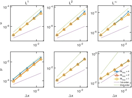
. We set𝜌 = 1,𝜇= 1, and𝜇e = 1, and we consider the time interval 0⩽t⩽3. Figure 5 summarizes the error data at timet=3 forN=64, 128, 256, 512, and 1024, usingMfac=1, 2, and 4, with
Δt = 0.25Δx. Second-order convergence rates are observed in theL1,L2, andL∞norms for the velocity field. Second-order
convergence rates are also observed for the pressure in theL1norm; however, because the pressure field isC0but notC1, only first-order convergence rates are observed for the pressure in theL∞norm, and intermediate convergence rates (approximately
FIGURE 5 Errors inuandpinL1,L2, andL∞norms for the static (𝛾=0) version of the idealized anisotropic shell model of Section 5.1.1. Reference lines with slopes of -1 and -2 are also shown. The velocity converges at second-order accuracy in all norms, whereas the pressure converges at second-order in theL1norm, at first-order in theL∞norm, and at order 1.5 in theL2norm
We also consider the case in which𝛾 =0.15, so that the initial configuration of the shell is not in equilibrium. We set𝜌=1,
𝜇= 0.01, and𝜇e= 1, yielding a Reynolds number of approximately 50. We consider the time interval 0 ⩽t ⩽ 0.75, which corresponds to approximately one damped oscillation of the shell. Because an exact solution is not available in this case, we use a Richardson extrapolation approach, as described in detail in previous work.49Figure 6 summarizes the error data at time
t = 0.75 forN = 64, 128, 256, and 512 and Mfac = 1, 2, and 4, withΔt = 0.25Δx. Essentially second-order convergence rates are observed in theL1,L2, andL∞norms for the velocity field. The pressure converges at a second-order rate in theL1 norm, at a first-order rate in theL∞norm, and at an intermediate rate (approximately 1.5) in theL2norm. Convergence rates for the deformation are somewhat less regular, with nearly second-order convergence rates being observed in theL1andL2norms and between first- and second-order convergence rates observed in theL∞norm. The robustness of the convergence rate in the deformation can be improved by using higher-order structural elements. Because the overall accuracy of the discretization is also limited by the Eulerian discretization and the form of the regularized kernel function, however, the use of higher-order elements does not in itself increase the overall order of accuracy of the method.
Notice that in both the static and dynamic test cases, virtually identical errors are attained for all of the values ofMfac con-sidered. This indicates that for these tests, the method is able to use relatively coarse structural meshes without appreciable loss in accuracy. In particular, these results suggest that the scheme does not allow leaks at fluid-structure interfaces, even for Lagrangian meshes that are quite coarse compared to the Eulerian grid.
5.1.2
Orthotropic shell
The second case that we consider uses a neo-Hookean material model,
We(F) = 𝜇
e
2wI1(C), (62)
withC=FTFandI
1(C) =tr(C), so that
Pe= 𝜇e
wF. (63)
FIGURE 6 Errors inu,p, and𝛘inL1,L2, andL∞norms for the dynamic (𝛾=0.15) version of the idealized anisotropic shell model of Section 5.1.1. Reference lines with slopes of -1 and -2 are also shown. The velocity converges at second-order accuracy in all norms, whereas the pressure converges at second-order in theL1norm, at first-order in theL∞norm, and at order 1.5 in theL2
norm. The displacement converges at essentially second-order rates in theL1andL2norms, and at a slightly lower rate in theL∞norm
fluid-structure interfaces, there are singular force layers along𝜕𝛘(U,t)that must be balanced by discontinuities in the pressure and viscous stress. Therefore, in this case, the discretized unified and partitioned formulations yield different results.
Setting𝛾 =0, so that the structure is in equilibrium, and requiring∫Ωp(x,t)dx=0, it can be shown37that
p(x,t) =
⎧ ⎪ ⎨ ⎪ ⎩
p0+𝜇e(1
R−
1
R+w
)
r⩽R,
p0+ 𝜇we
( 1
R(R+w−r) + R R+w
)
R<r⩽R+w,
p0 R+w<r,
(64)
withr = ||x− (0.5,0.5)||andp0 = 𝜋𝜇e
3w
(
3wR+R2− (R+Rw)3
)
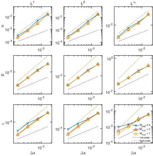
. We set𝜌 = 1,𝜇 = 1, and𝜇e = 1, and we consider the time interval 0⩽ t⩽3. Figure 8 summarizes the error data at timet= 3 forN=64, 128, 256, 512, and 1024, usingMfac =1, 2, and 4, withΔt=0.25Δx. First-order convergence rates are observed foruin all norms. First-order convergence rates are also observed forpin theL1 norm. Becauseppossesses discontinuities at fluid-structure interfaces for this problem; however, the present method yields convergence rates of 0.5 in theL2norm and does not converge in theL∞norm.
We also consider the case in which𝛾 =0.15, so that the initial configuration of the shell is not in equilibrium. We set𝜌=1,
𝜇=0.01, and𝜇e =1, yielding a Reynolds number of approximately 100. We consider the time interval 0⩽ t⩽1.25, which corresponds to approximately one damped oscillation of the shell. Again, an exact solution is not available, and so convergence rates are estimated using Richardson extrapolation.49Figure 9 summarizes the error data at timet=0.75 forN=64, 128, 256,
and 512 andMfac=1 and 4, withΔt=0.25Δx. Essentially first-order convergence rates are observed foruand𝛘in all norms, whereaspexhibits first-order convergence in only theL1norm.
FIGURE 7 Similar to Figure 4, but here, showing results obtained using the orthotropic shell model of Section 5.1.2 forN=128 and the partitioned (split) weak formulation over the time interval 0⩽t⩽1.25. As in Figure 4, the coarse and fine structural meshes yield very similar kinematics
𝛘. By contrast, the partitioned formulation offers significantly better accuracy for the pressure for relatively coarse Lagrangian meshes. This property appears also to result in improvements in volume conservation; see Section 5.2.
5.2
Soft elastic disc in lid driven cavity
This section presents results from tests that use a soft elastic structure in a lid-driven cavity flow to demonstrate the volume-conservation properties of our method.
In these computations, the physical domain isΩ = [0,1] × [0,1], and the immersed structure is a disc of radius 0.2 that is initially centered aboutx= (0.6,0.5). The boundary conditions imposed along𝜕Ωareu≡0 on the left (x1=0), right (x1=1), and bottom (x2=0) boundaries ofΩ, andu≡(1,0)on the top (x2=1) boundary ofΩ. We use an isotropic neo-Hookean model,
Pe=𝜇eF−p0F−T, (65)
and we consider bothp0 = 0 andp0 = 𝜇e. Because generallyPeN≢ 0, the solution has discontinuities in the pressure and viscous stress at fluid-structure interfaces. In such cases, we expect the IB method to yield no better than first-order convergence rates.†The flow induced by the driven lid brings the structure nearly into contact with the moving upper boundary of the domain; see Figure 10. This near contact is handled automatically by the IB formulation using a version of a modified kernel function approach introduced by Griffith et al24and enhanced by Kallemov et al.43No additional specialized methods are required by
the present scheme to handle this case.
†This flow also possesses well-known corner singularities that reduce the convergence rate of the incompressible flow solver. Although it is possible to devise
FIGURE 8 Errors inuandpinL1,L2, andL∞norms for the static (𝛾=0) version of the orthotropic shell model of Section 5.1.2. Errors for the unified formulation appear as solid lines, and errors for the partitioned formulation appear as dashed lines. Reference lines with slope -1 are provided for theuerror data. Forp, reference lines with slopes -1 and -0.5 are provided for theL1andL2norm data, respectively. Because this test includes discontinuities in the pressure at fluid-structure interfaces, the present method does not yield convergence inpin theL∞norm. The partitioned formulation generally yields improved accuracy compared to the unified formulation, especially for the pressure for relatively coarse structural mesh spacings
As in previous studies of this test case,33,66 we set𝜇 = 0.01 and𝜌= 1. We consider𝜇e = 0.2, which is a relatively “soft” case. The initial velocity isu≡0, and the reference coordinatesXare taken to be the initial coordinates, so that𝛘(X,0)≡X. The physical domain is discretized using anN×NCartesian grid. The Lagrangian coordinate domain is discretized using an unstructured mesh of quadratic triangular (P2) elements constructed so that the elements are approximately a factor of Mfaccoarser than the background Eulerian grid, so that in the reference configuration, the nodes of the Lagrangian mesh are physically separated by a distance of approximatelyMfacΔx. The time step size isΔt=0.125Δx. We consider the time interval 0 ⩽ t ⩽ 10, during which the disc is subjected to slightly more than one rotation within the cavity. The structure becomes entrained in the shearing flow along the cavity lid fromt ≈ 4 until t ≈ 6 and during this time is subjected to very large deformations. Figure 11 shows the percent change in disc volume for different values ofNandMfac. Withp0=0, the maximum volume change yielded by the unified formulation is approximately 2.3% forN = 64 andMfac = 4, 0.4% for N = 64 and Mfac = 2, and 0.2% forN = 64 andMfac = 1. The split formulation yields substantially improved accuracy: The maximum volume change is approximately 0.12% forN = 64 andMfac = 4, 0.2% forN = 64 andMfac = 2, and 0.15% forN = 64 andMfac = 1. Setting p0 = 𝜇eimproves the accuracy of the unified formulation substantially, especially at coarser relative mesh spacings, whereas it results in slightly poorer volume conservation for the split formulation. Withp0 =𝜇e, the maximum volume change is less than 0.4% in all cases considered. At smaller values ofMfac, there is essentially no difference in the volume changes produced by the unified and partitioned formulations. In all cases, the maximum volume change converges to zero at a first-order rate.
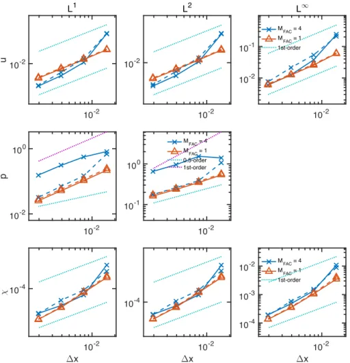
FIGURE 9 Errors inu,p, and𝛘inL1,L2, andL∞norms for the dynamic (𝛾=0.15) version of the orthotropic shell model of Section 5.1.2. Errors for the unified formulation appear as solid lines, and errors for the partitioned formulation appear as dashed lines. Reference lines with slope -1 are provided for theuand𝛘error data. Forp, reference lines with slopes -1 and -0.5 are provided for theL1andL2norm data, respectively. The
unified formulation generally yields modest improvements in the accuracy foruand𝛘, whereas the partitioned formulation generally yields improved accuracy forp, especially for relatively coarse structural mesh spacings.
FIGURE 10 A soft neo-Hookean disc in a lid-driven cavity flow using the partitioned (split) weak formulation withN=128 andMfac=4 over
the time interval 3⩽t⩽7
5.3
Flow past a cylinder
This section presents results from tests using the widely used benchmark of viscous flow past a stationary circular cylinder. In these computations, the physical domain isΩ = [−15,45] × [−30,30], and the immersed structure is a thin circular interface of radius 0.5 centered aboutx = (0,0). This domain size and cylinder placement corresponds to “Case C” considered by Taira and Colonius.67Along the inflow boundary (x
1= −15), we set a uniform inflow velocity,u≡(1,0). Along the outflow boundary (x1 = 45), we set the normal traction and tangential velocity to zero, whereas along the top (x2 = 30) and bottom (x2= −30) boundaries, we set the normal velocity and tangential traction to zero. The boundary condition treatment is the same as that described by Griffith.51We set𝜌= 1 and𝜇 = 0.005. Using the inflow velocity as the characteristic velocityu
∞and
the cylinder diameterdas the characteristic length, the Reynolds number isRe= 𝜌u∞d
FIGURE 11 Percent change in structure volume for the soft elastic disc benchmark of Section 5.2 as a function of time using Equation 65 with A,p0=0 and B,p0=𝜇e. Results are shown for Cartesian grids of sizeN=64, 128, and 256 with relative Lagrangian mesh spacingsMfac=4, 2,
and 1. The amount of spurious volume change converges to zero at first order. At coarser relative mesh spacings, the partitioned (split) formulation yields substantially better volume (area in 2 spatial dimensions) conservation than the unified (unsplit) formulation. Volume conservation is substantially improved for the unified formulation by settingp0=𝜇e. The volume change is less than 0.4% for all cases considered except for the
unified formulation withp0=0 andMfac=4.
discretized using an adaptively refined Cartesian grid with six nested grid levels and a refinement ratio of two between levels. The Cartesian grid spacing on the finest grid level isΔxfinest =2−5Δxcoarsest, withΔxcoarsest = 60N. The cylinder is discretized using a mesh of one-dimensional quadratic (P2) elements with a node spacing of approximatelyMfacΔxfinest. The time step size is