ADAPTING COMMUNITY DETECTION APPROACHES TO LAGRE,
MULTILAYER, AND ATTRIBUTED NETWORKS
Natalie Stanley
A dissertation submitted to the faculty of the University of North Carolina at Chapel Hill in partial fulfillment of the requirements for the degree of Doctor of Philosophy in the Curriculum in Bioinformatics and Computational Biology.
Chapel Hill 2018
Approved by: Peter Mucha
Marc Niethammer
Jeremy Purvis
Tamara Berg
David Gotz
ABSTRACT
Natalie Stanley: Adapting community detection approaches to large, multilayer, and attributed networks (Under the direction of Peter J. Mucha)
ACKNOWLEDGEMENTS
I’m glad this is the part of the thesis that people like to read because I have many thanks to share. First, thank you to my advisor, Peter. Thank you for always treating me like a scientist and a collaborator, more than a student. I think that a trait of a great advisor is their willingness to work collaboratively with their students, and Peter does this incredibly well. Thank you for always being positive about results (even if no positivity was warranted), for providing suggestions, and for allowing me to work on whatever I wanted to. Thank you for helping me through ‘existential angst’ and for supporting me in whatever career path I wanted to take. Thank you for always making sure there was a grant to pay my salary and for all of the meetings and Slack conversations. I will always remember to ignore the gong and how one good result is already more than most of the literature. I am forever grateful for all of your support.
Next, thank you to my pseudo second advisor, Marc. Thank you for always reading my write ups and papers and for always having great questions and suggestions. I always admire how successful, creative, and humble you are (and a great sense of humor). Thank you for all of your time and Monday meetings. The Monday meetings with Peter and Roland are some of my best memories.
Thank you to Saray and Dane who have played an important role in mentoring me as a beginning grad student and helping me to write my first paper. Dane, thank you for your very detailed editing and notation considerations. I will always remember the suggestions you made on the first paper. Saray, I am so lucky to work with you and even more lucky to have you as a friend. I rarely have met people that I can communicate with through eye contact. Our entropy together made everything more fun, from yard time, to flying with the random physicist to Zaragoza and getting displaced in a tiny elevator.
I have been lucky to interact with a lot of great people over the years in the Mucha research group. Thanks to Nishant, Wayne, Sam, Howdy, Clara, Eun, Peter D, Nic, and Sean for brightening up Chapman. Thank you to the people who make BCB run- Tim Elston, Will Valdar, and John Cornett. I know you all work very hard for BCB and I think we have a great group of creative students. We all owe so much gratitude to John Cornett who is always friendly, positive, responsive, and on top of things. I am also lucky to have met great friends in BCB who I have done homework with, looked up to, and have given me great advice. Thank you, Bryan, Dan, Greg, and Paul.
Thanks to living in Chapel Hill, I was fortunate to make some incredible friends. To my super strong (literally strong) lady friends Jess, Mimi, and Libby: Thank you for all the nights we spent laughing and climbing. These are some of the best times. Thank you Andrew for being the most incredible nerd friend and one of the kindest people I have ever met. I can always count on you for awesome conversation.
Last but not least, I owe a huge amount of gratitude to my family. First to my parents Pat and Eric who have supported me every day of my life. They have never put any pressure on me to do anything and support all of my dreams unconditionally. Most importantly, they are really friendly and fun people. I couldn’t choose better parents. Thank you for tolerating my un responded text messages, my inability to mail a letter or find a stamp, and for helping me through tough times. Next to my brother, Mike (who is a statistician). I admire you so much for always following your dreams. Aside from being great at everything you do, you are such a kind, wonderful person. I hope you don’t find any mistakes in this thesis or ask about consistency.
Finally, thank you Thomas for supporting me in every possible way. I’m so happy that grad school lead me to you. You have enhanced my life in every way and inspire me every day to be a scientist. I am so lucky to have a great role model who works so hard, is so talented, and so kind. Thank you for always pushing me pursue things I didn’t think that I could. Thank you for always telling me ‘shhhh’ when I started to get stressed. You are my favorite Dub.
TABLE OF CONTENTS
LIST OF TABLES . . . xiii
LIST OF FIGURES . . . xiv
LIST OF ABBREVIATIONS . . . .xxiv
1 Introduction . . . 1
1.1 Network Notation and Basic Summarization . . . 2
1.1.1 Representing relational information . . . 2
1.1.2 Network Summary Statistics . . . 3
1.1.2.1 Example: A network representation of single cell data and simple summary statistics . . . 4
1.1.2.2 Degree Distribution . . . 4
1.1.2.3 Centrality . . . 6
1.2 Introduction to community detection . . . 8
1.3 Community detection methods . . . 9
1.3.1 Notation for Community Detection . . . 10
1.3.2 Quality function maximization with modularity . . . 10
1.3.3 Identifying communities with probabilistic approaches . . . 11
1.3.3.1 Probabilistic graphical models for statistical inference . . . 12
1.3.3.2 Stochastic Block Model . . . 14
1.3.3.3 Variants to the Classic Stochastic Block Model . . . 17
1.3.3.4 Affiliation model and inference . . . 19
1.4 Community detection in computational biology . . . 22
1.4.1 Immunological profiling to establish a pregnancy immune clock . . . 23
1.4.2 Uncovering differences in microbiome community structure in patients with inflammatory bowel disease . . . 24
1.4.3 Community detection for analysis of flow cytometry data . . . 25
1.4.4 Understanding genetic diversity of the malaria parasite genes . . . 26
1.4.5 Analysis of high dimensional single cell data for tumor heterogeneity . . . 28
1.4.6 Virulence factor genes related to antibiotic resistance of uropathogenic E. coli. . . 29
1.5 Thesis Contribution . . . 30
1.5.1 Thesis Statement . . . 30
1.5.2 Thesis organization . . . 31
1.5.3 Summary of the novelty of this work . . . 31
1.5.4 Relevant Publications . . . 31
1.5.5 Software . . . 33
2 Strata Multilayer Stochastic Block Model . . . 35
2.1 Introduction. . . 36
2.1.1 Introduction to multilayer networks . . . 36
2.1.2 Comparing network layers based on community structure . . . 37
2.1.3 Related work in community detection of multilayer networks . . . 39
2.1.4 A Summary of Novel Contributions of sMLSBM . . . 41
2.2 Methods . . . 41
2.2.1 sMLSBM Model Definition . . . 41
2.2.2 Inference for learning model parameters of sMLSBM . . . 43
2.3 Results . . . 48
2.3.1 Synthetic Examples . . . 48
2.3.1.1 Comparison of sMLSBM to other SBM Approaches . . . 48
2.3.2 Human Microbiome Project Example . . . 52
2.3.2.1 Comparison of sMLSBM to multilayer network reducibility . . . 54
2.3.2.2 Generating samples from the fitted sMLSBM . . . 55
2.4 Conclusion . . . 56
2.5 Detectability in a single stratum . . . 59
2.5.1 Introduction to detectability . . . 59
2.5.2 Studying detectability in two block networks . . . 60
2.5.3 Using random matrix theory to study detectability . . . 61
2.5.4 Results . . . 62
2.5.5 Conclusion . . . 63
3 Network compression for community detection with super nodes . . . 65
3.1 Representing images with super pixels before segmentation . . . 65
3.2 Introduction. . . 67
3.2.1 Super node pre-processing for networks . . . 67
3.2.1.1 Problem Formulation . . . 67
3.2.1.2 An opportunity for super nodes in community detection . . . 68
3.2.2 Related Work . . . 68
3.2.3 Validation metrics for a quality super node representation . . . 70
3.2.3.1 Objectively Comparing Partitions on Possibly Different Scales . . . 71
3.3 Methods . . . 72
3.3.1 Defining seeds. . . 72
3.3.2 Grow Super Nodes Around Seeds . . . 73
3.3.3 Create Network of Super Nodes . . . 74
3.4 Results . . . 74
3.4.1 Overview of experiments . . . 75
3.4.2 Normalized mutual information and under segmentation error . . . 76
3.4.4 Quantifying variability across algorithm runs . . . 79
3.4.5 Neighborhood agreement . . . 80
3.5 Conclusion and Future Work . . . 83
4 Stochastic Block Models with Multiple Continuous Attributes . . . 84
4.1 Introduction. . . 85
4.1.1 Related work in attributed networks . . . 85
4.2 Methods . . . 87
4.2.1 Attributed SBM model definition . . . 87
4.2.1.1 Objective . . . 88
4.2.1.2 Attribute Likelihood . . . 89
4.2.1.3 Adjacency Matrix Likelihood . . . 89
4.2.1.4 Inference . . . 90
4.2.1.5 Initialization . . . 91
4.2.2 Synthetic Data Results . . . 91
4.2.3 Attributed SBM for Link Prediction and Collaborative Filtering . . . 94
4.2.3.1 Link Prediction Experiments . . . 95
4.2.3.2 Collaborative Filtering Experiments . . . 96
4.2.4 Results in biological networks . . . 97
4.2.4.1 Microbiome Subject Similarity Results . . . 97
4.2.4.2 Protein Interaction Network Results . . . 99
4.3 Conclusion . . . 103
5 Testing the Alignment of Node Attributes with Network Structure . . . 106
5.1 Introduction. . . 106
5.1.1 Attributed Network Community Detection Methods . . . 107
5.1.1.1 Probabilistic approaches . . . 107
5.1.1.2 Quality function maximization . . . 108
5.2.1 Notation . . . 110
5.2.2 Classifying Nodes . . . 111
5.2.3 Sampling Nodes and Creating Entropy Distributions . . . 111
5.2.4 Computing the empiricalp-value . . . 112
5.3 Results . . . 113
5.3.1 Synthetic Examples . . . 113
5.3.1.1 Comparison to BESTest . . . 114
5.3.1.2 Strength of community structure . . . 115
5.3.2 Mass Cytometry Network Example . . . 117
5.4 Conclusion . . . 122
6 A network approach to understanding microbiome disruption in response to acute lung injury . . . 124
6.1 Introduction. . . 124
6.1.1 Data Background . . . 125
6.2 Network Analysis Methods . . . 125
6.2.1 Creating Networks with SparCC . . . 125
6.3 Results . . . 126
6.3.1 Community overlap between network . . . 126
6.3.2 Evaluating functional differences . . . 127
6.3.3 Classifying each community according to predicted function . . . 127
6.4 Discussion . . . 129
7 Conclusion and Future Work . . . 130
7.1 Strata Multilayer Stochastic Block Model . . . 130
7.1.1 Recap . . . 130
7.1.2 Future Work . . . 131
7.2 Super Nodes . . . 132
7.3 Stochastic Block Models with Multiple Continuous Attributes . . . 133
7.3.1 Recap . . . 133
7.3.2 Future Work . . . 133
7.4 Testing Alignment of Attributes and Connectivity . . . 134
7.4.1 Recap . . . 134
7.4.2 Future Work . . . 134
LIST OF TABLES
1.1 Summarizing the novelty of our 3 developed methods. For each of the 3 methods we developed, we provide a brief description of what it does, the top
3 most similar approaches, and why our approach is novel. . . 32
3.1 Network data characteristics. . . 75
6.1 Comparing Networks in Each Patient Cohort. We compare the OTUs in each pair of communities in the ALI and No ALI cohort networks. Large
LIST OF FIGURES
1.1 A simple network example (coauthorship). A co-authorship network with
an edge between a pair of people if they have written a paper together. . . 2
1.2 Hairball network. Networks are often noisy data structures and lack an immediate straight forward structural interpretation. Image from https:
//cs.umd.edu.. . . 4 1.3 Network of single cells. We constructed a network from mass cytometry
profiling among 500 cells in single cell dataset. Each cell has 52 measured immune features. In this network, each node is a single cell and is connected
to its 5 nearest neighbors. . . 5
1.4 Degree distribution for the single cell network. We visualize the degree distribution in the single cell network presented in Figure 1.3.A.We compute a cumulative distribution plot for degree.B.Node degrees can also be visualized
with a simple histogram. . . 6
1.5 Centralities on the single cell network. The second order ego network for the highest centrality nodes in the single cell network according to degree, betweenness, and eigenvector in the left, center, and right plots, respectively. These plots are meant to emphasize how each of these centrality measures
prioritizes different kind of structure. . . 7
1.6 Assortative Community Structure. This network is an example of assorta-tive community structure, where nodes are tightly connected to each other and more sparsely connected to the rest of the network. Each community is
outlined with a pink dotted line. . . 9
1.7 A comparison of k-means and the Louvain algorithm on the single cell network. A comparison of the results of clustering results on the the single cell dataset throughk-means on the original 52-dimensional data (left) and by the Louvain algorithm on the nearest neighbor network (right). Each of the single cells (or nodes in the nearest neighbor network) is visualized by a 2-dimensional projection frin tSNE. Points are colored by their cluster membership underk-means on the original data (left) and Louvain community detection (right). Applying community detection to the nearest neighbor
network seems to smooth out the partition and identify some smaller clusters. . . 12
1.8 Directed Acyclic Graph. A directed acyclic graph (DAG) is formed based on dependency between random variable and allows for a fully factorized probability distribution. Nodes represent random variables and a directed edge
from nodeito nodejindicates that nodejdepends on nodei. . . 13 1.9 SBM Graphical Model.A graphical model is used to model the dependency
between the node-to-community assignments,z and the observed network
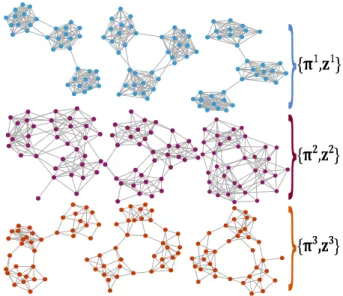
2.1 Objective of strata multilayer stochastic block model (sMLSBM). Each of theL = 9networks here represents a layer in a multilayer network. Ev-ery network layer has N = 36 nodes that are consistent across all layers. There areS = 3strata as indicated by the three rows and the colors of nodes. Clearly, network layers within a stratum exhibit strong similarities in com-munity structure. That is, although each layer follows an SBM withK = 3 communities, the SBM parameters are identical for layers within a strata but differ between layers in different strata. We would like to partition the layers
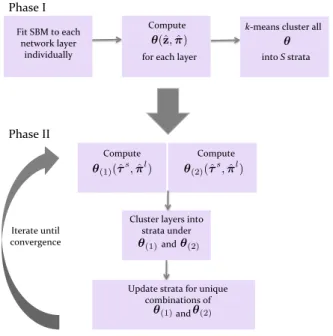
into their appropriate strata and learn their associated SBM parameters,πsandZs. . . 42 2.2 Schematic illustration of our algorithm: Our algorithm for fitting an sMLSBM
is broken up into two phases: an initialization phase to cluster layers into strata, and an iterative phase that allows learning of node-to-community and
layer-to-strata assignments. . . 44
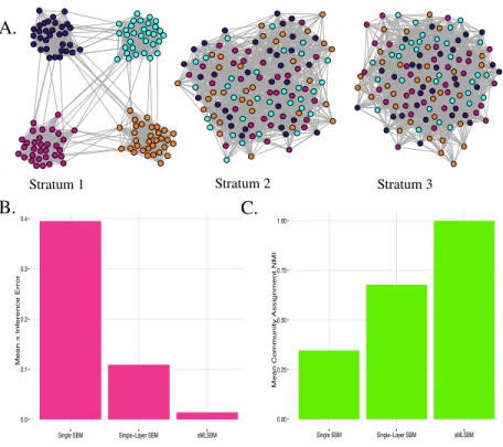
2.3 Synthetic experiment comparing sMLSBM to other SBMs. A. We speci-fied a model withS= 3strata andL= 10layers per stratum. A representative layer from each stratum is plotted. Note that nodes in all networks are colored according to their community membership in stratum 1. Each network has N = 128nodes,K = 4communities and mean degree,c= 20. Theps
in pa-rameters fors= 1,2and 3 are 0.6, 0.4 and 0.25, respectively. Corresponding values ofps
out were selected to maintain the desired expected mean degree, c=20. B. We fit 3 types of models to the 30 network layers: i) single SBM: fitting a single SBM to all of the layers; ii) single-Layer SBM: fitting an indi-vidual SBM to each layer; and iii) sMLSBM: identifying strata and fitting an SBMs for each strata. Each model yields an estimateπslfor the true SBM of
each layerl, which is denotedπl. Heres
ldenotes the inferred strata for layerl. On the vertical axis we plot the mean`2 norm error||vec(πl)−vec(πsl)||2.C.
For each of the three models, we computed the normalized mutual information (NMI) between the true node-to-community assignmentszland the inferred
valueszsl. . . 50
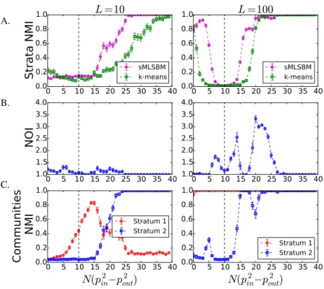
2.4 Synthetic experiment with two strata.We conducted numerical experiments with multilayer networks withN = 128nodes, mean degreec= 16,S = 2 strata andK1 =K2 = 4communities. The networks contained eitherL= 10
(left column) orL= 100layers (right column), which were divided equally into the two strata. For stratum 1, we fixed the quantity N(p1
in −p1out) = 10, which fully specifies (p1
in, p1out) since setting c = 16 also constrains these parameters. In contrast, we vary N(p2
in−p2out). A. As a function of N(p2
in−p2out), we plot the mean NMI to interpret the ability of sMLSBM to recover the true layer-to-strata assignments. We compare the performance of sMLSBM (purple curve) to generick-means clustering (green symbols) of adjacency matrices.B.We plot the mean number of iterations (NOI) required for Phase II of our algorithm to converge.C.Finally, we measure the quality of node-to-community assignment results by plotting the mean NMI between the true node-to-community assignments and those inferred with sMLSBM in
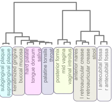
2.5 Comparison of sMLSBM on the OTU interaction networks (Friedman and Alm, 2012) for each of the body sites to a reducibility hierarchy (De Domenico et al., 2015b).As described in the text, we consider a multiplex network withL= 18layers andN = 213nodes, which we group here into S = 6strata, while the dendrogram was generated by the method employed as the precursor to the reducibility framework. Colored boxes around the leaves
of the dendrogram designate the body site to strata assignments obtained with sMLSBM. 56
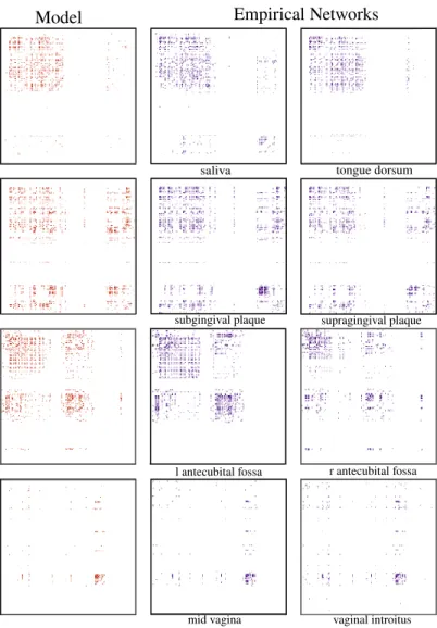
2.6 Visualization of Strata in SparCC Networks. We visualize the adjacency matrices for SparCC networks that encode microbiome interactions at body sites. In each panel, a colored dot at position(i, j)indicates the existence of an edge(i, j)in the corresponding network layer. The four rows correspond to four different strata. In column 1, we show a sample network generated from the SBM parameters,πsandZs, that we inferred for that stratum. In Columns 2 and 3, we show SparCC networks from that particular stratum. Note the
strong similarity across each row. . . 57
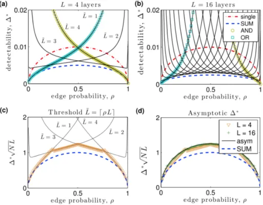
2.7 Layer aggregation enhances the detectability of community structure.Layer aggregation enhances the detectability of community structure. (a),(b). We plot the detectability limit∆∗ versus mean edge probability ρfor a single network layer (red dot-dashed curves), the aggregate network obtained by summation (blue dashed curves), and aggregate networks obtained by thresh-olding this summation at L˜ ∈ {1,2,3,4}(solid curves). Gold circles and cyan squares highlightL˜ = L andL˜ = 1, which we refer to as AND and OR networks, respectively. Results are shown forN = 104 nodes with (a)
L = 4and (b)L = 16layers. (c) ForL = 4, we show∆∗ versusρfor the optimal threshold L˜ = dρLe(orange triangles), which lies on the solution curves forL˜ ∈ {1, . . . , L}(solid curves). (d) We show ∆∗ for L˜ = dρLe
withL ∈ {4,16}. These piecewise-continuous solutions collapse onto the asymptotic solutionδasym∗ (black curve) asLincreases. In panels (c), (d), we
additionally plotδ∗for the summation network (blue dashed curves). . . 64
3.1 Superpixel coarse-graining of an image before segmentation. An image can be represented by a1147×1147grid of pixels (left). Representing the image with 600 super pixels (right), reduces the size of the image and hence
the segmentation problem is to partition the set of 600 super pixels. . . 66
3.2 Defining super nodes. To define the super node representation of a network, we selectSseeds and agglomerate local regions around them to create super nodes. This then leads to a new network with weighted edges between theS
super nodes upon which community detection can be more efficiently applied. . . 71
3.3 Choosing seeds in a synthetic network. The identification of 20 seeds with the CoreHD algorithm in a network generated from a stochastic block model
3.4 Schematic of possible partition comparisons. We outline the types of possi-ble comparisons between partitions generated according to various combina-tions of network representation and community detection method. According to these comparison rules, we compute normalized mutual information (NMI) between all pairs of networks satisfying the comparison criteria. The col-ored circles in the schematic represent a single partition generated under the corresponding network representation and community detection algorithm combination. Circles are colored (in each column) by each of the four possible representation/community detection method combinations. InA-C, we outline the types of comparisons we perform in subsequent figures. A.To compare the usefulness of the super node representation in identifying communities retrieved using the full network, we compare pairs of networks with different representations under the same community detection algorithm. B.Due to the stochastic nature of both the Louvain algorithm and SBM fitting, this comparison seeks to quantify partitions generated under the same network representation and method.C.Finally, we consider pairs of partitions gener-ated under the same network representation and different community detection
algorithms. . . 77
3.5 Super Node Quality. We computed normalized mutual information (A.) and under segmentation error (B.) for networks represented by between 100 and 600 super nodes. Line type and color indicate the community detection algorithm applied (Louvain algorithm or SBM fitting). Each curve indicates the mean across 5 super node representations. The shaded area shows standard deviation.A.Normalized mutual information between the full and super node representations of networks [i.e. NMI(zF ull,zSN)]. A network representation with more super nodes. generally increases the NMI between full network and super node network representations. Horizontal lines indicate the mean pairwise NMI between 10 runs of the Louvain algorithm and SBM result on the full network (pink and gold, respectively). Given the high variability between multiple runs of the same algorithm on the full network, adding more super nodes can only improve the NMI between the full and super node representation to the observed level of similarity observed between algorithm runs. B.The log under segmentation error for super node representations. Defining a super node representation with more super nodes generally decreases the under
segmentation error. . . 78
3.6 Runtimes. We compare community detection runtimes (in seconds) with the Louvain algorithm and by fitting an SBM on the full networks and super node representations for the 9 data sets. (A.)Louvain on the full network. (B.)
Louvain on the super nodes. (C.)SBM on the full network.(D.)SBM on the
3.7 Quantifying partition variability.For each of the 9 networks, we obtained 10 different partitions by the Louvain algorithm and 10 different SBM fits un-der the default (A.) and matched settings (B.). To assess the similarity between partitions within and between a community detection algorithm in networks under the the super node representation, we computed pairwise normalized mutual information (NMI) as a function of the number of super nodes. The pink and blue curves show the mean pairwise normalized mutual information between all pairs of 10 partitions under Louvain and SBM fitting, respec-tively. The gold curves compare pairs of partitions under different methods. Shaded area denotes standard deviation. Horizontal lines indicates the mean pairwise NMI between partitions under the full network representation for within Louvain and SBM partition comparison (pink and blue, respectively) and between Louvain and SBM partition comparison (gold). Overall, the super node representation is useful for reducing the disparity between the partitions
obtained under different methods. . . 81
3.8 Agreement of community assignments with local connectivity. We study how consistent partitions are within local neighborhood regions of the network by examining how well a node’s neighbors (for various order neighborhoods) can be used to predict its community assignment, under some community partitionz. For each community in a partition, we give a binary prediction of whether a node is assigned to that community, based on probabilities we compute for a node from its neighbors. Sweeping the parameterpthat sets the probability required for a node to be assigned to a community, we compute ROC curves for each community and report the minimum AUC value observed. PanelsA-Dshow minimum AUC values observed as a function of neighbor-hood order for communities obtained from the full networks and super node representations by Louvain and by SBM. Line color indicates network and line type indicates communities obtained from the matched and default parameters used by the algorithms on the full networks. PanelsE-Hvisualize the com-munities obtained in the As22 data on the full network (default parameters) and super node representation (SN) under Louvain and SBM, with node colors
indicating community memberships. . . 82
4.1 Modeling community membership in terms of attributes and connectivity. Node-to-community assignments specified byZare determined in terms of adjacency matrix information,Aand attribute matrix information,X.Aand Xare assumed by be generated from a stochastic block model and a mixture
4.2 Synthetic Example. We generated a synthetic network withN = 200nodes, K = 4communities and an 8-dimensional multivariate Gaussian for each community. A. A visualization of the adjacency matrix for this network where a black dot indicates an edge. We observe that there is an assorta-tive block structure (blocks on the diagonal), but there are also many edges between communities making the true community structure using only con-nectivity harder to detect. B. We performed PCA on the N ×p attribute array and plotted each of the N nodes in two dimensions. Points are col-ored by their true community assignments,z. Clustering the nodes according to only connectivity, only attributes, and with the attributed SBM, we quan-tified the partition accuracy with normalized mutual information, yielding
NMI(z,{zconnectivity,zattributes,zattribute sbm}) ={0.65,0.68,0.83}. . . 92
4.3 Detectability Analysis in Synthetic Example. To understand how attribute information can be combined with connectivity to assign nodes to communities accurately, we generated synthetic networks for within-probabilities ofpin between 0.05 and 0.3 with correspondingpoutor between-community prob-abilities such that the mean degree of the network was 20. For each of these synthetic networks, we used the attributes from the analysis in figure 2 to fit the attributed SBM. Here, we plot the correctness of the node-to-community assignment with normalized mutual information using the partition obtained from regular SBM (blue) and the partition under the attributed SBM model fit (pink). For each combination ofpinandpout, we generated 10 networks and hence the bands around the points denote standard deviation. Incorporating attributes with the attributes stochastic block model improves results, partic-ularly near and below the detectability limit, and appears to smooth out the
sharp phase transition. . . 94
4.4 Microbiome subject similarity network: A visualization of the 121 node microbiome subject similarity network with nodes colored by the partition using the classic (A.) and attributed (B.) stochastic block model. A.Fitting the classic stochastic block model to the network, 7 communities were identi-fied.B.Fitting the attributed stochastic block model to the network with the attributes being the first 5 principle components of each subject’s OTU count vector (metagenomic profile), 6 communities were identified. Incorporating attributes in inferring this partition removed some of the noise in the partition
on the network, specifically in the mixed purple community in the left ofA.. . . 99
4.5 Link Prediction on the microbiome subject similarity network: The re-sults for link prediction on the microbiome subject similarity network for the attributed SBM, Jaccard, Adamic-Adar and preferential attachment methods. The corresponding AUC values for these methods, respectively are, 0.71, 0.69,
4.6 Collaborative Filtering Accuracy in Microbiome Subject Similarity Net-work: For each of the 121 nodes, we fit a model to the remaining 120 node network and given the node’s closest neighbors (based on network connectiv-ity) sought to predict its 5-dimensional attribute vector. The reported error is the relative errorEbetween the difference between the true attribute vector (xi) and its predicted attribute vector (ˆxi). The mean error inxiis 0.21, as opposed to the neighbor average and weighted neighbor averages, having errors of 0.26
and 0.27, respectively. . . 101
4.7 Protein interaction network. We visualize the 82 node protein interaction network under the classic stochastic block modelA.and the attributed stochas-tic block modelB.In both networks, nodes are colored by their community assignment and the node shape indicates whether the modification status in-creased (square) or dein-creased.A.Nodes colored according to the community partition under the stochastic block model. Nodes are assigned to one of five communities.B.Nodes are colored to the community partition under one of
nine communities. . . 102
4.8 Community entropies in the protein interaction network. We studied the entropy of the 2 class and 6 class classifications of the nodes in A.andB., respectively under the classic SBM (black) and attributed SBM (purple) parti-tions. ForA.−B.the horizontal axis denotes the community index for the particular partition. Nodes belonged to 1 of 5 communities under the classic SBM and belong to 1 of 9 communities with the attributed SBM. Incorporating attributes under both classifications succeeds in breaking up a high entropy community (5) from the classic SBM partition to lower entropy communities
in the attributed SBM partition. . . 103
4.9 Link Prediction in the protein interaction network. Performing link pre-diction using the attributed SBM, Jaccard, Adamic Adar, and preferential attachment. The corresponding AUC curves for these methods were 0.61, 0.58,
0.58, and 0.51, respectively. . . 104
4.10 Collaborative filtering in the protein interaction network. For each of the 82 nodes, we fit a model to the remaining 81 node network and given the node’s closest neighbors (based on network connectivity) sought to predict its 6-dimensional attribute vector. The reported error is the relative errorE between the difference between the true attribute vector (xi) and its predicted attribute vector (xi). The mean error inˆ xiusing the attributed SBM is 0.21, as
5.1 Overview of the method. Our test first labels the nodes according to attribute information,˜z. Then in a collection ofT trials, a sample oflnodes is treated as labeled, according to˜z. In each trial, a label propagation task is performed to predict the probability distribution over communities for the unlabeledN−l nodes. The entropy of the node-to-community assignment probabilities is used as an estimate of how well the attributes align with connectivity. Also in each trial, ˜zis permuted and subjected to the label propagation task to compute a ‘null’ entropy value. After repeating this process inT trials, the empirical p-value is calculated based on the overlap between the null entropy distribution
and the empirical entropy distribution. . . 110
5.2 Properties of the empirical p-value. To understand the properties of our empiricalp-value, we generated a synthetic network,Afrom an SBM with N = 200nodes,K= 4communities. The vector of continuous attributes for a nodei, (Xi) was drawn from a multivariate Gaussian distribution parameter-ized by its community assignment (zi) or{µzi,Σzi}. In these experiments, we
permuted varying fractions of˜zand observed the effects on entropy and em-piricalp-value.A. We used tSNE to visualize the two dimensional projection of the 200 nodes. For the most part, members of the same community cluster together.B.We plotted the empiricalp-value as a function of the proportion of labels permuted and observed decreased statistical significance (increased empiricalp-value) with an increasing proportion of permuted labels. C.We plotted the empiricalp-value as a function of the mean entropy (E) across T = 1000trials used to generate the entropy distributions for each experiment. Increased entropy corresponding to a larger proportion of˜zpermuted leads to
a decreasedp-value. . . 114 5.3 Comparison with BESTest. We sought to understand the relationship
be-tween our empiricalp-value and that computed according to BESTest. To study this, we used the same experiment described in Figure 5.2, where we varied the proportion of permuted labels from˜z. We denote our empirical p-value by ‘LP empiricalp-value. A.We plotted the BESTest empiricalp -value against our LP empiricalp-value.B.We plotted the BESTest empirical p-value as a function of the BESTest entropy. BESTest gives a significant empiricalp-value for a much wider range of entropy levels than our test. C.
The experiments produced a wide range of entropies under BESTest, which are captured by corresponding differences in our empiricalp-value. D.We compared the BESTest approach to computing entropy to our LP method and
5.4 Analysis of the strength of structural communities.To understand the effect of network structure on our test, we generated synthetic networks from stochas-tic block models with various pin (within-community) and pout (between-community) parameters. Networks were generated withpinvarying between 0.05 and 0.45 and we chose a correspondingpoutsuch that the mean degree was 30. We usedpin/pout as a proxy for the strength of community, with a higher value of this ratio indicating a stronger community structure with more within-community edges and fewer between community edges. For each pin,poutcombination, we generated 10 synthetic network realizations.A.We plotted the relationship between our LP entropy andpin/pout. The shaded area denotes standard deviation of the mean entropy over the 10 networks for eachpin,poutcombination. B.Similar to (A.), we plotted the mean empirical p-value over theT = 1000trials used to generate the entropy distributions,E andEperm. For largepin/pout, the empiricalp-value became more significant. The shaded area denotes standard deviation of empiricalp-value over the 10 networks for eachpin,poutcombination.C.Finally, we plotted the relationship between the mean entropy over theT=1000 trials,Eand the empiricalp-value.
These values are strongly correlated withr= 0.91. . . 117 5.5 Alignment of markers with communities.We considered each of the
possi-ble 51 features in the single cell data and their potential to be used as markers of particular inferred cellular phenotypes. We identified 10 communities (or inferred phenotypes) under the Louvain algorithm, producing a partition of the network,z. We then created a partition,˜zfrom each attribute in isolation. For each attribute and its induced partition of the nodes,˜z, normalized mutual information (NMI) was used to measure the discriminative power of the marker in distinguishing network communities, or NMI(˜z,z). We expected that our p-value should align with this NMI measure in that markers leading to high NMI between the induced˜zandzshould have more significantp-values.A.
We used a histogram to visualize the distribution of NMI values across the 51 possible markers, with many of them leading to low NMI (between 0 and 0.1). B.Similar to (A.), we visualized the empiricalp-value for the 51 possible markers. C. We compared the relationship between the empiricalp-value (vertical axis) and NMI(˜z,z) (horizontal axis) across the 51 possible markers. As expected, we observed these quantities to be anti-correlated in that more
5.6 Validation with well and poorly aligned markers. We used two markers with different correlation strength with communities as another validation of the computed entropy under label propagations. First, we defined a labeling of the nodes,˜zbased on marker (Rh103)Di<BC103>that did not vary across communities in its expression, and hence not discriminate between the commu-nities.A.We visualized the distribution ofE(purple), in comparison toEperm
(gold). Since this marker has low discriminative power, we expected the shown overlap betweenEandEperm. B.We plotted the network of the 1000 single cells and colored nodes by their expression of (Rh103)Di<BC103 >, with lighter colors indicating higher expression. It is difficult to notice clustering in this network between cells with similar expression values. C.Conversely to the result shown in (A.), we chose a marker with high discriminative power, (Nd146)Di<CD8>. Again, we show the distribution ofE(purple), in com-parison toEperm(gold). Since this marker has good discriminative power,E andEpermdo not overlap.D.We plotted the network of single cells, with nodes
colored according to the intensity of (Nd146)Di<CD8>, with lighter colors
indicating higher expression. . . 120
5.7 Variation of markers with significant empiricalp-values across commu-nities. We computed the empirical p-values induced by the partition˜z for each of the 51 markers and looked closely at the top and bottom 5 markers, as inferred through the empiricalp-value. Since a quality marker in this case is said to be one that induces a labeled of the nodes,˜zsimilar to the result obtained underz, we expect the expression of such a marker to vary across communities. In this plot, we show the expression of each marker as a function of the community index. The family of orange-colored lines correspond to the top 5 predicted markers (according to empiricalp-value). From all of these lines, the expression varies across communities. Conversely, we plotted the lowest-ranked markers (in terms of empiricalp-value and their expression is
relatively constant across all communities. . . 121
6.1 Microbial co-occurence networks for each patient cohort. We constructed networks with SparCC in the ALI and non-ALI cohort networks (left and right, respectively). Four communities were identified in each network. Nodes are
colored by their community assignment. . . 126
6.2 Predictive functions for community classification. We used a set of 328 filtered functions to predict OTU-to-community assignment in the ALI and No ALI networks. Here we show show the functions identified as the most strong predictors for each community in the ALI and No ALI networks (left and right, respectively). Functions with more discriminative ability in classification from
LIST OF ABBREVIATIONS & COMMON NOTATION
SBM Stochastic Block Model EM Expectation Maximization
sMLSBM Strata Multilayer Stochastic Block Model MLSBM Multilayer Stochastic Block Model A Network adjacency Matrix
SN Super Node
z For a network withN nodes, this is the lengthN vector of node-to-community assignments zi The community assignment of nodei
Z The indicator matrix of node-to-community assignments zik A binary indicator of whether nodeibelongs to communityk. ALI Acute lung injury
OTU Operational taxonomic unit DAG Directed acyclic graph MCMC Markov Chain Monte Carlo
pin Within-community edge probability under stochastic block model pout Between-community edge probability under stochastic block model
CHAPTER 1 Introduction
Network data appears widely across fields as a data structure for modeling relational information between a set of entities. In recent years, networks have become an indispensable data mining tool, as they allow for tasks such as data visualization (Traud et al., 2009), clustering (Fortunato and Hric, 2016), and prediction tasks (Wang et al., 2014; Deng et al., 2014). Motivated by problems in fields such as, biology (Larremore et al., 2013), medicine (Aghaeepour et al., 2017), neuroscience (Bassett et al., 2011), and social science (Greene and Cunningham, 2013), the field of network analysis has gained popularity and seeks to develop tools for understanding the associated network data. The main objectives in creating tools for the analysis of network data is to enable effective modeling, prediction, and data interpretation. In this thesis, we present three new methods that enable a more thorough understanding of the structural organization patterns in networks throughcommunity detection. The objective of community detection is to partition the network nodes intocommunities, such that members of a community have similar connectivity patterns. With an increasing amount of more challenging types of network data, such as those containing multiple relational definitions between a set of nodes, standard community detection approaches are often insufficient. In this thesis, we will look in depth at how to handle communities in networks that aremultilayer, large, and attributed. We then present several case studies in each of the developed methods in applications such as, microbiome analysis, protein interaction network understanding, and mining in social networks. We show that the successful identification of communities in these types of networks allows the network to be used for tasks such as, efficient summarization, prediction, and classification.
prioritizing further experiments. Finally, we discuss challenges in the field of community detection and how this work addresses some of these problems.
1.1 Network Notation and Basic Summarization
In this section, we provide some basic notation and summarization techniques for representing and summarizing networks.
1.1.1 Representing relational information
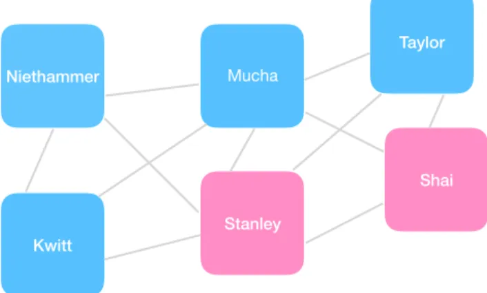
Humans frequently benefit from network applications for tasks such as, viewing relevant queries from a google search, enjoying a suggested movie on Netflix, or interacting on a social network platform. The basic building blocks of networks are nodes, representing entities in a systems, and edges, encoding connections their physical or inferred connection or similarity. Figure 1.1 shows a collaboration network between the six people that made the work in this thesis possible. An edge between a pair of people indicates if they have written a paper together.
Mucha
Stanley Niethammer
Kwitt
Shai Taylor
Figure 1.1:A simple network example (coauthorship).A co-authorship network with an edge between a pair of people if they have written a paper together.
aij = 1 if nodeiand nodejare connected aij = 0 otherwise.
In theweightedcase of undirected networks, edge weights are some real number and are frequently quantities such as correlation or pairwise similarity. A simple extension ofAto an undirected, weighted network wherewis the edge weight between nodesiandj, computes the adjacency matrix entryaij as,
aij =w if nodeiand nodejare connectedwith weightw aij = 0 otherwise.
Alternatively, the assumption of a symmetric relationship between a pair of nodes that node i connects to nodej and nodej connects to node imay be unrealistic. For example, on some social network platforms, userican follow userj, but userjdoes not necessarily need to follow useri. This type of network is known as adirectednetwork. While directed networks are frequently discussed in the network science literature, we will not introduce them here because they are not directly involved in any work in this thesis.
1.1.2 Network Summary Statistics
Figure 1.2:Hairball network.Networks are often noisy data structures and lack an immediate straight forward structural interpretation.Image fromhttps://cs.umd.edu.
1.1.2.1 Example: A network representation of single cell data and simple summary statistics
An initially overwhelming network structure can be mediated by tools to break down, quantify, and characterize structural patterns. In this section, we will describe a few of the essential summary statistics and analyses that can be performed and will be seen throughout this thesis.
To illustrate these quantities in an applied context, we will compute them on an example network shown in Figure 1.3. This network is constructed from a single cell mass cytometry dataset, which was originally described in Ref. (Wong et al., 2015) and released publicly and processed using the Cytofkit R package (Chen et al., 2016). Each node represents a single cell and is represented with 52 features for a mass cytometry analysis. Briefly, mass cytometry is a technique to simultaneously measure multiple immunological features in a cell or tissue (Bendall et al., 2012). From this data matrix, we created a network by selecting 500 cells and building ak-nearest neighbor network withk= 5. This means that for a nodei, we found its5nearest neighbors according to Euclidean distance, and connected them all to nodei.
1.1.2.2 Degree Distribution
Figure 1.3:Network of single cells. We constructed a network from mass cytometry profiling among 500 cells in single cell dataset. Each cell has 52 measured immune features. In this network, each node is a single cell and is connected to its 5 nearest neighbors.
degree(i) =X j
aij (1.1)
1 2 5 10 20
0.01
0.05
0.50
5.00
Degree
C
umu
la
tive
F
re
qu
en
cy
Degree
F
eq
ue
ncy
5 10 15 20
0
50
100
150
200
250
A.
B.
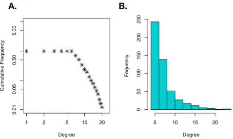
Figure 1.4:Degree distribution for the single cell network.We visualize the degree distribution in the single cell network presented in Figure 1.3.A.We compute a cumulative distribution plot for degree.B.
Node degrees can also be visualized with a simple histogram.
1.1.2.3 Centrality
To compute the importance of a node in the network it is common to compute a centrality score. There are many definitions of centrality, and we will only present a small subset of these definitions here. We benefit from the idea of high centrality nodes when we do a Google search and have a relevant page of returned search results. In this section, we introduce degree centrality, betweenness centrality, and eigenvector centrality. Given that each of these measures is computed differently, each is intended to capture a different structural aspect of the network.
Degree centrality
Degree centrality is the most simple centrality measure because it is just simply a node’s degree. This means that under this measure, the most important nodes in the network are nodes with high degree. This centrality is attractive because it is easy to compute, having complexity in a sparse network ofO(E) (whereEis the number of edges). We define degree centrality of nodei,D(i)as,
D(i) =X j
aij (1.2)
Betweenness centrality
Degree Betweenness Eigenvector
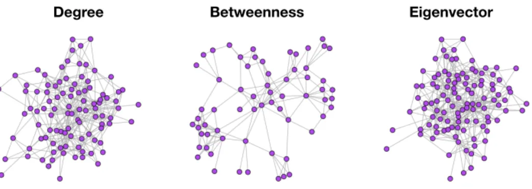
Figure 1.5: Centralities on the single cell network. The second order ego network for the highest centrality nodes in the single cell network according to degree, betweenness, and eigenvector in the left, center, and right plots, respectively. These plots are meant to emphasize how each of these centrality measures prioritizes different kind of structure.
So, if a node appears on many of the shortest paths between node pairs, then it is considered to be an important node. We define betweenness centrality for a nodei,B(i)as
B(i) = X i6=j6=t
σjt(i) σjt
, (1.3)
whereσjtis the total number of shortest paths between a pair of nodes,jandt. Similarly,σjt(i)are all of the shortest paths betweenjandtthat pass throughi.
Eigenvector centrality
The idea behind eigenvector centrality is that a node should be prioritized not only based on its degree, but the degree of its neighboring nodes. That is, a node connected to other ‘important’ or high degree nodes should be ranked higher than one connected to many low degree nodes. 1 The eigenvector centrality for nodei, can be computed using the spectra of the adjacency matrix,A. In particular, the vector of centralities,xis the one satisfying the eigenvector equation,
Ax=λx. (1.4)
Because centralities are non-zero, the solution must be an eigenvector with all positive entries. Since multiple eigenvalues (λ) correspond to non-zero eigenvectors, the eigenvector corresponding to the largest
eigenvector is used and the centrality scores for each node reflect its relative importance in comparison to the rest of the nodes.2 Moreover, thei-th entry ofxgives the eigenvector centrality for nodei.
We visualized the results of each of these three presented centralities on the single cell network data in Figure 1.5. Under each of the centrality measures, we selected the the highest-ranked centrality node and focused on its local ego network. This is shown for degree, betweenness, and eigenvector centralities in the left, middle, and right panels respectively. In particular from these high centrality nodes, we visualized their corresponding order 2 ego networks. The ego network for nodeiis simply the subgraph of all nodes within two hops of nodei. This visualization gives a sense of what kinds of connectivity patterns each centrality measure favors. For example, we see that degree and eigenvector centrality have similar ego networks, as they are capturing nodes with a lot of connections. However, the ego network of the high betweenness centrality node is serving as more as a bridge between densely connected parts of the network.
1.2 Introduction to community detection
While centrality measures allow for the prioritization of individual nodes in the network, it is also useful to look at sets of similar nodes in terms of how they are situated in the network. Each of these sets of similar nodes is known as acommunity. A community in a network is broadly defined as a set of nodes of who share something in common in terms of their connectivity patterns in the network. One can think of a community as a clustering problem on networks, where the objective is to define sets of nodes that maximize the within-community node similarity. The most basic type of community to understand is a network with assortative community structure. In this case, nodes are tightly connected to each other but more sparsely connected to the rest of the network. An example of a network with assortative community structure is shown in Figure 1.6. Communities in the network are outlined with pink dotted lines.
Alternatively, networks can have a disassortative structure where the between community edge density exceeds the within-community density. Finally, a core periphery structure can arise when there is a central core in the network that connects to the rest of the network and a set of peripheral nodes that connect to the core, but not to each other. Similar to how the shape or distribution of a set of points in
2
severity 6444
Figure 1.6:Assortative Community Structure.This network is an example of assortative community structure, where nodes are tightly connected to each other and more sparsely connected to the rest of the network. Each community is outlined with a pink dotted line.
high dimensional space informs the ideal clustering algorithm to use, aspects of these diverse types of community structure often prescribe which algorithm to use. For a great explanation about common types of community structure in network data which patterns have been observed in the human brain, please refer to Betzelet al.(Betzel et al., 2018).
In this section, we have only briefly introduced the history and intuition behind community detection. Since it is a well-developed domain of network science, the interested reader can refer to one of the comprehensive review articles (Lancichinetti and Fortunato, 2009; Fortunato and Hric, 2016; Shai et al., 2017; Mucha et al., 2010a)
1.3 Community detection methods
modularity maximization, as those are the the approaches considered throughout the novel work in this thesis.
1.3.1 Notation for Community Detection
We first define some common notation for community detection. For a network withN nodes, we use a community detection algorithm to separate these nodes intoKcommunities. To encode the node-to-community assignments, we use the lengthN vector,z, wherezi gives the community assignment for nodei. For some applications, we also specify theN ×K matrix,Z, which is a binary indicator matrix, wherezikindicated whether nodeiis assigned to communityk. These two pieces of notation will be used across each of the described algorithms.
1.3.2 Quality function maximization with modularity
In quality function optimization approaches one first specifies an objective function in terms of a partition of the nodes. The most common quality function for this task is known as modularity (Newman, 2006a). Modularity first defines a null model for community structure where edges are placed between groups randomly. With this as the starting point, the partition that optimizes modularity is the one that is maximally different from this null model. In particular, this null model is a random graph model, known as the configuration model (Bender and Canfield, 1978). To generate anN-node network from the configuration model, one first specifies a fixed degree sequence,D={ki, k2, . . . , kN}. From this sequence, nodes are connected withkistubs that will ultimately be connected together. Finally, the graph is constructed by randomly choosing pairs of the created stubs and joining them. Based on how this network was generated, it is easy to specify the probability that an edge exists between a pair of nodes,i andj, orP(aij = 1)as
P(aij = 1) = kikj
2M. (1.5)
Here,kiandkj represent the degree for nodesiandj, respectively, andM is the total number of edges in the network.
Q= 1 2M
X i,j
aij −γ
kikj 2M
δ(zi, zj) (1.6)
Here,γ is a resolution parameter (Reichardt and Bornholdt, 2006) that controls the scale of com-munity size. Large values ofγ favor more small communities while smaller values enforce fewer large communities.
In order to determine z, the most computationally efficient approach is known as the Louvain algorithm (Blondel et al., 2008). The Louvain algorithm is an agglomerative heuristic, which initially starts with each node in its own community and in the first pass moves single nodes into the same group if their merge leads to an increase in modularity. Each group of nodes assembled after this first pass becomes a new node in the network and a new weighted network is created between the set of new nodes. The weight on the edges of the new network are the number of edges from the original network that go between the sets of merged nodes. This process is continued iteratively until the modularity no longer increases. The reason that this approach is so computationally tractable is because the gain in modularity, ∆Qof merging two groups of nodes can be explicitly computed in closed form.
Modularity has shown to be effective in applications from neuroscience (Meunier et al., 2009) to image segmentation (Browet et al., 2011). It has also shown to be effective in clustering high dimensional data that has been used to create a network. In Figure 1.7, we used tSNE (Maaten and Hinton, 2008) to project the 52-dimensional single cell data into 2 dimensions. Points are colored by their cluster assignment according tok-means. We first performedk-means on the original 51 dimensional data (left) and Louvain community detection on the 5 nearest neighbor network representation (right). One benefit of the Louvain algorithm is that it does not require specifying the number of clusters. Moreover, in this example, the Louvain algorithm maximized modularity by partitioning the network into 10 clusters. To compare the results under the same number of clusters, we also clustered the original data into 10 clusters. From these two partitions, we observe that creating a network representation of the data before clustering assists in identifying the smaller, less prominent clusters.
1.3.3 Identifying communities with probabilistic approaches
−15 −5 0 5 10
−
20
−
10
0
10
20
kmeans
tSNE 1
tSNE 2
−15 −5 0 5 10
−
20
−
10
0
10
20
Louvain
tSNE 1
tSNE 2
Figure 1.7: A comparison of k-means and the Louvain algorithm on the single cell network. A comparison of the results of clustering results on the the single cell dataset throughk-means on the original 52-dimensional data (left) and by the Louvain algorithm on the nearest neighbor network (right). Each of the single cells (or nodes in the nearest neighbor network) is visualized by a 2-dimensional projection frin tSNE. Points are colored by their cluster membership underk-means on the original data (left) and Louvain community detection (right). Applying community detection to the nearest neighbor network seems to smooth out the partition and identify some smaller clusters.
the inferred community assignments. For example, given nodesiandj, one may modelP(aij = 1) as g(zi, zj), where g(·) is some rule based on the node-to-community assignments. Two common probabilistic community detection models are the stochastic block model (Snijders and Nowicki, 1997a) and the affiliation model (Yang and Leskovec, 2012). The definition and description of these models and inference techniques are described in depth in this section. To facilitate working with probabilistic models, we first introduce some notation and background on inference techniques.
1.3.3.1 Probabilistic graphical models for statistical inference
Probabilistic community detection methods are one approach to community detection that seek to model edge existence based on the inferred node-to-community assignments. In doing so, the objective is to learn the node-to-community assignments that make the structure of the observed network the most likely. This is accomplished through likelihood optimization. To fit a probabilistic network model to data, we will define some useful notation and concepts that help simplify writing down and interpreting the likelihood.
node-to-Figure 1.8:Directed Acyclic Graph.A directed acyclic graph (DAG) is formed based on dependency between random variable and allows for a fully factorized probability distribution. Nodes represent random variables and a directed edge from nodeito nodejindicates that nodejdepends on nodei.
community assignments, andA, the observed adjacency matrix. Probabilistic graphical models (Koller and Friedman, 2009) enable efficient specification and manipulation of large probability distributions through semantic structures.
As a brief example, given a set of random variables,{A, B, C, D, E, F}, we seek to compute the joint distribution,P(A, B, C, D, E, F). This joint distribution can be expressed with a directed acyclic graph (DAG), whose structure encodes dependencies between random variables. The DAG allows for the representation of the joint distribution in a factorized way, which is computationally useful. A DAG between the set of random variables, {A, B, C, D, E, F}is shown in Figure 1.8. Each node in the graphical model represents an random variable and a directed edge from nodeito nodejimplies that nodejdepends on nodei.
To translate a DAG between a set ofN random variables,X = {X1, X2, . . . , XN} (also in this context referred to as a Bayesian network) to its joint distribution, we rely on the chain rule for Bayesian networks (Koller and Friedman, 2009), which specifies that a DAG factors according to its parent/child relationships with,
P(X) = Y i=1:N
P(Xi |Xπi). (1.7)
P(A, B, C, D, E, F) =P(A)P(B |A)P(C|B)
×P(D|B, G)P(E |D, B, C)P(F |E).
(1.8)
This introduced idea will help in subsequent sections to express a model graphically, write down the model likelihood, and use the likelihood to optimize for the most appropriate model parameters.
1.3.3.2 Stochastic Block Model
In this section, we introduce the most popular probabilistic model for community structure, known as the Stochastic Block Model (Snijders and Nowicki, 1997b). This model is popular and has been studied extensively, due to its simplicity and intuitive interpretation. The crucial assumption of the stochastic block model is that nodes within a community are connected to nodes within their community and to other communities in a characteristic way. For an undirected, unweighted network with adjacency matrixA, we seek to partition each of theN nodes into one ofKcommunities. We denote the node-to-community assignments asz, withzispecifying the community assignment of nodei. Here,zis a latent variable, with each entry taking on 1 ofKstates (community labels). Figure 1.9 shows the dependency relationship between the node-to-community assignments (z) and the network’s adjacency matrix (A). Here, the
node-to-community assignments are treated as latent variables because we seek to identify thezthat makes the observed adjacency matrix,A, the most likely. To model the objective that members within and between communities connect in characteristic ways, the model fitting procedure requires learning a set of within and between community connection probabilities. Under this approach, edges are treated as independent and identically distributed and deciding whether or node an edge exists between a pair of nodes is the learned connection probability between the communities to which each of the nodes belong.
Using the factorization rules described in section 1.3.3.1, we can specify the complete data log likelihood betweenzandAas,
Z
A
Figure 1.9:SBM Graphical Model.A graphical model is used to model the dependency between the node-to-community assignments,zand the observed network adjacency matrix,A.
To further specify these communities, we will define additional notation. First, letπK×K ={πij} be the matrix that specifies the within and between community edge probabilities. Using this information, we can model the probability of an edge existing between nodesiandjas,
P(aij = 1)∼Bernoulli(πzi,zj). (1.10)
Here,πzi,zj is the connection probability between the inferred community assignments of nodesi
andj.
Further, we letZi ={Zi1, Zi2, . . . Zik}be a collection of binary indicators whereZik is 1 if node ibelongs to communitykand 0 otherwise, We also letαk be the probability that a node belongs to communityk. With all of this information, we can write down each term of the complete data likelihood.
First,
log(P(Z)) =X i
X k
Ziklog(αk). (1.11)
Next,
log(P(A,Z)) =X i6=j
X k<l
ZikZil[aijlog(πkl) + (1−aij) log(1−πkl)] (1.12)
P(z|A). To optimize the lower bound ofL(A), we seek theRAthat is as close as possible toP(z|A). In other words, we define the lower bound ofL(A)asT(RA), with
T(RA) = logL(A)−KL[RA(z),P(z|A)]. (1.13)
Here KL denotes the Kullback-Leibler divergence (KL divergence) and the best approximation will be the value that makes the KL divergence the smallest. Jaakkolaet al.present a mean field approximation for the posterior distribution (Jaakkola, 2001) as,
RA(z) =Y i
h(Zi;τi). (1.14)
Here τ = (τi1, . . . , τiK) and τik is the approximation that node i belongs to community k, or P(Zik = 1|A). Furthermore,h(·;τi)denotes the multinomial distribution with parameterτ.
Daudinet al.(Daudin et al., 2008) show that the optimal estimate forτikdenotedτˆiksatisfies
ˆ τik∝αk
Y j6=i
Y l
[πaij
zi,zj(1−πzi,zj)
1−aij]ˆτik. (1.15)
Here,αkdenotes the probability that a node belongs to communityk. Furthermore, after computing the set of variational parameters, the updates forα andπ that maximizeT(RA)are also shown by Daudinet al.,(Daudin et al., 2008) to be,
ˆ αk =
1 n
X i
ˆ
τik θql = X
i6=j ˆ
τiqˆτjlaij/ X i6=j
ˆ
τiqτˆjl (1.16)
This formulation of the problem and parameter optimization procedure works well and converges quickly for networks that have assortative community structures and a homogenous degree distribution. We will now explore how this classic formulation of the SBM can be modified to enable a broader application for a variety of networks.
1.3.3.3 Variants to the Classic Stochastic Block Model
The introduced stochastic block model is the most vanilla version in that it makes the assumption that the network is unweighted and that each node is assigned to only one community. The introduced model also does not account for issues that may arise from degree heterogeneity (i.e. a wide degree distribution). Here, we will briefly discuss the approaches that adapt the stochastic block model to handle these issues and assumptions.
Edge Weights
The majority of the stochastic block model literature considers unweighted networks simply because describing a probabilistic model to handle both edge existence and edge weight is a challenging task. In the classic stochastic block model, we are simply modeling whether an edge exists based on the inferred community memberships of the edge stubs. Since edge weights can come in a variety of forms (real-valued, count, etc.), it is difficult to immediately decide what distribution the edge weights should follow. In the past few years, this issue has been tackled in two papers (Aicher et al., 2014; Peixoto, 2018).
First, Aicheret al. developed a model and associated inference technique as the initial efforts toward a weighted stochastic block model. Here, edge weights can be modeled by any exponential family probability distribution. The authors use a mixing parameter that allows for the control of the use of edge existence versus edge weights when learning node-to-community assignments. This method requires an estimate for the number of expected communities,K. However, the paper provides an approach to use Bayes’ factors between two competing values ofKto determine which model is a better fit. The inference for fitting this model is performed through a variational Bayes approach (Attias, 2000).
Degree Heterogeneity
Based on the variety of network structures and types, the assumption that the classic stochastic block model is an appropriate model for even classic unweighted data is often invalid. That is, for some networks, the fitted model may not actually be a good fit, in that samples from the learned model are substantially different from the network. Work by Karreret al.(Karrer and , 2011) introduced a simple extension to the classic stochastic block model, known as the degree corrected stochastic block model. This model is informed by degree distribution as a proxy for the network structure. In networks where there is a wide degree distribution (i.e. many high degree nodes and many low degree nodes), stochastic block model inference tends to partition the nodes into communities of high degree and low degree nodes. The approach for adapting the SBM to this setting is to slightly modify the learnedK×Kmatrix,π
slightly. Here,πij described the number of edges between communitiesiandj. Further, these edges counts are modeled as Poisson random variables. The likelihood of the observed network under this Poisson assumption takes into each node’s degree.
The restriction of single community membership
As it is often observed in social networks, the assumption that every node belongs to only a single community is restrictive. To address this issue, approaches have been developed to allow nodes to participate in a mixture of communities (Airoldi et al., 2008) or be members of overlapping communities (Latouche et al., 2011). Airoldiet al., pioneered the development of the mixed membership stochastic block model (Airoldi et al., 2008), where instead of modeling a node’s membership in each community in a binary manner, the authors allow a node to belong to multiple communities. The generative process for this approach for modeling the existence of an edge between nodespandqin a network withKpossible communities and theK×Kmatrix,θ, representing the between community connection probabilities.
• For each nodep, draw a mixed membership vectorπp∼Dirichelet(α)
• Then for each pair of nodes(p, q), drawzp→q∼Multinomial(πp),zq→p∼Multinomial(πq)
• Sample the edge betweenpandqas,Apq, whereApq∼Bernoulli(zTq→pθzq→p)
memberships of nodespandq towards other nodes in the network are ignored. Moreover, this model adapts the mixed membership stochastic block model to incorporate a higher order resolution of structure by considering each node in the context of its neighbors.
1.3.3.4 Affiliation model and inference
We have previously discussed extensions of the stochastic block model that account for the assump-tion that nodes can belong to multiple communities. Another interesting idea is the idea ofpluralistic homophily, where the probability that two individuals are connected is related to the affiliations of the nodes (Feld, 1981). In other words, the more groups a pair of nodes share, the more likely they are to have a connection. For example, if two people were graduate students studying computational biology at the same university, they are more likely to be connected than a pair of graduate students studying different subjects at the same university. A state-of-the-art method called BIGCLAM was presented for this task by Yanget al. in 2013 (Yang and Leskovec, 2013). The objective here is to model the connection probability between a pair of nodes based on the similarity in their learned affiliations towards communities. To do this, individual nodes are connected with communities with some number of links, with more links from a node to a community indicating that the node has a higher ‘affilation’ to that group. For a network withN nodes andccommunities, the affiliation between nodes and communities is encoded by a matrix,F, whereFucis the learned count of links (again encoding the affiliation), between nodeiand communityc. Similarly, letFuandFv be the community affiliations for nodesuandv. Then the probability that an edge exists between nodesuandv, orP(Auv= 1)is modeled as,
P(Auv= 1) = 1−exp(−FuFvT). (1.17)
The node to community affiliations can be used as a proxy for the total amount of interaction between a pair of nodesuandvwith a Poisson distribution. This modeling paradigm will allow for the straightforward modeling of the probability that an edge exists between the node pair. To do this, the total amount of interaction between nodesuandvis modeled as,
Xuv = X
c Xc