Meijer_unc_0153D_18767.pdf

PRECISION MODELING OF GERMANIUM DETECTOR WAVEFORMS FOR RARE EVENT SEARCHES

Samuel Joseph Meijer

A dissertation submitted to the faculty of the University of North Carolina at Chapel Hill in partial fulfillment of the requirements for the degree of Doctor of Philosophy in the

Department of Physics and Astronomy.

Chapel Hill 2019

Approved by:

Jonathan Engel

Matthew Green

David C. Radford

Frank Tsui

ABSTRACT

SAMUEL J. MEIJER: Precision Modeling of Germanium Detector Waveforms For Rare Event Searches (Under the direction of John F. Wilkerson)

Neutrinoless double-beta decay is a proposed rare nuclear event. Current generation experiments require

high sensitivity designs, with the ability to remove background signals. The MAJORANA DEMONSTRATOR

is a neutrinoless double-beta decay experiment using high purity p-type point contact germanium detectors.

The waveforms produced by these detectors have subtle variation indicating the detailed energy and drift

path information for each event. In addition, the waveforms depend sensitively on crystal impurity levels,

temperature, and operating voltage. We have developed a machine learning algorithm which, given a set of

calibration waveforms, can infer detector parameters. Once these parameters are known, a precision detector

model can be used to fit the drift paths of individual waveforms. This method can be used for parameter

estimation, and as a sensitive background rejection technique for the DEMONSTRATORor the proposed future

ACKNOWLEDGEMENTS

There are many people to thank for helping me get through grad school and for making it a net pleasant

experience as well, including many not listed here.

First, I’d like to thank my advisor John for being a strong and faithful proponent of the work of his

students at every level, and for his capable ability to manage projects, including finding ample funding for

just about everything.

I also appreciate the Department of Energy and by extension, the American taxpayers for their generous

funding support to both train me as a scientist and to learn about some fun corners of the universe. It is a

beautiful luxury to study the esoterica of neutrinos without always having direct applications in mind, and it

is something I’m often conscious of.

I would also like to recognize the assistance of the computing resources at Oak Ridge National Laboratory,

with the help of Robert Varner, as well as the Research Computing resources at the University of North

Carolina. Additionally, Ben Shanks’ previous work on this topic has been incredibly helpful, and his

contributions are both recognized and appreciated.

I am also indebted to my undergraduate research advisors, Tom Bensky and Tom Gutierrez, who taught

me a lot about getting real experiments to work, and what it means to do research.

I am also grateful for the time I was able to spend working with Stuart Freedman and his group as an

undergraduate. The older I get, the more clear it is to me that Stuart was exceedingly patient and generous

with me, and I hope to follow his lead as I work with younger researchers myself.

I owe Tom Gilliss a debt of gratitude for being a fun and productive work partner, and helping me figure

out a lot of things I should have figured out years before.

I also must thank Rohan Isaac for being a source of many fruitful discussions on a wide range of technical

subjects. Your like-minded willingness to think big and try things out in the lab has been greatly appreciated.

I owe Johnny Goett a special debt for introducing me to Majorana, and for asking me to consider applying

And finally, to my wife, Taylor, for a wild amount of patience and support.

This material is based upon work supported by the U.S. Department of Energy, Office of Science,

Office of Nuclear Physics under Award Numbers DE-AC02-05CH11231, DE-AC05-00 OR22725,

AC05-76RL0130, AC52-06NA25396, FG02-97ER41020, FG02-97ER41033,

DE-FG02-97ER41041, de-sc0010254, de-sc0012612, de-sc0014445, and de-sc0018060. We acknowledge

support from the Particle Astrophysics Program and Nuclear Physics Program of the National Science

Foundation through grant numbers MRI-0923142, 1003399, 1102292, 1206314,

PHY-1614611, PHY-1812409, and PHY-1812356. We gratefully acknowledge the support of the U.S.

Department of Energy through the LANL/LDRD Program and through the PNNL/LDRD Program

for this work. We acknowledge support from the Russian Foundation for Basic Research, grant No.

15-02-02919. We acknowledge the support of the Natural Sciences and Engineering Research Council

of Canada, funding reference number SAPIN-2017-00023, and from the Canada Foundation from

Innovation John R. Evans Leaders Fund. This research used resources provided by the Oak Ridge

Leadership Computing Facility at Oak Ridge National Laboratory and by the National Energy Research

Scientific Computing Center, a U.S. Department of Energy Office of Science User Facility. We thank

TABLE OF CONTENTS

LIST OF TABLES . . . x

LIST OF FIGURES . . . xi

LIST OF ABBREVIATIONS . . . xiv

LIST OF SYMBOLS . . . xvi

1 Introduction . . . 1

1.1 Overview . . . 1

1.2 Beta decay . . . 2

1.3 Weak interactions . . . 3

1.4 Neutrino properties . . . 5

1.4.1 Baryogenesis via Leptogenesis . . . 7

1.5 Double-beta decay . . . 8

1.6 Sensitivity to double-beta decay . . . 12

2 The MAJORANADEMONSTRATOR. . . 14

2.0.1 Status of the Demonstrator . . . 16

2.0.1.1 Future of MAJORANA . . . 16

2.1 Outline . . . 17

3 Signal Formation . . . 18

3.1 Semiconductors . . . 18

3.2 Germanium Radiation Detectors . . . 21

3.2.0.1 Detector Processing/Fabrication . . . 21

3.2.0.3 Contacts . . . 23

3.2.0.4 Operation . . . 24

3.2.1 Signal Formation in a Detector . . . 25

3.2.2 Detectors for the MAJORANA DEMONSTRATOR . . . 25

3.2.3 Characterization of MAJORANAPPC Detectors . . . 28

3.3 PPC Germanium Detector Operation . . . 28

3.3.0.1 Drift Velocity . . . 31

3.3.0.2 Charge Cloud. . . 34

3.4 Electronics . . . 36

3.4.1 Readout Electronics for the MAJORANADEMONSTRATOR. . . 36

3.4.2 Modeling of installed electronics . . . 39

3.4.3 Electronics Effects on Waveforms . . . 39

3.5 Digitization, Readout, and Analysis . . . 40

3.5.1 Readout and Control . . . 42

3.6 Complete Signal Simulation . . . 43

3.6.1 Detector Model . . . 43

3.6.2 Field Simulations . . . 43

3.6.3 Electronics Model . . . 45

3.6.4 Waveform Simulations . . . 46

3.7 Conclusions. . . 47

4 Bayesian Inference, Fitting, and MCMC Methods . . . 48

4.1 Overview . . . 48

4.2 Statistical Methods . . . 49

4.2.1 Bayesian Statistics . . . 49

4.2.2 Markov Chains . . . 50

4.2.2.1 Markov Chain Process . . . 51

4.2.3.1 Nested Sampling Algorithm . . . 53

4.2.3.2 Diffusive Nested Sampling . . . 55

4.2.3.3 Hyperparameters . . . 56

4.3 Fitting waveforms . . . 56

4.3.1 Data Processing . . . 57

4.3.2 Machine Learning Techniques . . . 58

4.3.3 Bayesian Inference of Waveforms . . . 59

4.3.4 Waffle . . . 60

4.3.5 Training Fits . . . 60

4.3.5.1 Parameters . . . 60

4.3.5.2 Data Selection . . . 61

4.3.5.3 Impurity . . . 62

4.3.5.4 Number of waveforms . . . 62

4.3.6 Waveform Fits. . . 62

4.4 Model Testing . . . 63

4.4.1 Bayes Factor . . . 64

4.4.2 Cross-Validation . . . 65

4.5 Conclusions. . . 65

5 Performance and Results . . . 66

5.1 Convergence Metrics . . . 66

5.2 Training Performance . . . 68

5.3 Waveform Fit Performance . . . 69

5.3.1 Other Detectors and Datasets . . . 73

5.3.2 Future Validation . . . 75

6 Applications . . . 76

6.1 Overview . . . 76

6.3 Future applications . . . 78

6.3.1 Electronics Stability Performance . . . 78

6.3.2 Energy estimation . . . 79

6.3.3 Likelihood Cut . . . 80

6.3.4 Compton Imaging . . . 80

6.3.5 Other future applications . . . 81

7 Conclusions . . . 82

7.0.1 Results . . . 82

7.1 Extensibility . . . 83

7.2 Future Work . . . 83

7.2.1 Near Term Work . . . 83

7.2.2 Further Validation . . . 84

7.2.3 Model Improvement . . . 84

7.2.3.1 Improve the impurity gradient model . . . 84

7.2.3.2 Improve Velocity Model . . . 85

7.2.4 Extend fits . . . 85

7.2.5 Improve Computational Performance . . . 85

7.3 Conclusions. . . 86

Appendix A IMPURITY CONCENTRATION. . . 87

Appendix B Z-TRANSFORMS . . . 88

B.1 The Z-Transform . . . 88

Appendix C DATA ACQUISITION FOR THE MAJORANADEMONSTRATOR. . . 90

C.1 ORCA . . . 90

C.1.1 Objects in ORCA . . . 90

C.2 The MAJORANA DEMONSTRATOR. . . 90

LIST OF TABLES

3.1 Velocity model parameters included for each charge type. . . 34

3.2 Electronics filter models considered for this work. . . 46

3.3 Detector models considered for this work. . . 46

3.4 Waveform model parameters considered for this work. . . 47

4.1 Hyperparameters used in DNest4, with the values used in this study indicated. . . 57

LIST OF FIGURES

1.1 Chart of nuclides, indicating the dominant decay mode by color [1]. The line of stability zig-zags through the middle of the isotopes, near theZ =N line at low

mass. . . 2

1.2 Isobar along odd isobar A=75. Data from [2]. . . 4

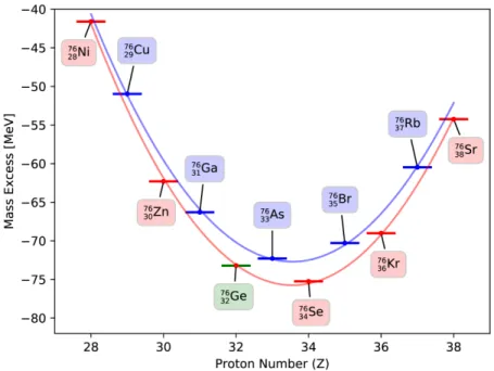
1.3 Isobar along even isobar A=76.76Ge is unable to single beta decay because both Ga and As would be energetically forbidden endpoints; double-beta decay of76Ge

to76Se is allowed, but highly suppressed. Data from [2]. . . 4

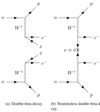
1.4 Feynman diagrams indicating the two forms of beta decay. . . 5

1.5 Feynman diagrams indicating double-beta decay . . . 10

2.1 A schematic of the MAJORANA DEMONSTRATOR, indicating the primary

experi-mental components . . . 15

3.1 Valence and conduction bands in a semiconductor, source [47]. The interatomic distance, orlattice constantais fixed for a given material, and the value it takes on

contributes to the exact band structure. . . 19

3.2 Germanium band structure diagram, adapted from [48]. . . 20

3.3 a) A single crystal being pulled from the melt in a czochralski-style pulling

appara-tus. b) The resulting boule following a czochralski pull. . . 22

3.4 The approximate PPC detector cross section as used by MJD. The HV conducting n+outer surface is indicated in pink, a nonconductive passivated surface in orange, and the small p+point-contact readout electrode in blue. The detector is axially

symmetric about the dashed line. . . 26

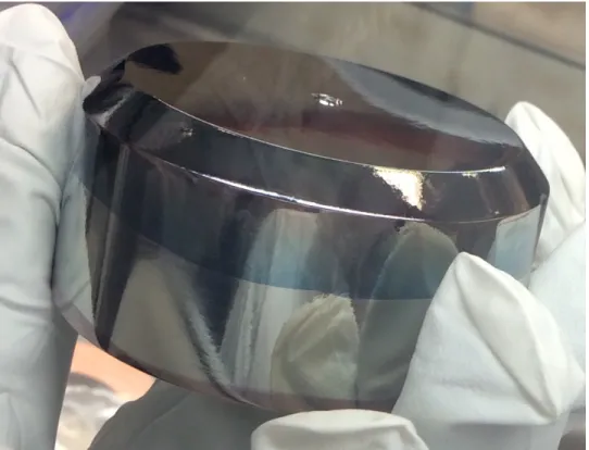
3.5 Photograph showing the “bottom” surface of an ORTEC enriched PPC detector.

Note the bevel and the small point contact. . . 27

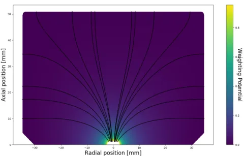
3.6 Simulated weighting potential, with lines indicating the drift trajectories. . . 30

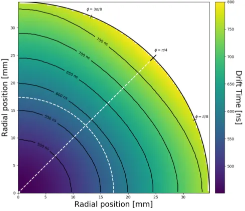
3.7 Simulated hole drift time map across a detector cross section. Shown for detector P42575A, at a constant z position of half the detector length. Note that the drift time contours are not azimuthally symmetric, with longer drift times atφ=π/4

for a given radius. The map is symmetric aboutφ=π/4. The hole drift time along

the white constant-radius curve is shown in Figure 3.8. . . 32

3.8 Simulated hole drift time along axis angleφ. Shown for detector P42575A, at a constant z position of half the detector length and a constant radius of half the detector radius. This corresponds to the drift time along the white dashed

3.9 Time domain waveforms from charges in a single cloud of gaussian with FWHM of 1 mm from the bulk of an enriched detector. This charge cloud is exaggerated for visualization. The gaussian cloud compares well to a smoothed waveform with

a gaussian kernel standard deviation of approximately 10 samples. . . 35

3.10 Color indicates the maximum difference in time at the 50 percent timepoint between waveforms in a cloud, at each point over the detector cross section. Detector is an

enriched ORTEC detector, so the bevel and point contact are visible. . . 37

3.11 Color indicates the maximum difference in time at the 50 percent timepoint between waveforms in a cloud, at each point over the detector cross section. Detector is a

BEGe, so the ditch outline is visible, with some edge effects. . . 37

3.12 A high-level schematic overview of the MJD signal readout chain. . . 38

3.13 Regions of signals waveforms discussed in this chapter. The waveform is a voltage

signal in the time domain. . . 40

3.14 The electric field viewed cross-sectionally inside one ORTEC geometry (enriched)

PPC detector (P42575A). The highest field location is near the point contact. . . 45

4.1 The distributions sampled by both Classic Nested Sampling and Diffusive Nested Sampling as the chain proceeds forward. The Diffusive Nested Sampling algorithm

allows for continuous mixing at shells of lower likelihood. Adapted from [90] . . . 55

4.2 Data structure for training fits. Other parameters (such as detector geometry) are not allowed to float. When fitting a single waveform, the fit uses the shared detector parameters without floating them and the single waveform parameters are fit to

match that waveform. Electronics models are indicated in Table 3.6.3. . . 60

4.3 Waveform fit comparison for an average waveform. The horizontal scale indicates a time parameter. The vertical scale on the top figure is a voltage, and the bottom figure indicates the residual difference between a data waveform and the proposed simulated value. The data and fit overlap considerably, with a residual feature at

the rising edge. . . 63

5.1 Beginning of level exploration for a fit using 105 particles per each of 4 waveforms over 750 levels. Each level is successively made, compressing the remaining prior mass in each subsequent level, and after all levels have been created, the particles

diffuse into exploring through all existing levels. . . 67

5.2 Top figure shows the log-likelihood as a function of the enclosed prior mass. Bottom figure shows the weights of the saved particles, shown by their enclosed prior mass values; particles to the left of the peak are not expected to contribute to

5.3 Fit result of impurity at each end of the detector for detector P42575A in dataset 1. The right plots are chains of the posterior values with the mean indicated, plotted as a function of sample number. The left plots are KDEs of the indicated chain,

with the median and mean estimates indicated. . . 68

5.4 Fit result of impurity at each end of the detector for detector P42575A in dataset 1. The three different colors each represent a training fit using 4 different waveforms,

and the black line is the average of the posterior maxima. . . 70

5.5 Comparison of energy parameters between fit data and trapezoidal filter estimation. The two metrics are largely in agreement, although some waveforms differ by as

much as 10 keV. . . 71

5.6 Comparison of energy parameters between fit data and trapezoidal filter estimation,

in a joint KDE plot centered over the 2615 keV photopeak. . . 72

5.7 Fitted positions for 112 calibration events in a single detector. Note that radius value is squared to correct for the cylindrical volume element. Events show some higher density near the radial extreme of the detector and some clustering in a small region near the surface. The events which have slower drift times are found

to correctly be located farther from the point contact (r = 0,z= 0). . . 73 5.8 Simulated event interaction locations for 630,525 calibration source events in

detector P42575A, with each blue point indicating a different event. Note that radius value is squared to correct for the cylindrical volume element. A higher color density indicates a relatively higher number of events in that location. Events show some higher density near the radial extreme of the detector and the density

decreases with increasing axial position. The event distribution is otherwise nearly uniform. . 74

6.1 Frequency response of forward and inverse transfer functions. The forward and inverse filters are nicely matched, indicating that much of the frequency-space

power can be recovered. . . 77

6.2 Waveform with electronics effects removed. Note that the falling edge of the

waveform is corrected to a flat top, as expected. . . 78

LIST OF ABBREVIATIONS

ADC Analog-to-Digital Converter

BEGe Broad Energy Germanium detector

CC Charged Current

CPU Central Processing Unit

DL Discovery Limit

DAQ Data Acquisition

DNest Diffusive Nested Sampling

DNS Diffusive Nested Sampling

FEniCS Finite Element Computational Software

FWHM Full width half maximum

GPU Graphics Processing Unit

HDF Hierarchical Data Format

HPGe High-purity germanium

I/O Input/Output

KDE Kernel Density Estimator

LBL Lawrence Berkeley National Laboratory

LNGS Laboratori Nazionali del Gran Sasso

MCMC Markov Chain Monte Carlo

MJD MAJORANA DEMONSTRATOR

MSPS Mega (106) samples per second

MVC Model-View-Controller

NC Neutral Current

NIB NeXT Interface Builder

NS Nested Sampling

ORCA Object-Oriented Realtime Control and Acquisition

ORTEC Oak Ridge Technical Enterprise Corporation

PDE Partial Differential Equation

PPC P-type Point Contact

QCD Quantum Chromodynamics

QDC Charge-to-digital converter

QED Quantum Electrodynamics

SBC Single Board Computer

SNO Sudbury Neutrino Observatory

SNR Signal-to-noise ratio

SPICE Simulation Program with Integrated Circuit Emphasis

VME Versa Module Europa

LIST OF SYMBOLS

a Isotopic Abundance

A Atomic mass number

B Background Index

E Electric Field Magnitude

Esat Saturation Electric Field Magnitude

G0ν Neutrinoless double-beta decay phase space factor

gA Weak axial coupling constant

M0ν Neutrinoless double-beta decay nuclear matrix element L(θ) Likelihood of parameterθ

me Electron mass

hmββi Effective neutrino mass in double-beta decay

n Neutron

N Neutron number

NA Avogadro constant,6.02×1023

p Proton

T10ν 2

Neutrinoless double-beta decay half-life

Uαi The PMNS mixing matrix

vd Electron or hole drift velocity

W molar mass

Z Atomic number

Z(θ) Model Evidence

α Fine-structure constant

β Equal weight enforcement hyperparameter in DNS

∆E Energy resolution

Detection Efficiency

Γ Decay rate

λ Backtracking scale length hyperparameter in DNS

µsat Saturation charge mobility

π(θ) Prior probability of parameterθ

CHAPTER 1 Introduction

1.1 Overview

Neutrinos are neutrally charged fundamental particles of very low mass, which interact only via the

weak nuclear force and gravity. Despite being ubiquitous in the universe, these particles have only minimal

interactions with matter, and their presence has proven to be an interesting field of study for generations of

scientists.

Experimentally, neutrinos are among the most challenging particles to detect, and the technology to detect

them has been an intentional and concerted development since they were first theorized. Due to their low

interaction rate, specialized, large volume detectors must generally1be used to detect the particles. Neutrinos

contribute in important ways to many nuclear processes, however, and their presence can be indirectly noted

even without these specialized detectors, as in the case of beta decay.

Theoretically, neutrinos have many interesting and unique characteristics that make them worthwhile to

study. They are the only massive fundamental particles to have no electric charge, so their exact properties

are somewhat uncharted territory; indeed, charged leptons such as the electron are detected and manipulated

primarily through their electromagnetic interactions. Their vanishingly small (but nonzero) masses have

forced physicists to consider the mechanisms that grant them mass, which are likely to be different from the

mechanisms in other particles. Neutrinos also take part in the unusual phenomena of flavor oscillation and

matter effects.

In addition to all this, neutrinos are viewed as a possible mechanism for the observed matter-antimatter

asymmetry in the universe. During the big bang, it is believed that matter and antimatter should have been

created in equal parts; today, however, we live in a matter dominated universe, devoid of any obvious pockets

of antimatter. This baryon asymmetry may be explainable through a lepton asymmetry if neutrinos are their

own antiparticles, violating lepton number. This possibility will be discussed further in section 1.5.

Figure 1.1: Chart of nuclides, indicating the dominant decay mode by color [1]. The line of stability zig-zags through the middle of the isotopes, near theZ=N line at low mass.

1.2 Beta decay

There are several common types of radioactive decay, including forms which release electrons, photons,

or alpha particles, as well as nuclear fission which often produces lighter nuclei. When neutrinos are created,

it is always by nuclear reactions involving the weak force, such as beta decay.

Figure 1.1 shows the table of nuclides, which indicates all the combinations of protons and neutrons that

can be combined to form nuclei and, in this version, the dominant decay mode for each isotope. The number

of neutrons and protons in a nucleus is approximately equal at low mass (A), but at higher masses all nuclei

are neutron-rich. If all the isotopes along a given isobar (constant A = N + Z) are viewed together by stability

(or mass excess), you get an approximately parabolic trough of nuclei with the most stable nuclides at the

bottom. This stable bottom corresponds to the black line of stability in figure 1.1, with beta decays funneling

inwards towards the line of stability.

When viewed in such an isobaric “cross-section” the bottom corresponds to the line of stability in the

table of nuclides, and isotopes with a higher or lower number of protons will decay inwards towards the line

Even numbered isobars, as 76 is, have an additional effect, rather than lying on a simple parabola. A nucleus

is more stable with an even number of protons or neutrons, or even more so with both. Nuclei with an even

number of neutrons or protons experience a pairing force which increases stability. For this reason, along the

even isobar in Figure 1.3 the stability zig-zags along Z as the isotopes vary from being even-even to odd-odd,

but this is not seen in odd isobars like Figure 1.2, where there is always one unpaired nucleon.

Beta decay often occurs in neutron- or proton-rich isotopes, (away from the line of stability), moving

them towards greater stability. A beta decay may occur in one of two ways, a positive or negative version:

p → n+e++νe (1.1)

n → p+e−+νe, (1.2)

the former equation being aβ+decay (in proton-rich isotopes), and the latter aβ−decay (in neutron-rich isotopes). This type of decay is particularly interesting because it is capable of transforming one type of

nucleon into another, a process which is otherwise not possible in nature – in a nucleus, this is quite literally

transmuting an atom of one element into another. In addition to this change, the emission of an undetected (and

therefore, effectively experimentally invisible) neutrino was a puzzle for early experimentalists, who, unable

to see all three decay products, struggled to reconcile the decay with energy and momentum conservation.

In 1930 Wolfgang Pauli correctly proposed that the existence of an unmeasured light neutral particle – the

neutrino – could explain the experimental results [3], but it would be decades later before such a particle was

directly measured.

1.3 Weak interactions

The weak force is mediated by three types of bosons, two charged, and one neutral. There are nine2weak

interaction vertices, and they can be categorized as eithercharged current(CC) orneutral current(NC) [4]. A neutral current reaction is one in which the exchanged boson is neutral (the Z0particle), and therefore has

no exchange of electric charge between the vertices. Similarly, a charged current reaction is one in which the

2_{I count these as (1) CC with a lepton and neutrino, (2) CC with two quarks, (3) Z}0

Figure 1.2: Isobar along odd isobar A=75. Data from [2].

n

p

νe

e− W−

(a) Beta-minus

p

n

νe

e+ W+

(b) Beta-plus

Figure 1.4: Feynman diagrams indicating the two forms of beta decay.

exchanged boson is charged (the W+or W−), and does exchange electric charge between the vertices. The

difference between these reaction types is easiest to see in the context of some examples.

A beta minus decay, for example, converts a neutron into a proton, an antineutrino, and an electron. In

Figure 1.4(a), you can see a neutron decaying into a proton, with emission of an electron and an antineutrino.

As the decay starts with an electrically uncharged particle and ends with a charged particle in the same vertex

(the neutron decaying to a proton), the connecting boson must carry some charge (theW−).

Each fundamental particle can be assigned somelepton numberL, which is+1for lepton particles (electrons, neutrinos, etc),−1for lepton antiparticles (positrons, antineutrinos, etc), and0for particles which

are not leptons. Beta decay conserves electric charge as well as total lepton number; both quantities are

conserved for all observed decay modes thus far. We will revisit the idea oflepton number conservationlater in this chapter.

Some interaction modes (such as a neutrino scattering with a charged lepton) can occur as either a NC or

CC interaction (and may then have an enhanced total likelihood of occurring).

1.4 Neutrino properties

The neutrino cross section is quite small, making interactions with other matter unlikely. The cross

section is primarily small because of kinematics of the decay; the virtual W and Z0 bosons are very heavy.

After several earlier attempts, the neutrino was first measured by Reines and Cowan in the Savannah

River Experiment [5]. Here, three large tanks of liquid scintillator were placed in close proximity to a nuclear

proton in the scintillator, producing a neutron and positron, as indicated by

¯

νe+p→n+e+. (1.3)

The signatures of neutron capture and positron annihilation in near-coincidence provided good evidence that

the neutrino had been captured on a proton. Due to its clear signature, thisinverse beta decayreaction has gone on to become a component of nearly all subsequent neutrino detection measurements.

Following this, the community experienced the Solar Neutrino Problem, first born out of an experiment

by John Bahcall and Raymond Davis. Here, Bahcall was responsible for a theoretical model of solar neutrinos,

explaining the nuclear reactions in our sun and determining the associated rates and energies of released

neutrinos [6]. Davis attended to the challenging experimental details of trying to actually measure solar

neutrinos [7]. The experiment came up with only about one third of the expected number: this was the Solar

Neutrino Problem. There were many theories as to the cause, varying from experimental mistakes to other

theories of the solar model. By 1998, Super-Kamiokande had shown some indications of flavor changing

[8], but with some ambiguity to the mechanism3. In addition, the gallium based experiments SAGE and

GALLEX/GNO had sensitivity to the low energy proton-proton fusion neutrinos (p-p), and had seen a deficit

of solar neutrinos [9]. The solar neutrino problem was finally resolved by the Sudbury Neutrino Observatory

(SNO) in 2001, verifying a model theorized by Bruno Pontecorvo in 1967 [10]. This experiment was able

to measure all three flavors of neutrinos, and could then see that some of the neutrinos created as electron

neutrinos in the sun hadoscillatedinto other flavor states by the time of their measurement.

As well as this, we know that the neutrino is a spin-1/2 particle4, it weighs much less than an electron but

has mass, and it can be produced in beta decays. Cross sections are modestly well known, and we can predict

many neutrino-related reaction rates [11].

Despite having decades of study, there are still some fundamental questions about the properties of the

neutrino. Perhaps the most important examples are that we do not know the value of the neutrino’s mass, nor

if it is a Dirac or Majorana particle – a distinction which will be discussed later.

Measurement of the neutrino’s mass evades more traditional measurement techniques. The neutrino is

the only known fundamental particle having mass but no electric charge. A charged particle can, for example,

3

Super-Kamiokande had sensitivity to both theνeflavor via CC reactions, and to all flavors via NC/scattering, but could not

distinguish between them.

be accelerated in an electric field to inform about its mass; this option is not available for the electrically

neutral neutrino. Additionally, the neutrino is stable against decay, preventing us from looking at its decay

products to infer its energy and momentum.

From neutrino oscillation experiments, we have confidence that the neutrino has mass. Additionally, these

experiments can tell us the relative mass difference between the three neutrino mass states. Cosmological

measurements from PLANCK currently place lower limits on the sum of all three mass states toP

mν <

230−540 meV [12]. While every experiment is somewhat model-dependent, these measurements are

arguably more-so, as they rely on a detailed understanding of how the universe evolved and how neutrinos

contributed to the formation of structure along the way. Measurements therefore must rely on only the present

universe to infer what may have happened during the previous 13 billion years, with (reasonable) models to

interpret what we see now.

Despite this knowledge that neutrinos have mass, we do not, however, know the mass ordering, nor the

absolute mass scale of neutrinos. That is, we do not know which of the three known mass states is heaviest,

and while we know how far apart the mass states are from each other, we don’t know how far the lightest

neutrino mass is from zero.

As a result, determination of the neutrino mass must come from other sources5. There are several

proposed (and in progress) experiments to resolve these issues. A direct, ”model-independent” way to

determine the neutrino mass is by looking at the spectral endpoint in beta decays, which has slight variation

for different neutrino mass values [13]; this is the strategy being employed by KATRIN [14] as well as Project

8 [15], although using very different experimental techniques.

1.4.1 Baryogenesis via Leptogenesis

While matter and antimatter are in many ways similar to each other, particles of each have opposite

quantum numbers, such as electric and color charges. The antiparticle of the familiar electron is the positron,

having identical mass and opposite electromagnetic charge (and lepton number). As far as is known today,

the universe consists almost entirely of matter, and not in any substantial way of antimatter [16]. In general

5

matter and antimatter are conserved quantities, and in a particle reaction the baryon and lepton numbers

remain constant6.

It is of interest then to identify mechanism which may be responsible for generating this matter-antimatter

asymmetry. One appealing mechanism of baryogenesis is via leptogenesis, where an excess of leptons

leads to an excess of baryons, however, this just pushes the problem to a different unexplained excess. The

Sakharov conditions are a set of conditions for producing matter from equal amounts of matter and antimatter.

These are:

Baryon number violation: Could be via leptons.

C and CP Violation: To distinguish matter and antimatter.

Out-of-equilibrium period: To prevent the asymmetry from reverting immediately back.

One theorized process which results in a net creation of matter is neutrinoless double-beta decay,

described in the following section.

1.5 Double-beta decay

An isotope which is forbidden from beta decaying may instead, in some cases, double-beta decay. This

decay is usually described as one of

2n → 2p+ 2e−+ 2νe, (1.4)

(A, Z) → (A, Z+ 2) + 2e−+ 2νe, (1.5)

and is a single nuclear event consisting of two simultaneous beta decays. In the even A=76 isobar shown in

Figure 1.3,76Ge is unable to single beta decay because both Ga and As would be energetically forbidden

endpoints; two-neutrino double-beta decay of76Ge to76Se is allowed by the standard model, though highly

suppressed. This decay is theoretically possible in 35 isotopes [17], and has been directly measured in 9

isotopes, with half-lives ranging from1018to1021years [18].

A related process which is interesting for several reasons is a rare decay mode known asneutrinoless double-beta decay. This process is theorized to be possible in some models, but has never been observed.

6_{This is not true in kaon decays, however, it is an indirect CP violation, and of insufficient magnitude to explain the observed matter}

The decay converts two neutrons within a single nucleus into two protons and two electrons, without the

release of any neutrinos, as in

2n → 2p+ 2e−. (1.6)

As the protons are bound in the nucleus, the two electrons receive the majority of the energy in the decay,

and their summed energy is nearly constant; this means that electrons in this decay would contribute to a

monoenergetic peak when measured together.

For this neutrinoless decay to occur,total lepton numberwould be violated, as it would prevent emission of two electron antinuetrinos (both haveL = −1, and their nonexistence in the final state would violate lepton number by∆L= 2). This would indicate that neutrinos are their own antiparticles, a class of particle

referred to as Majorana particles [19], as well as demonstrating that lepton number is not a conserved quantity.

This is in contrast to the more standard Dirac particle, which has a distinct particle and antiparticle. Since the

neutrino is fundamental and lacks electrical charge, it is conceivable that the particle and antiparticle are the

same object. Indeed there are no comparable fundamental particles from which we might infer otherwise.

As neutrally charged fundamental particles, the difference between neutrinos and antineutrinos appears

to be just an opposite chirality; this is an intrinsic property, like total spin. In light of the fact that neutrinos

have mass, this statement is effectively just noting that neutrinos and antineutrinos have opposite helicity (a

state property, like the observable spin projection). As a massive particle is necessarily traveling slower than

the speed of light, it is in principle possible for another particle to gain more speed, and pass it; from this

boosted reference frame, the neutrino momentum would be going the opposite direction, and the helicity

would be flipped. So, if the only difference between a particle and antiparticle state of a neutrino is helicity,

then the two states should be (at times) equivalent and interchangeable.

Efforts to measure the postulated process of neutrinoless double-beta decay have placed only limits

rather than measuring the process, even after a number of efforts over several decades. The process is highly

suppressed, and based on current experiments has an expected half-life of more than1025years in most

isotopes, and greater than1026_{years in}136_{Xe [20].}

A decay rate can be estimated using Fermi’s Golden Rule, which, for this decay is usually stated as

Γ =

T01ν 2

−1

=G0ν(Qββ, Z) M0ν

2

n n p e− e− p ¯ ν ¯ ν W+ W+

(a) Double-beta decay. n n p e− e− p W+

ν ≡ν¯

W+

(b) Neutrinoless double-beta de-cay.

Figure 1.5: Feynman diagrams indicating double-beta decay

which assumes the decay proceeds via light neutrino exchange. Here,Gis a phase space factor,M0ν term is anuclear matrix element(or “transition amplitude”), andmββis the effective neutrino mass.

The phase-space factorG0ν _{modifies this transition amplitude with information about the final energy} and momentum. This factor is in principle exactly calculable for a given isotope [21]. A decay from a

heavy primary into a light final product has many different ways to arrange the energy and momentum (so

has a large phase-space factor), but a decay from a light primary into a light final product does not give as

many options for how to arrange the energy and momentum, and so is phase-space suppressed. Additionally,

increasing the number of particles in the final state decreases the available phase-space (and therefore the

magnitude of this factor) due to the increased sharing of energy and momentum.

The nuclear matrix elementM0ν is a statement about the likelihood of the transition from one quantum state into another. It is effectively a measure of how much the wavefunctions for each state overlap.

Calculation of this value is extremely nontrivial (especially for heavier nuclei off of closed shells), and

estimates of the dimensionless quantity vary between about 3 and 6 for76Ge, due to differences in techniques

and assumptions; this difference is large and the nuclear matrix element enters the rate squared, amplifying

the effect. In order to perform the calculation, the initial and final state nuclear wavefunctions must be

for calculating nuclear matrix elements, including nuclear shell model, energy-density functional theory

(EDF), quasiparticle random phase approximation (QRPA), and the interacting boson model (IBM). In order

to reduce some of the uncertainties associated with this value, other related nuclear structure measurements

are being made [22]. For a current description of the challenges associated with double-beta decay nuclear

matrix elements, see [23] and [24].

While not shown in Equation 1.7, the weak axial coupling constantgAis often included such that the nuclear matrix element is explicitlyM0ν _{= g}2

AM. There are phenomenologically interesting reasons to consider why the axial coupling constant may be renormalized inside the nucleus to one of several possible

values [25]. This intrinsically produces some uncertainty in the scale of the value, amplified bygAappearing to the fourth power inΓ. IfgAis excessively quenched, the decay half-life could end up excessively large [26], leaving the reaction even more difficult to measure.

The effective neutrino mass accessible in a double-beta decay,hmββi, is the mass-weighted sum over the Leptonic Mixing Matrix7Uαi, expressed as

hmββi= 3 X i=1 U_ei2mi

. (1.8)

The hmββi term in the rate contains the leptonic part of the full matrix element, leaving the remaining (hadronic) processes to theM0νterm [27, pg. 173],[28, pg. 164]. As the rate is proportional to the (small but nonzero)hmββi, the rate is then “automatically” encoded with the requirement of nonzero neutrino mass directly. The full value of the term is

hmββi= c

2

12c213m1+s212c213m2eiα+s13m3eiβ

(1.9)

wheresij indicatessin(θij)andcij indicatescos(θij), withαandβthe complex Majorana phases. Neutrino mass eigenstates are not simultaneous with neutrino flavor eigenstates. The three neutrino flavor eigenstates

correspond to thee,µ, andτ particles, with each corresponding to a mixture of mass eigenstates1,2, and3, as

|ναi=

3

X

i=1

U_αi∗|νii (1.10)

The anglesθij are then the mixing angles that describe

The components of thishmββiterm are mostly modestly well known from oscillation experiments, and limits can be placed from cosmological observations as well [29]. There is no experimental knowledge of the

Majorana phase terms, and limits onhmββiare usually placed by allowing the phase angle values to float on the range[0,2π]and using the resultant range of outputs. Themiterms are not known, but limits can be stated.

In addition to this light-neutrino exchange mechanism, there are other possible ways for the decay to

proceed, such as by a heavy particle exchange or a mixture of heavy and light particle exchange. Measurement

of neutrinoless double-beta decay is generally agnostic to the mechanism, although some techniques which

are sensitive to the angular correlation or energy distribution of the final state electrons may be informative,

as in the SuperNEMO experiment [30]. The “standard” light neutrino exchange is favored, as higher order

effects may washout, leaving it an ineffective baryogenesis mechanism [31]. Regardless of which mechanism

is responsible, if a neutrinoless double-beta decay is observed, the neutrino must have Majorana mass and is

then a Majorana fermion [32, 33].

The observed quantity for a neutrinoless double-beta decay experiment is either a decay rate or a limit on

the minimum value of this rate. After a measurement, Equation 1.7 can be rearranged to give the effective

mass (assuming a particle lepton-violating mechanism). As different isotopes have different matrix elements

(and event rates), the uncertainty and model dependance can be improved by combining results from multiple

isotopes.

1.6 Sensitivity to double-beta decay

In the design of a neutrinoless double-beta decay experiment, it is important to consider what aspects will

improve the sensitivity to measuring double-beta decay. Sensitivity is a measure of the ability to recognize a

signal with some certainty in the possible presence of background signals.

The number of counts expected in the region of interest (ROI) for a counting experiment is given by

N =ln(2)

aM NA

W

| {z }

available nuclei

t T0ν

1/2

!

(1.11)

for isotopic abundancea, molar massW, and elemental massM, with detection efficiency, for a half life of

The sensitivity of an experiment is related to the number of counts, and is usually defined in one of two

ways, depending on whether backgrounds contribute to the measurement or not, as

T₁0_/ν₂∝       

aM t, background-free. a

q M t

B∆E, with backgrounds

(1.12)

with background indexBand energy resolution∆E[27, pg 197],[28, pg. 171][24, 34, 35]. The distinction between these is somewhat nontrivial, as they are not limiting cases of one another. The transition between

cases with and without backgrounds depends on the expected background rate. A low-background experiment

is defined by the number of background counts it receives; a background with a lower rate will require more

total exposure to accumulate enough counts to worsen the result. See [36, 37] for more details.

FurthermoreDiscovery Limit (DL) orDiscovery Potentialis a quantity which specifies the ability to not just set a limit, but to credibly make a measurement. After all, we would like to eventually make

measurements of physics, not just continue to set limits. A DL has two basic required components, a level of

confidence you require (Nσ), and a nonzero number of counts that you could credibly be expected to measure [37]. The DL will be a lower limit than the sensitivity, and is a more realistic picture of the usefulness of a

particular experiment.

When faced with the possible isotopes which may undergo double-beta decay, there are several metrics

to use to evaluate which is most ideal to actually measure. There are basic physics metrics, such as the phase

space factor and theQββendpoint energy value, which can give an estimate of the expected count rate for a given isotope and spectral feasibility. Also important is the expected nuclear matrix element magnitude [38].

Perhaps the most compelling arguments are the experimental realities of trying to build scalable, efficient

detectors using or containing the isotope of interest.

The isotope chosen by the MAJORANAcollaboration is76Ge. As will be discussed in the following chapters, germanium is also an ideal material for the construction of high resolution detectors; germanium

detectors are a standard nuclear physics spectroscopy tool for this reason. For a recent overview of other

CHAPTER 2

TheMAJORANADEMONSTRATOR

The MAJORANADEMONSTRATORis a germanium detector array experiment with the goal of evaluating methods to be used for a large-scale neutrinoless double-beta decay experiment. The approach is intended to

be modular and scalable. It consists of 58 detectors together weighing 44 kg distributed between two different

cryostat modules, referred to as Module 1 and Module 2.

There are many constraints when designing detector systems for a double-beta decay experiment. The

guiding principle is that radioactive backgrounds must be reduced as much as possible while increasing

the exposure and improving the energy resolution as well. Backgrounds are kept low through a careful

and deliberate program of radioassaying all components to be used near the detectors [40], and simulating

the potential impact each would have on the final result [41]. The MAJORANA collaboration underwent a significant and successful effort to electroform and machine high-purity copper underground to reduce

backgrounds and cosmogenic activation. Copper parts are used extensively to support the detectors and build

all close structural components, as copper is machinable and strong, yet has no natural radioactive isotopes,

and can be made very radiopure.

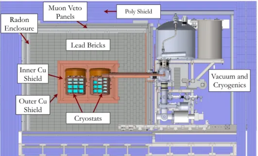
To shield from radioactive background sources near the detector array, the experiment uses a dense,

compact shield consisting of 54 tonnes of lead bricks surrounding inner layers of clean copper; theinner copper shieldwas electroformed and machined underground [40]. The lead shielding is surrounded by borated polyethylene plastic sheets, which can shield against neutrons. The inner volume is then flushed with

liquid nitrogen boiloff gas, which contains lower levels of radon than air.

The background constraint limits the number and type of electrical cables which can be used near the

detectors, and requires that most of the preamplifier circuit is outside the vacuum system. Signal and high

voltage cables are chosen to have low mass, an unusual constraint1. It is also desirable to have the most active

Figure 2.1: A schematic of the MAJORANADEMONSTRATOR, indicating the primary experimental compo-nents

detector mass with the smallest number of readout channels, as additional channels encumber additional

cables; this leads to development of large mass, single electrode detectors.

Many materials which are springy yet conductive contain low levels of radioactivity. As most electrical

connectors rely in some way on the elasticity of pins and sockets to force contact when meshing together, it is

difficult to form reliable, low-background connectors, especially over a broad temperature range. This process

was a major design effort for the collaboration, perhaps surprising to those outside the low-background

community.

An underground location is ideal as a way of shielding the experiment from cosmic rays (and cosmic

ray secondaries, such as muons). For this reason, the DEMONSTRATORis located 4850 feet underground at the Sanford Underground Research Facility, in the former Homestake Gold Mine, in Lead, SD. This is

the site of the well-known “Homestake Experiment” performed in the 1960s by Raymond Davis to measure

solar neutrinos [7]. The surface muon flux is2.0±0.2µ/s/cm2_{, and a measured flux at the site of the}

DEMONSTRATORof(5.31±0.17)×10−9 µ/s/cm2[42], corresponding to a reduction by nearly 9 orders of magnitude.

The detectors used in the DEMONSTRATORare made of germanium crystals (which are further discussed

in section 3.2). Our detectors are able to detect with high resolution the amount of energy deposited in them

To make the desired measurement, we have fabricated the detectors using germanium enriched in the

isotope76Ge, and are looking to observe the decay of the detectors themselves, with no external sources

present. This presents the advantage of capturing nearly all energy from events occurring within the detector,

and maximizing the detection geometry (nearly4π-coverage). It does have the curious feature of lacking

the ability to take “true” background datawithoutthe double-beta decaying source present, however, the expected rate is so small, this is in practice never a problem for the DEMONSTRATOR. An experiment with more modest resolution would struggle to differentiate between the endpoint2νββelectrons and any possible

0νββ electrons.

2.0.1 Status of the Demonstrator

The MAJORANADEMONSTRATORbegan commissioning on the first module in June 2015, followed by production data taking in January 2016; the experiment is currently taking data on both modules. In 2018, the

collaboration released its initial results from the full array, with blind data [43]. Here, we demonstrated an

energy resolution of 2.5 keV FWHM at the 2039 keV region of interest, and placed a lower limit on the half

life of1.9×1025_{years. More recently, we released another result, improving this limit to2.7×10}25_years

[44].

The DEMONSTRATORwas conceived of as an experiment to validate the feasibility of building a

larger-scale detector; the techniques being proposed had never been tried before and it is valuable to develop

experience with an intermediate-scale project before committing to a large-scale project. One issue that was

identified in the construction and operation of the experiment was that the cables and connectors to be used

can provide a number of reliability problems which reduced the yield of operational detectors.

2.0.1.1 Future of MAJORANA

In order to make a competitive measurement of double-beta decay, it is clear that a larger experiment is

necessary, and preferably one with further refined implementation. Although the MAJORANAand GERDA

collaborations are in principle competing to measure double-beta decay, the two groups have common

interests and experiences, and have worked closely together since their formation, with the goal of eventually

joining together into a single collaboration.

approach, which will demonstrate a medium-scale experiment of around 200 kg, followed by a full-scale

experiment at tonne scale. The design will be a hybrid of the technologies and strengths of each collaboration.

While detectors are currently being fabricated for this project, using the existing detector mass of the

DEMONSTRATORand GERDA projects can bootstrap the construction process and get the project started much more quickly. As a result, the DEMONSTRATORwill stop taking data and transition detectors into the LEGEND-200 cryostat located at Laboratori Nazionali del Gran Sasso (LNGS), in Assergi, Italy. As

there are naturally competing interests between prolonging the DEMONSTRATORand constructing the next generation LEGEND-200, the detailed timeline of this process is currently in flux.

2.1 Outline

The signals produced by the germanium detectors of the DEMONSTRATORare described in the following chapter. Using numerical simulations, we can simulate the expected fields and signals, given their dependence

on the detector geometry and characteristics.

Using a bayesian machine learning algorithm, we can use these simulations to estimate the actual

parameters of our detectors, as well as the individual waveform parameters (such as deposited energy and

hit position). In a training stage, we analyze a selection of non-simulated (data) waveforms from a single

detector to characterize the detector properties. Using a continuous feedback by simulating new fields and

signals, the waveforms are all simultaneously fit to give a best estimate of the common detector parameters.

After finding these values, they can be “frozen”, and individual waveforms can use this information to do a

CHAPTER 3 Signal Formation

Radiation detectors are devices which can convert ionizing radiation into a signal that is readily

mea-surable; there are many types of such detectors, each with various specific benefits and limitations. In

scintillators, radiation is converted to optical light, which can be measured with a light sensor. A bolometer

converts the deposited energy into thermal energy, which is measured with a temperature sensor such as

a thermistor. In a solid-state semiconductor detector, the radiation is converted directly into an electrical

current signal, measurable by the appropriate current-sensing instrumentation.

A germanium detector is a semiconducting single crystal often used to detect radiation. Ionizing radiation

incident on a crystal of germanium liberates electron-hole pairs, creating a small but measurable current

signal. The details of this process and the associated readout electronics necessary are subjects of this chapter.

Furthermore, we will discuss the techniques of modeling and simulating the signals from detectors.

3.1 Semiconductors

In 1931, Wolfgang Pauli famously proclaimed “One shouldn’t work on semiconductors, that is a

filthy mess; who knows whether any semiconductors exist.” [46] With the benefit of nearly a century of

additional study, we can now see that semiconductors have been one of the most fruitful avenues of scientific

investigation, and are responsible in some way for nearly all modern technology. They are also responsible

for a valuable technique in radiation detection, the semiconductor or solid-state detector.

A single atom has electronic structure, giving rise to specific allowed energy levels corresponding to each

electron’s quantized energy. When atoms are bound together at short interatomic distances in a crystal lattice,

the long range order of the lattice changes these levels to be bands, energy ranges in which the electrons may

occupy one of a more broad selection of energies, as shown in Figure 3.1. In reality, the bands are composed

Figure 3.1: Valence and conduction bands in a semiconductor, source [47]. The interatomic distance, or

lattice constantais fixed for a given material, and the value it takes on contributes to the exact band structure.

Of primary interest is the behavior of the electrons in the conduction and the valence bands. The conduction band electrons are the highest energy electrons in the material, and are loosely bound, not limited

to any particular lattice site. The valence band electrons are slightly lower in energy, and are bound to

particular lattice sites. The valence band is the highest energy filled band, and is completely filled in a

semiconducting material.

Germanium, like silicon and carbon, has 4 valence electrons. These 4 electrons are covalently shared

with adjacent atoms, most commonly forming a diamond cubic lattice, the same structures as formed by

silicon and carbon-based diamond.

In an electrical conductor such as a metal, the valence and conduction bands overlap in energy (there

is no gap), and the valence electrons can very easily be moved into the conduction band; by default, the

conduction “band” will already contain some electrons. In an insulator, there is a large gap between these

bands, and valence electrons require considerable energy to be elevated into the conduction band. For a

semiconductor, the gap is of a “moderate” size, and electrons may be pushed into this higher energy band

relatively easily. It is this mechanism that we will eventually describe as being useful for making radiation

detectors.

Electrons and holes feel some effective mass1while in the lattice, which will depend nontrivially on their

momenta and energy. An electron band structure diagram, as in Figure 3.2, shows the relationship between

the charge carriers’ energy and momenta (wavevectors), usually in a 2-dimensional representation of the

Figure 3.2: Germanium band structure diagram, adapted from [48].

4-dimensional (E,kx,ky,kz) space. This figure is also referred to as a dispersion relation. Such a diagram contains a significant amount of information about a material’s electronic properties such as the density of

states and band gap energy. The band gapEgof germanium occurs at the L point, along theh111idirection. As there are 8 equivalent h111idirections, there are 8 conduction band minima. Other conduction band

local minima include theΓ1andΓ2minima, though they are less important for this study. Other properties

can visually be deduced, such as the momentum necessary for the indirect transition between the band gap

minimum and the zero-momentum gamma point. Furthermore, the effective mass is inversely proportional

to d_dk2E2, the second derivative of the dispersion curve at a given point. As the electron and hole will be

in different bands, the two will in general have different dynamics. This is interesting, because, without

any knowledge of the electron or hole wavefunctions, we can still deduce the transport properties such as

instantaneous velocity and acceleration of an electron or hole in an external field [49]. This will be valuable

3.2 Germanium Radiation Detectors

Germanium radiation detectors are a class of semiconductor detectors, all which operate on a similar

principle. They are ubiquitous, well-established tools within nuclear radiation spectroscopy, and have been in

use for spectroscopy in various forms since the 1960s. They have several advantages over other technologies,

most prominently including their excellent energy resolution and timing characteristics [50].

The earliest solid-state detectors were simple, thin planar detectors and were primarily used for charged

particle detection. The primary use for germanium detectors in the 1960s and onwards was in gamma ray

spectroscopy. These detectors were mostly coaxial and semi-coaxial geometry detectors. In the 1980s, it was

realized that semiconductor patterning techniques could be used to make highly segmented detectors, with

many channels to be read out in parallel on the same single crystal. These segmented detectors were usually

silicon and had an increased complexity in operation, but with a high degree of spatial resolution, allowing

for different types of analysis of high value for some experiments. Additionally, by segmenting the detector,

the total signal rate in each segment is lower, which may be practically necessary for high rate applications

[51, pg. 318] Though their spatial resolution may help eliminate some background signals, their need for

more readout channels would introduce too much background near the detectors, so they are not currently

used for neutrinoless double-beta decay experiments. Additionally, segmented tracking detectors are often

designed to be lower mass reduce scattering, counter to the exposure needs of rare event searches.

3.2.0.1 Detector Processing/Fabrication

The basic germanium detector is a single monocrystal of germanium, often shaped in a right circular

cylinder. The crystals are of very high purity, and are usually grown by the Czochralski method. In this

method, a rotating seed crystal is slowly pulled from a melt to form a boule, as indicated in Figure 3.3. Usually

detectors are pulled with theh100icrystal axis along the pull-axis [52, pg. 19], thoughh111imay also be

used in some applications2. In general, cylindrical detectors have an unknown azimuthal axis orientation in

operation, as most spectroscopy applications are not able to see any effects from this.

In order to purify the material that is used for Czochralski growth, several important techniques are used.

After isotopic enrichment, the detectors are in a76GeO2form, which is then chemically reduced to form

the metal. This material is zone refined until it reaches a resistivity of at least 47 ohm-cm, equivalent to

2

1013electrically active impurities per cubic centimeter [53]. With this material, the detector manufacturer

further zone refines the material to at most1011impurities per cubic centimeter, then it is grown into a single

crystal by the Czochralski method which further eliminates impurities in the material; further discussion of

the consequence of these impurities will be found in the next section. Often, the final zone-refining step must

be performed after a first crystal growth, as this prevents impurities from collecting at the grain boundaries

inside the material [54]. After crystal growth, the boule is sectioned and adequate parts may be used for

detector fabrication, while others may be re-grown to further purify as needed. This crystal section will then

be machined into a detector geometry and patterned with contacts.

3.2.0.2 Impurities

The crystal may be doped with an “impurity” of some sort in order to give it the appropriate

semicon-ducting properties. While the term impurity may colloquially imply that it is undesirable, it should instead be

interpreted to mean that it is a difference from being a perfect lattice of germanium atoms; the impurity is one

of the most important properties in the manufacture of any semiconductor. These impurities may come from

simple lattice defects, such as a dislocation or vacancy, or they may come from an atom of an element with a

larger or smaller number of valence electrons than germanium taking a germanium atom’s place in the lattice.

Regardless of how it is achieved, the result is a relative lack or excess of electrons in the area localized near

the impurity. The intentional addition of a material into a semiconductor in this way is known as doping.

A doped semiconductor has an unequal concentration of free electrons and holes. A p-type semiconductor

has a majority of its free charge carriers as positive holes, whereas an n-type semiconductor has a majority of

its free charge carriers as electrons. Most commonly, group IV semiconductors like germanium are doped with

a group III element (usually boron) to make them more p-type or a group V element (such as phosphorus or

arsenic) to make them more n-type. High-purity germanium (HPGe) has very low concentrations of impurities,

with typical values being less than1010electrically active impurities per cubic centimeter, equivalent to parts

per trillion concentration (see Appendix A).

Normally the impurity levels at the tail and seed ends of the boule will not be the same, for a given

impurity type. This is because the solubility of impurities is different in the liquid than solid phase; the ratio

of the concentrations in the solid and liquid phases is known as the segregation coefficient for that impurity

type. Aluminum (a p-type impurity) has a segregation coefficient near 1, causing it to be nearly uniformly

distributed in the crystal. Several n-type impurities such as phosphorous and oxygen have segregation

coefficients less than 1, and will then be preferentially found in the liquid phase, corresponding to a higher

concentration in the tail end of the crystal (as they become concentrated while the crystal is pulled from the

melt). For this reason, HPGe crystals are usually p-type at the seed end and n-type at the tail [52]. While in

general this gives a predictable gradient of impurity concentration, material may also be introduced into the

melt while being pulled to change this behavior, as well as diffused into the material after growth. Usually

the details of what is done here are considered proprietary trade secrets. The impurity concentration gradient

is of great importance in germanium detector operation, and will be discussed further in later sections.

As only a very small impurity concentration determines the majority carrier type, it is possible when

growing a high-purity germanium detector to inadvertently produce the wrong type crystal. It is only by

detailed process control that high-purity detector production is made possible.

3.2.0.3 Contacts

Additionally, the detector must have contacts at the anode and cathode. This allows for the detector to

have a uniform potential over the relevant surfaces, as well as giving a location for readout. The presence of

Contacts come in two basic types, ohmic(or, non-rectifying) and blocking(also calledrectifyingor

non-injecting). Normally, a detector has (at least) one of each type.

The rectifying contact in a p-type detector is then+contact, which is dissimilar to the bulkpmaterial [50]. These contacts form a P-N junction, which is effectively low resistance under forward bias and high

resistance under reverse bias. A positive voltage is applied to then+contact, in the reverse bias configuration. In this way, a voltage can be applied to the detector (and in turn an electric field), which depletes the bulk to

form the active detector volume.

The non-rectifying contact in a p-type detector is thep+contact, which is held at 0 V, and is where the signal is read out from. This contact is effectively high resistance, and reduces the leakage current through

the detector. As both the bulk and the contact are p-type, this is not a semiconductor junction, but instead

current is blocked by the minority carrier motion[50]; that is, there simply are not enough minority carriers

(free electrons, in this case) in the material to propagate negative charge through the junction. The current

under bias of several thousand volts would then be unacceptably high without a blocking contact.

The area between the contacts must not be conductive, so as to avoid forming surface currents across the

detector which could mask the intended signal current through the detector. In silicon, the surface naturally

forms a robust oxide which is nonconductive. While germanium also readily forms a surface oxide film

when exposed to oxygen or water, the naturally formed germanium oxide is chemically inhomogeneous,

porous, and low-density, which can lead to charge accumulation along the surface of the passivation layer

[55]. Therefore, germanium must be carefully treated to form such a passivation layer, and there are many

(often proprietary) techniques for accomplishing this.

3.2.0.4 Operation

Germanium has a band gap of approximately 0.6 eV and an electron-hole creation energy of around 3 eV.

The difference between these values can primarily be understood as some energy being transferred to the

crystal lattice as phonons [56]. The germanium bandgap is relatively small among semiconductors, at roughly

half the value of silicon. The result of this small bandgap is that thermal energy at room temperature is

sufficient to excite electrons across the bandgap, creating a high leakage current. In order to circumvent this,

the detectors are operated at low temperature, usually using liquid nitrogen or mechanical cooling methods to

keep detectors around 80 K. Subsequently, the detectors must also be kept under vacuum, otherwise water

An alternative that has been investigated in the past is operating detectors directly immersed in a liquid

cryogen such as liquid argon; this is the technique used by the GERDA collaboration.

3.2.1 Signal Formation in a Detector

Ionizing radiation incident on a crystal of germanium will liberate electrons and holes in pairs. Having

opposite electric charge, these electron-hole pairs would normally just diffuse randomly in the crystal,

trapping on crystal defects or mutually attracting and recombining immediately. Instead, if a voltage is

applied across the detector, the electrons and holes (with opposite charges) will experience forces in opposite

directions, preventing recombination. These charges will drift in the applied electric field, inducing a charge

in a readout electrode, where the signal is read out.

It is possible to have several readout electrodes on a single detector. Additional electrodes provide

additional information about the position of the charges as they move through the detector volume.

The raw detector signal that is formed has a detailed dependence on the electric fields present, and

therefore also the detector geometry and impurity profile.

A useful quantity when considering signal formation by charges moving through a detector is the

weighting potential. The weighting potential is the solution to Laplace’s equation for a given detector geometry, with unit potential on the electrode of interest and zero potential on all other electrodes [57]. In a

multi-electrode detector, you would have several different weighting potentials corresponding to the signal

observed for each electrode; in this scenario there is increased utility in being able to calculate the expected

signal for each contact. In a single electrode configuration, where the readout electrode is held at ground, the

result is effectively a normalized electric potential.

3.2.2 Detectors for theMAJORANADEMONSTRATOR

The germanium detectors used by the MAJORANADEMONSTRATORare of a type known as P-type Point Contact (PPC) detectors. The point-contact germanium detectors were first developed by Luke et. al.

[58] as a way of fabricating large volume detectors capable of low energy threshold operation, for rare event

searches such as dark matter3. These detectors have a geometry which is approximately indicated in the

cross-sectional line drawing in Figure 3.4, and a photograph in Figure 3.5.