The selection of electrical analog components from computational model impedance spectra

THE SELECTION OF ELECTRICAL ANALOG COMPONENTS FROM COMPUTATIONAL MODEL IMPEDANCE SPECTRA

Lucy Perkins Phelps

A thesis submitted to the faculty of the University of North Carolina at Chapel Hill and North Carolina State University in partial fulfillment of the requirements for

the degree of Master of Science in the Joint Department of Biomedical Engineering.

Chapel Hill 2010

ii ABSTRACT

LUCY PERKINS PHELPS: The Selection of Electrical Analog Components from Computational Model Impedance Spectra

(Under the direction of Dr. Brooke Steele)

iii

DEDICATION

I would like to dedicate this work to a few of the people who have most supported me, through both my trials and successes, and that have helped me to reach this

point in my academic career:

My husband, Luke, who is my everything, My sister, Elle, who is my happiness,

iv

ACKNOWLEDGEMENTS

I would like to thank Dr. Brooke Steele, my advisor, for her patience and guidance throughout my time as a graduate student.

I would like to thank my committee, Dr. Carol Lucas and Dr. Shawn Gomez, for their support.

I would also like to thank Rachel, for being a student mentor who was always willing to help or talk things through.

v

Table of Contents

LIST OF TABLES ... viii

LIST OF FIGURES ... ix

ABBREVIATIONS AND SYMBOLS ... x

Chapter I. INTRODUCTION AND BACKGROUND ... 1

1.1 Motivation ... 1

1.2 Cardiovascular System ... 2

1.3 Computational Models of Systemic Circulation ... 5

1.4 Impedance ... 7

1.5 Lumped Parameter Models (Electrical Analogs) ... 9

1.6 Parameter Estimation ... 12

1.7 Specific Aims ... 14

II. METHODS ... 16

2.1 Gold Standard Impedance Spectra ... 17

vi

2.3 Intermediate Results ... 21

2.4 Final Studies-Impedance Spectra Estimations of Capacitance ... 25

2.5 Two-Element Lumped Parameter Model ... 27

2.6 Comparison of Fourier Domain Method to Time Domain Method ... 28

III. RESULTS ... 29

3.1 Three-Element Lumped Parameter Model ... 29

3.2 Two-Element Lumped Parameter Model ... 31

3.3 Comparison of Time Domain and Fourier Domain Method ... 33

IV. DISCUSSION AND CONCLUSIONS ... 36

4.1 Conclusions ... 36

4.2 Limitations ... 39

4.3 Future Work ... 40

APPENDIX I ... 41

MATHMATICA PROGRAMS ... 41

1. Three Methods of selecting R1, dynamically selecting C ... 41

APPENDIX II ... 46

MATLAB PROGRAMS ... 46

vii

viii

LIST OF TABLES

Table

ix

LIST OF FIGURES

Figures

1. Major Arteries of the Viscera and Lower Extremities ... 3

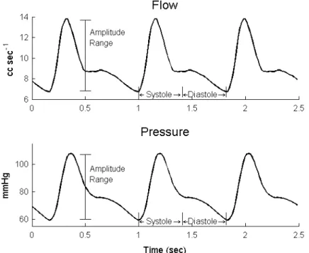
2. Typical Blood Flow and Pressure Waveforms ... 4

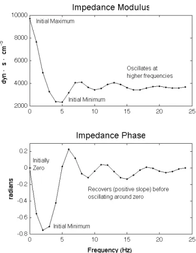
3. Typical Shape of Impedance Modulus and Phase ... 8

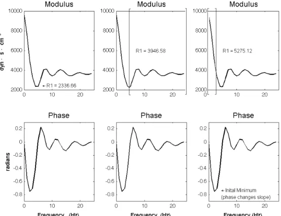
4. Two- and Three-Element Windkessel Models (Electrical Analog) . 10 5. Three Methods for Selecting the R1 Parameter ... 19

6. Effects of Changing C on Flow and Pressure Waveforms ... 20

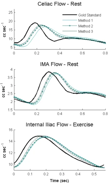
7. Examples of Flow Comparisons ... 23

8. Examples of Pressure Comparisons ... 25

9. Dynamically Altering C in the Two-element Lumped Parameter ... 31

10. RCR vs. RC ... 32

x

ABBREVIATIONS AND SYMBOLS

IMA Inferior Mesenteric Artery

P Pressure

Q Flow

CHAPTER I

INTRODUCTION AND BACKGROUND

1.1 Motivation

2 1.2 Cardiovascular System

The cardiovascular system is composed of the heart and the circulatory system. The heart acts as a pump, generating pressure that circulates blood throughout the circulatory system to the tissues and organs of the body. The circulatory system is divided into two circuits, the pulmonary circulation and the systemic circulation. The pulmonary circulation delivers blood from the heart to the lungs and back to the heart. The systemic circulation consists of the blood vessels that carry oxygenated blood throughout the rest of the body.

1.2.1 Systemic Circulation

Arteries are the blood vessels of the systemic circulation that carry blood away from the heart, delivering oxygen and nutrients. Arteries are composed of a thick smooth muscle layer and large amounts of elastic and fibrous connective tissue. Arteries form a branching pattern throughout the body, dividing into smaller and smaller arteries. Eventually these arteries become arterioles and capillaries, the smallest vessels in the cardiovascular system. The capillaries join with venules and are the site of gas and nutrient exchange for the systemic circulation. Then, oxygen poor blood returns to the heart via the body’s venous system [1].

3

Figure 1: Major Arteries of the Viscera and Lower Extremities - modified from figure

found at http://www.answers.com/topic/artery

1.2.2 Blood Flow

4

the body. However, it yields no insight as to how that blood is distributed throughout the arterial system. Hemodynamic models are useful in characterizing blood flow where experimental data cannot be extracted. Knowing the resistive and compliance characteristics of a particular arterial network allows insight about the blood flow and pressure through the vasculature in question. As previously mentioned, the arterial system forms a branching pattern throughout the body. As the size (radius) of the arteries decrease, the walls of these blood vessels become much less elastic [1]. This loss of elasticity, or compliance, combined with blood viscosity and the length of the blood vessels create the resistance to blood flowing through the branching arteries.

Figure 2: Typical Blood Flow and Pressure Waveforms- This figure shows the

5 1.2.3 Blood Pressure

Blood is propelled throughout the systemic circulation by the heart. The ventricles of the heart contract creating the pressure which drives blood through the arteries (Figure 2). Blood flows from high to low pressure and the flow is inversely proportional to the resistance of the blood vessels [1]. During exercise negative flow that exists during rest conditions is eliminated due to increased heart rate and cardiac output [6]. During exercise, cardiac output increases (going from approximately 5 L/min to 30-35 L/min for a healthy person with resting heart rate of 72 bpm) [1]. During rest or exercise, the geometry of arterial networks, changes in vascular anatomy (dilation or constriction of the vessels) and the resistive and compliance characteristics of vessels are all parameters that are considered in hemodynamic models that yield accurate representations of blood pressure and flow.

1.3 Computational Models of Systemic Circulation

6

Two types of boundary condition models that are extensively used for this application are geometric and lumped parameter impedance boundary conditions. Geometric, or anatomically based distributed models, represent a vascular network by assuming a specific geometry (such as a structured branching tree) and computing impedance [6, 7]. Lumped parameter models represent an arterial system as an electrical circuit inputting blood flow as current or blood pressure as voltage. Both types of models allow characterization of blood flow and pressure data for the circulatory system outside of the arterial network being studied, and are good boundary conditions for this application.

1.3.1 Boundary conditions

7 1.4 Impedance

8

Figure 3: Typical Shape of Impedance Modulus and Phase

9

makes impedance a good validating parameter for both lumped parameter and geometric models [9].

1.5 Lumped Parameter Models (Electrical Analogs)

10

Figure 4: Two- and Three- Element Windkessel Models (Electrical Analog) - a)

Two-element Windkessel model where R represents the total resistance and C represents the compliance of an arterial network. b) In a

three-element Windkessel Model the Zch is added to the circuit as a resistor.

The three-element Windkessel model adds the parameter of characteristic impedance, which is typically represented by a second resistor in the electrical analog. This is shown in Figure 4(b). The characteristic impedance (Zch) added to the peripheral resistance (R) comprises the total equivalent resistance. This characteristic impedance parameter allows the model to better represent the higher frequency characteristics, though the oscillations are still not present. This parameter is described as the wave speed multiplied by blood density divided by cross-sectional area (or Z_ch = γρ

11

characteristic impedance and overestimate the total arterial compliance [13, 14], the three element Windkessel is generally accepted to be a useful compromise between accuracy and complexity. In The Arterial Windkessel, Westerhof et al. [2] concludes that the three-element Windkessel model can adequately describe the pressure-flow relations at the entrance of a systemic arterial system.

Because low frequency errors can occur with the three-element Windkessel model, which can be attributed to the inclusion of the characteristic impedance, four-element models have been examined. Typically this includes an inertance in series with the characteristic impedance but this inertance was seen to be extremely difficult to estimate [2]. For the applications investigated in this project the two- and three-element models were deemed more appropriate.

1.5.1 Impedance of Windkessel Model

A lumped parameter or Windkessel model, representing a downstream arterial system, can be used as a boundary condition when modeling a larger vascular network. Typically a three-element model, the frequency-dependent impedance of such a boundary condition can be computed as seen in Equation 1 [14].

(

)

ω

+ +

=

+

1 2 1 2

2

0,

1

R R i CR R

Z

12

The impedance of lumped parameter models do not have the same shape as the aforementioned typical experimental impedance models as they lack the oscillations at higher frequencies (wave reflections).

1.6 Parameter Estimation

Parameter estimation for lumped parameter models has been extensively investigated. The peripheral resistance is typically represented as the initial ratio of pressure to flow [2, 15]. However there have been many ways of estimating the total arterial compliance and the characteristic impedance.

three-13

element model. Several other parameter estimation strategies are also described and the limitations and advantages of each are briefly discussed. All the strategies for estimating arterial compliance rely on measured pressure or flow data [2].

No current methods for estimating this parameter solely use Fourier domain data. Several sources do point out that compliance is a low-frequency property, so the best compliance estimation methods should utilize the lowest frequencies [13, 16].

The most accurate way of estimating the characteristic impedance has also been examined. Typically this parameter, characterized by a second resistor, is estimated by averaging input impedance modulus values over a particular range of frequencies [17, 18], though the definition of that range is somewhat ambiguous. It has also been approximated using slopes of pressure and flow waveforms during early systole [17].

One current limitation of using the lumped parameter boundary conditions is that the most accurate current parameter estimation strategies require experimental data. A particular focus of this work is to investigate parameter estimation strategies that require no time domain data, selecting all RC and RCR parameters from impedance spectra.

14

equations of the three-element Windkessel. These are shown in Equations 2, 3 and 4.

= 1

∑

( ) k ch k PPA t Z

m Q t (2)

= mean −

ch mean P R Z Q (3) − + = − − −

∫

∫

1 1

1 2 1 2

( ) ( ) ( )

( ( ) ( )) ( ( ) ( ))

t t

avg ch avg

t t

avg avg ch avg avg

P t dt R Z Q t dt

C

R P t P t RZ Q t Q t (4)

The accuracy of this method was examined by comparing it with four previously published methods. The pressure and flow waveforms were reconstructed using all methods of estimating the Windkessel parameters and were compared back to experimental flow and pressure waveforms [4]. It was concluded that this method performed as well as the other known strategies.

1.7 Specific Aims

15

CHAPTER II

METHODS

17

comparisons of both models are compared to previously established parameter estimation methods.

2.1 Gold Standard Impedance Spectra

In order to compare the different methods for selecting the RCR components, previously developed one-dimensional (1D) finite element analysis (FEA) software [19] was used to model the visceral and peripheral blood flow and pressure. The outlet boundary conditions were specified with structured tree parameters for each outlet for both rest and exercise conditions [6]. The impedance spectrum for each was then computed using Womersley’s method of calculating impedance for oscillatory flow in an elastic tube [20] and the structured tree parameters as described in detail by Olufsen, et al [6, 14].

18 2.2 Three Element Lumped Parameter Model

2.2.1 Estimation of Characteristic Impedance (R1)

A typical impedance modulus will have an initial maximum value (typically the zero frequency value or equivalent resistance), then will decrease to a minimum. After the minimum has been reached, the values will oscillate at higher frequencies for experimental and structured tree moduli spectra (such as in Figure 3) or exponentially approach the characteristic resistance for lumped parameter modulus spectra (such as in Figure 6).

Figure 5: Three Methods for Selecting the

resistor (R1) is set to a minimum modulus value

resistor (R1) is set to the average of the higher order modulus terms

minimum modulus value

average of the modulus terms up to the term in which the phase angle of the impedance spectra changes slope

2.2.2 Estimation of Peripheral Resistance (R2)

The equivalent resistance is the sum of the two element Windkessel model

taken directly from the impedance data, therefore once the estimated the R2 resistor was calculated.

19

Three Methods for Selecting the R1 Parameter: 5a) Method 1: the proximal

) is set to a minimum modulus value 5b) Method 2: the proximal ) is set to the average of the higher order modulus terms

minimum modulus value 5c) Method 3: the proximal resistor (R1) is set to the

modulus terms up to the term in which the phase angle of the impedance spectra changes slope

2.2.2 Estimation of Peripheral Resistance (R2)

The equivalent resistance is the sum of the two resistances in a three model (R_e =R₁+R₂). The zero frequency value can be taken directly from the impedance data, therefore once the R1 resistor was

resistor was calculated.

a) Method 1: the proximal b) Method 2: the proximal ) is set to the average of the higher order modulus terms after the ) is set to the modulus terms up to the term in which the phase angle of the

resistances in a three-The zero frequency value can be

20

2.2.3 Intermediate Methods -Dynamic Optimization of Capacitance

Once the resistance values were chosen, the capacitance values are selected by minimizing the amplitude error, reproducing accurate diastolic means, and replicating the wave shape between the reconstructed flow and pressure waveforms and the original data. Custom software allowed the dynamic altering of a capacitance value for error minimization, using the resistance values from each method described above.

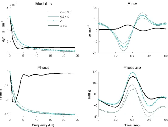
Figure 6: Effects of Changing C on Flow and Pressure Waveforms – Dynamic

selection of C allows for the important characteristics of the modulus and phase spectra to be identified. Recovery time of the phase curve increases accuracy of flow and pressure reconstructions (Example uses computed Celiac Flow data under rest conditions as the Gold Standard, where C (best

21

The capacitance value that minimizes the error between the original and the reconstructed pressure or flow waveforms as selected. The method with the lowest error was determined to be the best method for selecting the resistance components (or, optimizing error values by dynamically choosing C allows comparison of the selection methods of R1 and R2). This “best” method of selecting the resistance values can then be used in determining the features of the impedance spectra that are important for computing a capacitance value.

2.3 Intermediate Results

2.3.1 Determining Resistance Selection Method

22 2.3.2 Comparison of Flow Waveforms

23

Figure 7: Examples of Flow Comparisons – The flow waveforms reconstructed using

all methods are compared to the computed gold standard data. IMA and Celiac arterial flow under rest conditions and Internal Iliac flow under exercise conditions are shown as examples.

2.3.3 Comparison of Pressure Waveforms

24

25

Figure 8: Examples of Pressure Comparisons – The pressure waveforms

reconstructed using all methods are compared to the computed gold standard data. Iliac and IMA arterial pressure under rest conditions and Internal Iliac pressure under exercise conditions are shown as examples.

2.4 Final Studies - Impedance Spectra Estimations of Capacitance

26

negative slope before reversing to a positive slope. For an RCR phase spectrum, the phase angle will then exponentially approach zero, while an experimental phase angle may oscillate and become positive. By examining the impedance spectra that produced the most accurate flow and pressure reconstructions, several notable observations about the phase were made. These observations were used to identify important graphical characteristics of the “best” RCR impedance phases so as to help develop a method to best estimate a C value.

The reconstructed vs. original flow waveforms, illustrated that the recovery time of the impedance phase after the initial minimum is important and should play a role in capacitance value selection. Upon examination of several impedance spectra, it appeared that the intersection of an impedance phase produced by the “best” method of resistance selection and the original “gold standard” impedance curves would be approximately close to a value that minimized this settling time. So to estimate C, equation 5 was implemented in software.

ω ω

− − =

−

1 2

1 2 2

Z R R

C

27

Here ω _{is the chosen frequency (intersection of phase curves –} determined to be approximately 2/3 the peak to peak of the initial positive sloping phase), R1 and R2 are previously estimated and Z and Zi are the impedance modulus and phase values at the chosen frequency.

2.5 Two-Element Lumped Parameter Model

Though a three-element lumped parameter model is typically depicted as being superior to the two-element model for this application, the two-element Windkessel is simpler to implement. Therefore if it can achieve similar or even better results, then its usefulness may be re-evaluated. As this is a novel approach to parameter estimation, both two- and three-element Windkessel models are examined.

2.5.1 Estimation of (total) Peripheral Resistance (R)

As previously described, the two-element Windkessel Model excludes the characteristic impedance found in the three-element model. Here the resistance value is the initial ratio of the blood pressure to blood flow, or the first harmonic value of the impedance modulus (the initial maximum of a typical modulus). This is easily included in the software as zeroing the R1 term.

2.5.2 Estimation of Capacitance (C)

28

equations. In the two-element case this simplifies to Equation 6 where components are estimated as presented in the three-element case above:

ω

−

= R Z

C

Zi R (6)

These impedance moduli and phase, for the two-element model, will have a different typical shape than either three-element, or experimental impedance spectra. The impedance modulus will exponentially approach zero from the initial maximum, and the phase plot will not recover after reaching its initial minimum. Again, pressure and flow can be reconstructed from the estimated components and compared to the three-element model reconstructions and the “gold standard” data.

2.6 Comparison of Fourier Domain Method to Time Domain Method

CHAPTER III

RESULTS

3.1 Three-Element Lumped Parameter Model

3.1.1 Selection of Resistance Values – Intermediate Step

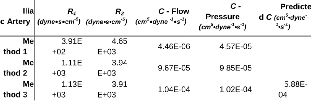
The best method of selecting the resistance components is validated in the intermediate step of the methods section. This determined that Method 3 is the most accurate at reproducing flow and pressure waveforms from a given impedance spectra using an optimized capacitance. Examples of the values chosen for resistance and capacitances for all methods are shown in Table 1.

3.1.2 Selection of Capacitance Values - Final Studies

30

Error, over all cases under rest conditions the amplitude range for blood flow is reproduced to within 8.4% and the amplitude range for blood pressure is reproduced to within 7.03%. After removing the aforementioned two outliers, these percentages decrease to within 5.4% for both blood flow and blood pressure reconstruction. This value (for pressure and flow) approximately doubles when comparing under exercise conditions. It can be noted that the reconstructions were most accurate in the larger visceral blood flow outlets while the smaller lower extremity outlets proved less accurate. The diastolic mean pressure was reconstructed to within 2% under rest conditions and within 8.2% (decreasing to 5.1% when outliers are removed) under exercise conditions.

Table 1: Example of Selected Values. The values of the resistances for all three methods, C optimized for flow and pressure (intermediate step), and C as predicted by the Fourier Method are shown in table. Computed iliac artery (exercise) data was used for this example of value selections.

Ilia c Artery

R1

(dyne•s•cm-5)

R2 (dyne•s•cm-5)

C - Flow (cm5•dyne -1•s-1)

C - Pressure

(cm5•dyne-1•s-1)

Predicte d C (cm5•dyne

-1

•s-1) Me

thod 1

3.91E +02

4.65

E+03 4.46E-06 4.57E-05 Me

thod 2

1.11E +03

3.94

E+03 9.67E-05 9.85E-05 Me

thod 3

1.13E +03

3.91

E+03 1.04E-04 1.02E-04

31 3.2 Two-Element Lumped Parameter Model

32

Figure 9: Dynamically Altering C in the Two-element Lumped Parameter Model –

Matching the initial downslope of the impedance phase by dynamically altering the capacitance yields a good blood pressure reconstruction for this example but the same method does not yield a reasonable blood flow reconstruction (profunda under rest conditions, Best Fit C estimated at 2.51

x10^-6 cm5/(dyne*s) ).

33

Figure 10: RCR vs. RC – A comparison of the two-and three- element models when C

is dynamically selected for the RC model vs. the computed C for the RCR model (Renal artery under rest conditions).

3.3 Comparison of Time Domain and Fourier Domain Method

3.3.1 Comparison of Flow and Pressure Waveforms

34

Figure 11: Time Domain Method vs. Fourier Domain Method – Four examples of the

35

CHAPTER IV

DISCUSSION AND CONCLUSIONS

4.1 Conclusions

In large computational models of vascular networks, geometric models can struggle with very large numbers of outlets. Using a lumped parameter boundary condition to represent conditions at specific outlets can alleviate some of the strain placed on such models. Lumped parameter boundary conditions have repeatedly been examined, and can accurately describe the periodic pressure-flow relations (or impedance) at the inlet of a particular arterial system.

37

A selection method for RCR and RC components that is solely independent of periodic time domain data is defined using characteristics of the shape of impedance moduli and phase. Identifying Method 3, where the proximal resistor (R1) is set to the average of the modulus terms up to the term in which the phase angle of the impedance spectra changes slope, as “best” illustrates features present in the impedance spectra that are useful for predicting resistance values, namely the range of harmonics that should be averaged. A previously discussed limitation of parameters estimated using the three-element Windkessel is that the characteristic impedance is typically underestimated and this strategy generally produces a larger estimate for this value. This slightly larger estimate appears to correspond with a smaller time delay in the blood flow and pressure waveform reconstructions. The focus of this project was to predict accurate time-domain data rather than identically matching the Fourier domain spectra. So in this work Method 3 was used to predict the characteristic impedance, though the strategy of selecting capacitance shouldn’t vary if R1 was selected using the more traditional Method 2.

38

illustrated in Figure 6. This Fourier selection method is consistent with the point that compliance is a low-frequency property [13, 16] and utilizes the lower frequency characteristics of the impedance phase when estimating a capacitance value.

Through the initial dynamic selection of capacitance, it can be seen that a “good” boundary condition representation is possible using an electrical analog for peripheral blood flow outlets and the ambiguity that is historically present regarding the selection of the characteristic impedance value in an RCR model can be alleviated. For this investigation, when all lumped parameter model components are selected solely from the impedance spectra the three-element model performs better than the two-element model. The results coincided with the conclusions of Wang et al and Westerhof et al [2, 20]. They document a difference between the two- and three-element Windkessel models as being that the two perform similarly during diastole (when characteristic impedance has no effect) but suffer differences during systole [2, 21].

39

error. The smoother shape of exercise condition waveforms are easier to reconstruct. This may indicate that flow rate impacts the accuracy of this modeling strategy. When arteries are under exercise conditions they expand to accommodate a higher flow rate causing a decrease in compliance. Overall, more compliant arteries yield better results (agreeing with previous studies discussed in the introduction and background as a characteristic of lumped parameter models). When attempting to adjust the parameter estimation strategy, estimating C based on slightly different criteria, no conclusive pattern yielded more accurate results across all less compliant vessels. This increase in error associated with increased compliance may be an inherent limitation of the type of model.

4.2 Limitations

Previously documented limitations to general lumped parameter models are also exhibited here. An example being that in the case of two-element Windkessel models, the effects of wave travel, wave reflections, etc cannot be represented. Though three-element Windkessel models are increasingly used to model the smaller peripheral arterial bed, generally they are more accurate for larger more compliant vessels [2].

40

discrepancy. In the scope of this study, when given cyclic “gold standard data” and an impedance spectra, using a three-element lumped parameter model to estimate either cyclic pressure or flow yields results with a good reconstruction of waveform shape but with a consistent time lag. This also is consistent with previous work in that the phase effect present with these model types does not affect the reconstruction of wave shapes, only their time delay [2]. If this selection strategy is implemented for boundary conditions at peripheral outlets in a large hemodynamic model, whether or not these individual lags propagate backward up the model could be a source of concern.

4.3 Future Work

41

APPENDIX I

MATHMATICA PROGRAM

Three Methods of selecting R1, dynamically selecting C

(* Setting up dynamic estimation of Q, P, Modulus and Phase*) w[k_] := 2 i k

ZRCR[R_, Rd_, C_, k_] := (R + Rd + i w[k] R Rd C)/(1 + iw[k] Rd C) timestepsPer = 50;

loadPandQfromExperimentalData[model_, segment_] := { pathname = basePath <> model <> "/" <> segment <> "_Q.txt"; tq = Import[pathname, "Table"];

pathname = basePath <> model <> "/" <> segment <> "_P.txt"; tp = Import[pathname, "Table"];

t = Table[tq[[i, 1]], {i, Length[tq] - timestepsPer, Length[tq] - 1}]; q = Table[tq[[i, 2]], {i, Length[tq] - timestepsPer, Length[tq] - 1}]; p = Table[

tp[[i, 2]]*1333.3332, {i, Length[tp] - timestepsPer, Length[tp] - 1}]; Pw = Fourier[p, FourierParameters -> {1, -1}];

Qw = Fourier[q, FourierParameters -> {1, -1}]; Zw = Pw/Qw;

n = Length[Pw];

avgqData = Mean[q]; avgpData = Mean[p];

qAmplitudeData = Max[q] - Min[q]; pAmplitudeData = Max[p] - Min[p]; plotExpData;

}

plotExpData := { plotQdata =

ListLinePlot[Table[{t[[i]], q[[i]]}, {i, 1, Length[t]}], PlotStyle -> {Black, Thickness[.005]}, PlotRange -> All, AxesLabel -> {"s", "cc/s"}, PlotLabel -> "Flow"], plotPdata =

42 PlotStyle -> {Black, Thickness[.005]}, PlotRange -> All, AxesLabel -> {"s", "dynes s /cm^2"}, PlotLabel -> "Pressure"], plotAbsData =

ListLinePlot[Table[Abs[Zw[[i]]], {i, 1, n/2}],

PlotStyle -> {Black, Thickness[.005]}, PlotRange -> All, PlotLabel -> "Modulus"],

plotArgData =

ListLinePlot[Table[Arg[Zw[[i]]], {i, 1, n/2}],

PlotStyle -> {Black, Thickness[.005]}, PlotRange -> All, PlotLabel -> "Phase"]

}

qForRCR[R1_, R2_, C1_] := {

ztest = Table[ZRCR[R1, R2, C1, k], {k, 0, n - 1}]; Qtest = Pw/ztest;

qtest = Re[InverseFourier[Qtest, FourierParameters -> {1, -1}]] }[[1]]

pForRCR[R1_, R2_, C1_] := {

ztest = Table[ZRCR[R1, R2, C1, k], {k, 0, n - 1}]; Ptest = Qw*ztest;

ptest = Re[InverseFourier[Ptest, FourierParameters -> {1, -1}]] }[[1]]

plotQForRCR[R1_, R2_, C1_, plotColor_] := { (* compare orig flow data using impedance *) qForRCR[R1, R2, C1];

plotqtest =

ListLinePlot[Table[{t[[i]], qtest[[i]]}, {i, 1, Length[t]}], PlotStyle -> { plotColor, Thickness[.005]}, PlotRange -> All, AxesLabel -> {"s", "cc/s"}, PlotLabel -> "Test Flow"];

Show[plotQdata, plotqtest, PlotRange -> All],

plotAbsTest =

ListLinePlot[Table[Abs[ztest[[i]]], {i, 1, n/2}], PlotStyle -> { plotColor, Thickness[.005]}]; Show[plotAbsData, plotAbsTest],

plotArgTest =

43 qErrorMean = avgqData - Mean[qtest];

qAmplitudeTest = Max[qtest] - Min[qtest];

qErrorAmplitude = (qAmplitudeData - qAmplitudeTest)/qAmplitudeData * 100, qErrorRMS = RootMeanSquare[q - qtest],

dc }

plotPForRCR[R1_, R2_, C1_, plotColor_] := { (* compare orig flow data using impedance *) pForRCR[R1, R2, C1];

plotptest =

ListLinePlot[Table[{t[[i]], ptest[[i]]}, {i, 1, Length[t]}], PlotStyle -> { plotColor, Thickness[.005]}, PlotRange -> All, AxesLabel -> {"s", "dyne s/cm^2"}, PlotLabel -> "Pressure"]; Show[plotPdata, plotptest, PlotRange -> All],

plotAbsTest =

ListLinePlot[Table[Abs[ztest[[i]]], {i, 1, n/2}], PlotStyle -> { plotColor, Thickness[.005]}]; Show[plotAbsData, plotAbsTest],

plotArgTest =

ListLinePlot[Table[Arg[ztest[[i]]], {i, 1, n/2}], PlotStyle -> { plotColor, Thickness[.005]}]; Show[plotArgData, plotArgTest],

pErrorMean = avgpData - Mean[ptest]; pAmplitudeTest = Max[ptest] - Min[ptest];

pErrorAmplitude = (pAmplitudeData - pAmplitudeTest)/pAmplitudeData *100, pErrorRMS = RootMeanSquare[p - ptest],

dc }

basePath = "/Users/leperkin/Model/";

eData = loadPandQfromExperimentalData["Crest", "LSceliac.scaled.1.30"]; dummyData = loadDummyPandQ["Crest", "LSaorta.scaled.0.0"];

est1R1 = Min[Abs[Zw]] hoterms =

Table[Abs[Zw[[i]]], {i, 2, 25}];(* 2 -> # of minimum Modulus *) est2R1 =

44

Table[Abs[Zw[[i]]], {i, 0, 5}]; (* 5 -> # of minimum phase angle *) est3R1 =

Mean[hoterms]

MyDynamic = {(*Slider[Dynamic [dr] ,{5000,9000}]*) dr = est3R1, Dynamic[r2 = Re[Zw[[1]]] - dr]

Slider[Dynamic[dc] , {3.67 *10 ^ -6, 1.44*10 ^-4}], Dynamic[plotQForRCR[dr, r2, dc, Green]],

Dynamic[plotPForRCR[dr, r2, dc, Red]]}

{5275.03, ,

,

}

(*C PROGRESSION - RCR*)

GoodQ = qForRCR[est3R1, Zw[[1]] - est3R1, 8.05* 10^-5]; GoodP = pForRCR[est3R1, Zw[[1]] - est3R1, 8.05* 10^-5]; GoodMod = Table[Abs[ztest[[i]]], {i, 1, n/2}];

GoodPhase = Table[Arg[ztest[[i]]], {i, 1, n/2}];

SmallCQ = qForRCR[est3R1, Zw[[1]] - est3R1, 1* 10^-5]; SmallCP = pForRCR[est3R1, Zw[[1]] - est3R1, 1* 10^-5]; SmallCMod = Table[Abs[ztest[[i]]], {i, 1, n/2}];

SmallCPhase = Table[Arg[ztest[[i]]], {i, 1, n/2}]; BigCQ = qForRCR[est3R1, Zw[[1]] - est3R1, 1* 10^-4]; BigCP = pForRCR[est3R1, Zw[[1]] - est3R1, 1* 10^-4]; BigCMod = Table[Abs[ztest[[i]]], {i, 1, n/2}];

BigCPhase = Table[Arg[ztest[[i]]], {i, 1, n/2}]; OrigMod = Table[Abs[Zw[[i]]], {i, 1, n/2}];

4429.08

:

7.8 8.0 8.2 s 10 12 14 16 18 ccês Flow ,

5 10 15 20 25 4000 5000 6000 7000 8000 9000 Modulus

, 5 10 15 20 25

- 0.6 - 0.4 - 0.2 0.2

Phase

, 18.9758, 2.24082, 3.67¥10-6>

:

7.8 8.0 8.2 s 100000

120000 140000 160000

dynes s êcm^2

Pressure

,

5 10 15 20 25 4000 5000 6000 7000 8000 9000 Modulus

, 5 10 15 20 25

- 0.6 - 0.4 - 0.2 0.2

Phase

45 OrigPhase = Table[Arg[Zw[[i]]], {i, 1, n/2}];

Export["Cprogression.xls", {OrigMod, OrigPhase, , t, q, SmallCQ, GoodQ, BigCQ, , p, SmallCP, GoodP, BigCP, , SmallCMod, GoodMod, BigCMod, , SmallCPhase, GoodPhase, BigCPhase}, "XLS"];

(*SHIM COMPARISON RCR *) ShimR = 4.62*10^3;

ShimC = 4.76* 10^-7; FourierC = 1.12* 10^-4;

TimeMethodQ = qForRCR[ShimR, Zw[[1]] - ShimR, ShimC]; FourierMethodQ = qForRCR[est3R1, Zw[[1]] - est3R1, FourierC]; TimeMethodP = pForRCR[ShimR, Zw[[1]] - ShimR, ShimC]; FourierMethodP = pForRCR[est3R1, Zw[[1]] - est3R1, FourierC];

46

APPENDIX II

MATLAB PROGRAMS

1. Implementing Time Domain Method

% Integral Method for estimating RCR - (Shim Paper)

%Importing Data

Flow = load ('~/Model/Crest/LSr.renal.scaled.1.30_Q.txt'); qcycle = Flow(:,2);

Pressure = load ('~/Model/Crest/LSr.renal.scaled.1.30_P.txt'); pcycle = Pressure(:,2);

% Only need one cycle of the flow and pressure (50 datapoints) qcycle = qcycle(length(qcycle)-59:length(qcycle)-10);

pcycle = pcycle(length(pcycle)-59:length(pcycle)-10); time = Flow(1:50,1);

%Plot of One cycle - Pressure and Flow subplot (1,2,1)

plot (time, qcycle) xlabel('time - sec') ylabel ('Flow') subplot (1,2,2) plot (time, pcycle) xlabel ('time - sec') ylabel ('Pressure')

% INTEGRAL METHOD

%getting the pulsatile pressure amplitude - Pcycle minus end %dyastolic pressure

%Need to choose 6-8 points to make a comparison - (from the ejection point)

%-not the whole cycle

%need to multiply the pressure by 1333.33 to convert to dynes ratio = 0;

i=1;

for tk = 15:2:15;

Ped = (min(pcycle))*1333.33;

PPA(i) = pcycle(tk)*1333.33 - Ped; Qpoints(i) = qcycle(tk);

ratio = ratio+PPA(i)/Qpoints(i); i = i+1;

47

Zch = 1/(i-1)*ratio

%calculating resistance (R2)

%again need to multiply the pressure by 1333.33 - converting to dynes

Pmean = mean(pcycle)*1333.33; Qmean = mean(qcycle);

R = (Pmean./Qmean) - Zch

%To calculate compliance:

%need to best-fit the curves and get a polynomial that can be integrated

%paper only considered the flow and pressure during early ejection, only look at points 5-15 (will change) like before figure

subplot (1,2,1)

plot (time(15:25), qcycle(15:25)) xlabel('time - sec')

ylabel ('Flow') subplot (1,2,2)

%%Again scale the pressure

plot (time(15:25), pcycle(15:25)*1333.33) xlabel ('time - sec')

ylabel ('Pressure')

%From above, use best-fit equation for pressure and % for flow - get from figure tools

syms p q;

%%Renal

Pfit = 1.404e7*p^3+-7.0276e6*p^2+8.5519e5*p+1.1329e5; Qfit = 96.254*q^2-59.309*q+17.081;

%integrate the bestfit polynomials for pressure (pfit) and flow %(qfit)

t2 = 0.15;

t1 = 0.25; %Check this - these 2 points mark early ejection (beginning and end times)

Pint = int(Pfit);

Psub = subs(Pint,p,t2) - subs(Pint,p,t1); Qint = int(Qfit);

Qsub = subs(Qint,q,t2) - subs(Qint,q,t1);

%%Calculate C

Cu = (Psub-((R+Zch)*Qsub));

Cl = R*(pcycle(15) - pcycle(25)) - R*Zch*(qcycle(15) - qcycle(25));

48

2. Calculate C using Fourier Method

%% Calculate C value from Impedance Mod and Phase

R1=5936.76; R2=6518.28; w=15;

Angle = -.175178569; ZMag = 4907.674601; syms C %R1 R2 w

Z = ZMag* exp(i*Angle);

%Z=(R1 + R2 + i*w*R1*R2*C)/(1+i*w*R2*C)

Answer = solve(((R1 + R2 + i*w*R1*R2*C)/(1+i*w*R2*C))^2 - Z^2,'C');

Answer = simplify(Answer)

C1 = (Z-R1 - R2)/(w*R1*R2*i-Z*i*w*R1) C2 = abs(C1)

49

References

[1] Silverthorn, D.U., 2006, "Human Physiology An Integrated Approach," Pearson Education Inc. as Benjamin Cummingso, San Francisco, CA, pp. 859.

[2] Westerhof, N., Lankhaar, J. W., and Westerhof, B. E., 2009, "The Arterial Windkessel," Medical & Biological Engineering & Computing, 47(2) pp. 131-141.

[3] Stergiopulos, N., Meister, J. J., and Westerhof, N., 1995, "Evaluation of Methods for Estimation of Total Arterial Compliance," The American Journal of Physiology, 268(4 Pt 2) pp. H1540-8.

[4] Shim, Y., Pasipoularides, A., Straley, C. A., 1994, "Arterial Windkessel Parameter Estimation: A New Time-Domain Method," Annals of Biomedical Engineering, 22(1) pp. 66-77.

[5] Avanzolini, G., Barbini, P., Cappello, A., 1989, "Electrical Analogs for Monitoring Vascular Properties in Artificial Heart Studies," IEEE Transactions on Bio-Medical Engineering, 36(4) pp. 462-470.

[6] Steele, B. N., Olufsen, M. S., and Taylor, C. A., 2007, "Fractal Network Model for Simulating Abdominal and Lower Extremity Blood Flow during Resting and Exercise Conditions," Computer Methods in Biomechanics and Biomedical Engineering, 10(1) pp. 39-51.

[7] O'Rourke, M. F., 1982, "Vascular Impedance in Studies of Arterial and Cardiac Function," Physiological Reviews, 62(2) pp. 570-623.

[8] Adamson, S. L., 1999, "Arterial Pressure, Vascular Input Impedance, and Resistance as Determinants of Pulsatile Blood Flow in the Umbilical Artery," European Journal of Obstetrics, Gynecology, and Reproductive Biology, 84(2) pp. 119-125.

[9] Avolio, A., 2009, "Input Impedance of Distributed Arterial Structures as used in Investigations of Underlying Concepts in Arterial Haemodynamics," Medical & Biological Engineering & Computing, 47(2) pp. 143-151. [10] Mills, C. J., Gabe, I. T., Gault, J. H., 1970, "Pressure-Flow Relationships

and Vascular Impedance in Man," Cardiovascular Research, 4(4) pp. 405-417.

50

[12] Stergiopulos, N., Meister, J. J., and Westerhof, N., 1994, "Simple and Accurate Way for Estimating Total and Segmental Arterial Compliance: The Pulse Pressure Method," Annals of Biomedical Engineering, 22(4) pp. 392-397.

[13] Segers, P., Brimioulle, S., Stergiopulos, N., 1999, "Pulmonary Arterial Compliance in Dogs and Pigs: The Three-Element Windkessel Model Revisited," The American Journal of Physiology, 277(2 Pt 2) pp. H725-31. [14] Olufsen, M. S., 1999, "Structured Tree Outflow Condition for Blood Flow in Larger Systemic Arteries," The American Journal of Physiology, 276(1 Pt 2) pp. H257-68.

[15] Cappello, A., Gnudi, G., and Lamberti, C., 1995, "Identification of the Three-Element Windkessel Model Incorporating a Pressure-Dependent

Compliance," Annals of Biomedical Engineering, 23(2) pp. 164-177.

[16] Quick, C. M., Berger, D. S., and Noordergraaf, A., 1998, "Apparent Arterial Compliance," The American Journal of Physiology, 274(4 Pt 2) pp. H1393-403.

[17] Dujardin, J. P., and Stone, D. N., 1981, "Characteristic Impedance of the Proximal Aorta Determined in the Time and Frequency Domain: A

Comparison," Medical & Biological Engineering & Computing, 19(5) pp. 565-568.

[18] Lucas, C. L., Wilcox, B. R., Ha, B., 1988, "Comparison of Time Domain Algorithms for Estimating Aortic Characteristic Impedance in Humans," IEEE Transactions on Bio-Medical Engineering, 35(1) pp. 62-68.

[19] Wan, J., Steele, B., Spicer, S. A., 2002, "A One-Dimensional Finite Element Method for Simulation-Based Medical Planning for Cardiovascular Disease," Computer Methods in Biomechanics and Biomedical Engineering, 5(3) pp. 195-206.

[20] Womersley, J. R., 1957, "Oscillatory Flow in Arteries: The Constrained Elastic Tube as a Model of Arterial Flow and Pulse Transmission," Physics in Medicine and Biology, 2(2) pp. 178-187.

[21] Wang, J. J., O'Brien, A. B., and Shrive, N. G., 2003, "Time-Domain