THE RACE TO THE TOP. VARIATIONS IN SEDIMENT ACCUMULATION RATES AMONG SALT-MARSH AND OYSTER-REEF LANDSCAPES
Anna Nicole Atencio
A thesis submitted to the faculty at the University of North Carolina at Chapel Hill in partial fulfillment of the requirements for the degree of Master of Science in the Department of Marine
Sciences.
Chapel Hill 2018
ABSTRACT
Anna Nicole Atencio: THE RACE TO THE TOP. VARIATIONS IN SEDIMENT ACCUMULATION RATES AMONG SALT-MARSH AND OYSTER-REEF LANDSCAPES
(Under the direction of Brent McKee and Antonio Rodriguez)
Salt-marsh and oyster-reefs, commonly in juxtaposition to each other, are important coastal habitats and protectors. As sea-level rises and marsh and oyster-reef habitats decrease, understanding how these environments function together is necessary for improving conservation efforts. They have similar mechanisms of sedimentation that rely on internal factors including elevation above sea-level, and aboveground biomass density, and external factors including tidal inundation, suspended sediment concentration, and storm frequency. This study quantifies sediment accumulation rates on oyster-reefs and adjacent salt-marshes using Pb-210
geochronology. Using the constant rate of supply model, we compared the mass accumulation rates for the oyster-reef and marsh at each of 4 sites in North Carolina with various reef
ACKNOWLEDGEMENTS
Thank you to Brent McKee and Tony Rodriguez, who took me in as a first-year undergraduate student and guided me through years of science education. The guidance, encouragement, and enthusiasm that you two gave me everyday pushed me to become the scientist that I am. I will forever thank you, and everyone in your labs, for the time devoted to my education.
Beyond my amazing advisors, UNC Marine Sciences has provided a wonderful
environment to be a graduate student. My peers have been an incredible support system within science and life, and I’m lucky to have spent these past few years working closely with people who share my excitement for scientifically exploring the unknown. My initial enthusiasm for working in UNC Marine Sciences came from my residential high school, The North Carolina School of Science and Mathematics. Their Mentorship program allowed me to work in the Marten’s lab as a senior in high school, and that experience solidified my love for lab work and discovery. Once I started undergrad, the Chancellor’s Science Scholars program at UNC was another great support system that pushed me to pursue scientific education.
TABLE OF CONTENTS
LIST OF TABLES……….vi
LIST OF FIGURES………...vii
LIST OF ABREVIATIONS………..vii
INTRODUCTION………...1
STUDY SITE………...6
METHODS………..8
Core Collection………8
210Pb Geochronology………...9
210Pb Analysis via Alpha Spectrometry………...9
Modeling 210Pb Profiles……….10
RESULTS………..12
210Pb Profiles………..12
Modeling 210Pb Profiles……….14
Comparing mass accumulation rates within sites………..17
DISCUSSION………18
CONCLUSIONS………...22
APPENDIX………24
LIST OF TABLES
LIST OF FIGURES
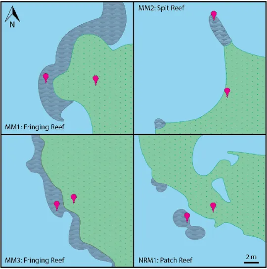
Figure 1: Oyster-reef morphologies and core locations………...5
Figure 2: Site map………7
Figure 3: 210Pb profiles with mass depth………13
Figure 4: MM1 with all models……….15
Figure 5: CRS model applied to all cores………..16
Figure 6: Mass accumulation rate comparison………..17
LIST OF ABBREVIATIONS CIC Constant Initial Concentration Model
CFCS Constant Flux Constant Sedimentation Model CRS Constant Rate of Supply Model
IPCC Intergovernmental Panel on Climate Change MAR Mass accumulation rate (g cm-2 yr-1)
MM Middle Marsh
NRM New River Marsh
210Pb
xs Excess 210Pb 210Pb
sup Supported 210Pb
INTRODUCTION
Salt-marshes and intertidal oyster-reefs are composed of important foundation species that provide similar benefits to coastal areas. They are habitats for coastal wildlife (Minello et al 1994, Shervette and Gelwick 2008, Johnson and Eggleston 2010, Scyphers et al 2011, Coen et al 2007, Tolley and Volety 2005), buffer shorelines from storms by attenuating wave energy (Knutson et al 1982, Koch et al 2009), reduce turbidity and provide water filtration (Christiansen et al 2000, Grizzle et al 2008), and have mechanisms to adapt to sea-level rise (Redfield 1965, DeLaune et al 1978, Allen and Rae 1988, Morris et al 2002, Rodriguez et al 2014, Ridge et al 2017). As sea-level and anthropogenic influence increased over the past 100 years, oyster-reefs have decreased in spatial extent by 64% and in biomass by 88% (zu Ermgassen et al 2012). Oyster-reefs commonly fringe the seaward edge of salt-marshes and, considering their shared roles, understanding how these two environments function in juxtaposition is important for improving restoration and conservation of these degraded habitats.
Oyster-reefs grow in succession, with new generations colonizing and building on top of previous generations (Graves 1901, Kennedy et al 1996). The morphology of intertidal oyster-reefs is based on water flow and survivorship of spat, with the long axis of a reef positioned perpendicular to mean flow and spat survivorship extending along this axis (Graves 1901). Common morphologies are patch reefs, fringing reefs, and fringing-spit reefs (Figure 1). Patch reefs are not directly connected to any other subaerial environments, yet they may be in
reefs grow along the perimeter of a salt-marsh, parallel to the marsh edge and fringing-spit reefs are elongated perpendicular to a marsh. These various morphologies may affect how the two environments interact as they adapt to sea-level rise.
A major process in oyster-reef and salt-marsh adaptation to sea-level rise is
results with moderate inundation increasing sediment accumulation but too much inundation causing marsh grasses to drown, resulting in erosion of the marsh.Salt-marsh and oyster-reef inundation is modulated by their elevation in relation to sea level. Sedimentation generally increases as sea-level rises (Kirwan 2010; Ridge et al., 2017), but these environments have a limit of sea-level rise because too much inundation will lead to drowning and erosion (Morris et al 2002, Reidenbach et al 2004). It is important to keep in mind the predicted increase in global sea-level over the next century (IPCC 2007) when studying these environments to understand how they will change and adapt with the conditions.
Salt-marsh sedimentation and adaptability to sea-level rise is widely studied on various timescales. However, less is known about intertidal oyster-reef sediment accumulation on multi-decadal timescales. Subtidal oyster-reefs and intertidal oyster-reefs have different sedimentation regimes because of the difference in inundation time. Subtidal reefs are always inundated, allowing full-time water filtration and capture of suspended sediments, while intertidal oyster-reefs are exposed to the atmosphere during low tide, limiting filtration and sediment capture (Bishop and Peterson 2005). So although DeAlteris (1988) studied subtidal oyster-reefs to
quantify biogenic sedimentation on reefs and to understand reef migration with sea-level rise, the conclusions are not necessarily applicable to intertidal oyster-reefs. Rodriguez et al (2014) studied intertidal reef growth on patch reefs over a 15-year period using Lidar and cores, concluding that oyster-reefs can vertically accrete faster than other coastal environments when faced with rising sea-levels. However, the study does not include other intertidal reef
morphologies, nor does it quantify sediment accumulation on a timescale that allows the
increases as sea-level increases, but these results were formed over a 5-year study. There is a clear lack of quantified sediment accumulation rates in intertidal oyster-reefs over a multi-decadal time period. Those data are especially lacking for oyster-reefs adjacent to salt-marshes, and to date there are no publications with such data.
When an oyster-reef is adjacent to a salt-marsh, its possible that the reef could affect sedimentation on the salt-marsh. The oyster-reef could act as a barrier and prevent sediments from reaching the marsh, similar to marsh levees described in Stumpf 1983. Rodriguez et al (2014) found that intertidal oyster-reefs in patch morphologies can outpace marsh sedimentation rates. If these results can be applied to oyster-reefs adjacent to marshes, it would allow the reef to act as a barrier, causing a high sediment accumulation rate on the oyster-reef compared to the marsh. Evidence in previous studies focusing on living shorelines shows that oyster-reefs promote sedimentation in adjacent salt-marshes (Swann 2008), so in another scenario the marsh could capture the majority of sediments from tidal inundation, starving the oyster-reef of
sediments, causing a higher sediment accumulation rate on the marsh compared to the oyster-reef. Lastly, because these two environments have similar mechanisms for sedimentation, when coupled adjacent to each other, they could have similar accumulation rates reflective of the controlling factors surrounding them including suspended sediment concentration in the water, tidal range, and storm frequency.
This study quantifies sediment accumulation rates on intertidal oyster-reefs of various morphologies and the adjacent marshes via 210Pb geochronology. It aims to determine the relationship of sedimentation between oyster-reef and marsh. These rates are quantified as sediment mass accumulation rates over an area (MAR; g cm-2 yr-1). The use of 210Pb
resolution. With this timescale we are able to measure sediment accumulation as compared to less permanent sediment deposition (McKee et al 1983), expressing the longer-term adaptation to sea-level rise. This is the first study to quantify sediment accumulation rates on such a time-scale for intertidal oyster-reefs, allowing a further understanding of reef dynamics.
STUDY SITE
Four natural marsh and oyster-reef sites outside Beaufort, North Carolina were chosen for this study (Figure 1 and 2, Table 1). Middle Marsh is located in Back Sound behind Shakleford Banks, and North River Marsh is in the North River Estuary, just north of Back Sound. These two environments, now comprised of modern salt-marsh, oyster-reefs, and sand flats, originated as flood-tide deltas that formed approximated 4000 to 2000 years ago (Berelson and Duncan Heron 1985). This area experiences a low and high tide twice daily with a mean tidal range of 0.95 m (NOAA Tides and Currents, Station ID 8656483, Beaufort, NC), andsalinities typically fall between 30 and 35 ppt. The salt-marsh and oyster-reefs used in this study are naturally formed and have undergone minimal anthropogenic change. In Middle Marsh site MM1 and MM3 have fringing reefs, and MM2 has a fringing-spit reef. In the North River Marsh, NRM1 has a patch reef that was once fringing the marsh and detached as the marsh transgressed upriver with sea-level rise (Ridge et al 2017). The core locations for each site are marked on Figure 1.
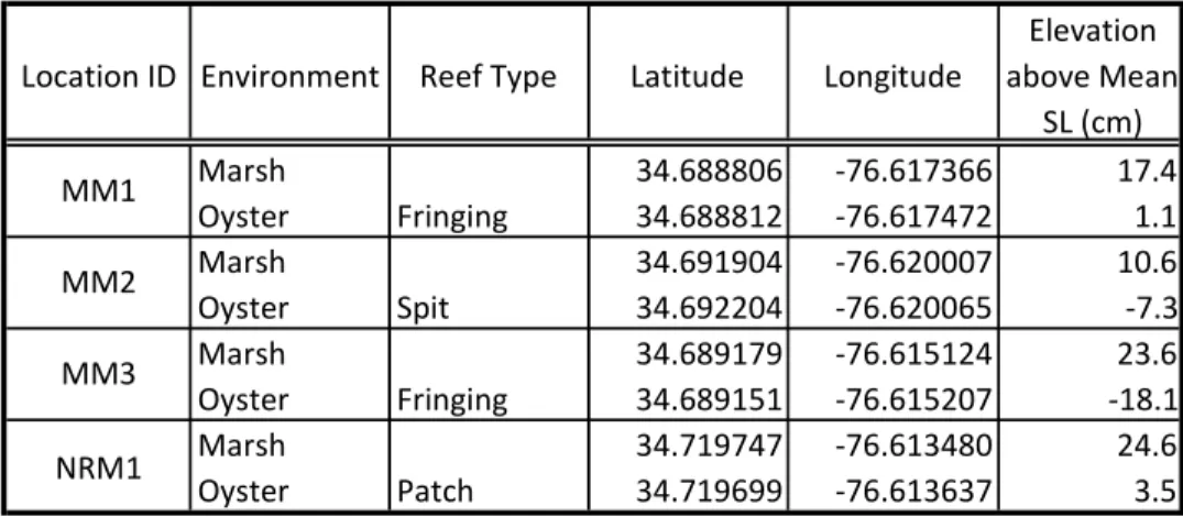
Table 1) Location and elevation of the top of each core used in this study
Location ID Environment Reef Type Latitude Longitude
Elevation above Mean
SL (cm)
Marsh 34.688806 -76.617366 17.4
Oyster Fringing 34.688812 -76.617472 1.1
Marsh 34.691904 -76.620007 10.6
Oyster Spit 34.692204 -76.620065 -7.3
Marsh 34.689179 -76.615124 23.6
Oyster Fringing 34.689151 -76.615207 -18.1
Marsh 34.719747 -76.613480 24.6
Oyster Patch 34.719699 -76.613637 3.5
MM1
MM2
MM3
METHODS
Core Collection
Oyster cores were collected between February and April of 2014. Marsh cores were collected in June 2015. At each marsh location, a core 1 m in length was extracted close to the marsh edge using a 10-cm diameter aluminum core tube. For the oyster-reefs, the same size core tube was pushed into the reef using a jackhammer. The cores were brought back to the lab and immediately sectioned. Marsh cores were sectioned into 1-cm intervals and, due to shell density, oyster cores were sectioned into 5-cm intervals. The oyster core subsections began below the living section of the oyster core, or the taphonomically active zone because the majority of sediment accumulation is below this point (Rodriguez et al 2014). The marsh sediments were freeze dried, and dry bulk density for each sample was calculated from the dry mass divided by the volume of the originally saturated sample. Half of each sample was dry-sieved using a 63 µm mesh sieve so those sediments could be used for 210Pb analysis. The oyster cores were wet sieved using a 2 mm sieve to separate sediment and shell, oven dried, and then half of each sample was dry-sieved (63µm). Dry bulk density for the oyster cores was calculated from one oyster core from a patch reef within the study area and applied to all the oyster cores.
210Pb Geochronology
210Pb is a naturally occurring radioisotope in the 238U decay series with a half-life of 22.3
years. With this short half-life, geochronology using 210Pb allows for high resolution sediment
that is produced in situ by the decay of its parent isotope 226Ra within the particle matrix. 210Pbsup
is in equilibrium with 226Ra and is generally consistent throughout the sediments of a given area. Excess 210Pb (210Pbxs) is the portion of 210Pb that is sorbed onto the particle from surrounding
waters and atmosphere. As sediments accumulate, buried sediments do not receive any additional
210Pb, and the buried excess 210Pb decays with time, eventually reaching 210Pb
sup levels. 210Pbsup
is calculated by determining the 210Pb concentration deep in the core where concentrations are constant. This stable concentration is the 210Pbsup. 210Pbxs in the depths above is calculated by
subtracting 210Pbsup from the total 210Pb concentration.
210Pb Analysis Via Alpha Spectrometry
The concentration of 210Pb (dpm g-1) in the sediments was determined through isotope-dilution alpha spectrometry of the granddaughter isotope, 210Po, which is in secular equilibrium with total 210Pb (El-Daoushy et al 1991, Flynn 1968, Matthews et al 2007). The fine fraction of each sample was spiked with 209Po tracer to determine chemical yield. The 209Po activity was determined using the certified natural reference standard IAEA-300. The vessels were
24 hours. Isotope concentration is reported in units of activity (dpm) per gram.
Modeling 210Pb Profiles
Down-core profiles of excess 210Pb concentration (dpm g-1) and dry bulk density (g cm-3) are used to establish geochronologies using various models. Since concentrations of 210Pb were
determined from the fine fraction of each sample, concentration values determined through α-particle spectrometry were normalize to the full sample. Sediment accumulation rates reported in cm yr-1 are often inflated because sediments at the top of a core are uncompacted compared to sediments down-core. To avoid issues with sediment compaction, mass depth down-core (g cm
-2), calculated from dry bulk density (g cm-3), is used in the models instead of depth down-core
(cm). This allows for the calculation of a mass accumulation rate (MAR, g cm-2 yr-1). The models here have been adapted from Appleby 2001 and Sanchez-Cabeza and Ruiz-Fernandez 2012. The three models used in this study are the Constant Initial Concentration (CIC), Constant Rate of Supply (CRS), and Constant Flux Constant Sedimentation (CFCS). Each of these 3 models has a set of assumptions that must be met. All the models were applied to each core, and the
assumptions were validated based on the profiles and the environmental information from each core location.
The CIC model utilizes the decay equation: Ci = C0 e-λt, where C0 is the initial
concentration, Ci is the concentration at an uncompacted depth i, λ is the decay constant of 210Pb
(0.03118), and t is the time elapsed since deposition. This model assumes that initial concentration, C0, is constant through depositional time, and is equal to 210Pb flux to the
The CRS model relies on total inventory of excess 210Pb down-core, reported in activity per unit volume (dpm cm-3), using the equation Ai = A0 e-λt.A0 is the total cumulative 210Pbxs
inventory within the core, calculated from the sum of the activity per unit volume (dpm cm-2) of each section in the core. Ai is the cumulative 210Pbxs inventory below section i (dpm cm-2), λ is
the decay constant, and t is the time elapsed since deposition. This model assumes that atmospheric flux is constant, so initial concentration and mass accumulation rate may vary inversely to one another.
The CFCS model may be applied as a piecewise model. It assumes that both flux and mass accumulation rate are constant in each piece of the model. It uses the equation ln(Ci) =
ln(C0)-(λ/r)*mi where the variables are the same as stated above, and mi is the dry mass of
RESULTS
210Pb Profiles
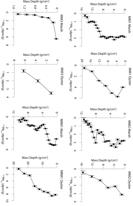
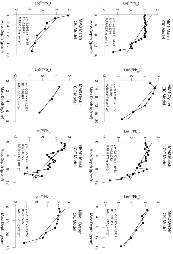
Figure 3 shows the 210Pbxs profiles with mass depth for each core. A table of values for
the profiles is in the Appendix, Table 1A. The 210Pb
xs profiles of most cores in this study do not
follow an exponential curve, which indicates variable accumulation rates down-core. All 8 cores were analyzed down core until 210Pbsup levels were reached, ensuring the full inventory of 210Pbxs
is accounted for. Table 2 shows the calculated flux of 210Pbxs (dpm cm-2 yr-1) in each core. Both
the marsh and oyster-reef at MM1 and MM2, and the marsh at NRM1 have flux values similar to the calculated North Carolina atmospheric flux, 0.83 ± 0.03 dpm cm-2 yr-1 (Graustein and
Turekian 1986, Benninger and Wells 1993). MM3 shows low values of flux, indicating extremely low sediment accumulation. The oyster core at NRM1 has a flux approximately 3 times the North Carolina average, which indicates high rates of sediment accumulation. The depth of measurable 210Pbxs varies in each core because of variable MARs and 210Pbxs flux at
each location. The final depth at each core is still within the marsh or oyster-reef environment as determined from root mass in marsh and shell material in oyster cores. All of the profiles show
210Pb
xs generally increasing up-core, indicating that these are non-erosive environments. The
oyster cores at each site have lower-resolution profiles due to the 5-cm core increments used in
Figure 3) Profiles of 210Pbxs with mass depth. The concentration of 210Pbxs generally increases
Table 2) Atmospheric flux and average MAR over the past 30 years for each location
Modeling 210Pb profiles
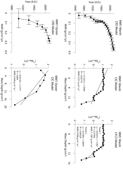
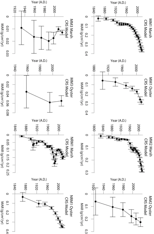
Figure 4 shows a graph of each model, CIC, CRS, and CFCS, applied to the marsh and oyster cores at MM1. In this figure the CIC models for MM1_Marsh and MM1_Oyster have an R2 value of 0.65 and 0.80, respectively. These low R2 values support the assumption that MAR may vary down core. The CFCS piecewise model does not apply to MM1_Oyster because there are not multiple distinct trends of sedimentation as is demonstrated in the CFCS piecewise model for MM1_Marsh. The CIC model graphs for the other sites are in Appendix 1. It is clear from the profiles that the CIC and CFCS model assumptions are not upheld, and that the CRS model is the best fit for the locations in this study. The CRS model allows each interval of the core to have a unique MAR, which creates a high-resolution profile of time versus MAR. Figure 5 shows the CRS model applied to all cores in this study. In each core, the average MAR over the last 30 years is similar to the MAR calculated using the CIC model, which lends validity to the results. The oyster cores in Figure 5 all have relatively high error compared to the marsh cores because of the larger sampling intervals in the oyster cores, but the oyster cores at sites MM1, MM2, and NRM1 show a general trend of increasing MAR toward the present, similar to the marsh cores at
Location ID Environment Reef Type
210Pb xsFlux
(dpm cm-2yr-1)
µ(Flux)
(dpm cm-2yr-1)
MAR 30-yr avg. (g cm-2yr-1)
µ(MAR) (g cm-2yr-1)
Marsh 1.04 0.02 0.260 0.049
Oyster Fringing 1.40 0.11 0.214 0.050
Marsh 0.81 0.02 0.199 0.036
Oyster Spit 0.68 0.11 0.187 0.097
Marsh 0.06 0.01 0.015 0.009
Oyster Fringing 0.29 0.05 0.049 0.042
Marsh 0.76 0.01 0.128 0.023
Oyster Patch 3.15 0.10 0.291 0.035
MM1
MM2
MM3
all sites. MM3_Oyster does not have an appreciable trend in MAR because 210Pbxs is only in the
top 15 cm. This indicates a very slow accumulation rate.
Figure 4) MM1_Marsh with the CRS, CIC, and CFCS model applied to it. MM1_Oyster with CRS and CIC. The graph of MM1_Oyster Ln(210Pbxs) v Mass Depth does not show more than
Figure 5) The CRS model applied to all 8 cores shows a general increase in MAR over time. Both marsh and oyster at MM1 and MM2 show similar trends of increasing MAR starting around the same time. Marsh and oyster at MM3 have MARs an order of magnitude lower than all other cores. The marsh and oyster at NRM1 do not share similar trends in sediment
Comparing MARs within sites
To compare the MARs of the marsh to the oyster-reef at each site, the average MAR over the last 30 years is used. Table 2 shows the average MAR of each core location and the
associated error. Figure 6 graphically displays this data with the oyster-reef MAR versus the salt-marsh MAR for each of the four sites, with a 1-to-1 line plotted for visual aid. Locations falling below the 1-to-1 line have a higher average salt-marsh MAR, while points above have a higher average oyster-reef MAR. MM1, MM2, and MM3 all fall on the 1-to-1 line within error. NRM1 is well above the 1-to-1 line, with the reef having a rate more than double of the associated marsh.
DISCUSSION
The use of the CRS model requires a full inventory to accurately model sediment accumulation because the model is a function of total inventory of 210Pbxs rather than initial
concentration. Since all cores were analyzed down-core until they reached 210Pb
sup levels, it can
be assumed that the total inventory is accounted for and the use of the CRS model is valid. Although the CIC model is not used for final analysis, the calculated MAR using the CIC model for each core is similar to the average MAR over the last 30 years using the CRS model, and that aids in validating the calculated MARs (see Appendix Figure 1A).
The general increasing MARs toward the present in all cores is expected because local sea-level rise has allowed salt-marshes and oyster-reefs to accumulate sediments at faster rates. Kemp et al (2011) determined that the average rate of sea-level rise in North Carolina since 1865 is 2.1 mm yr-1. This rate is based off the 210Pb geochronology of 2 marshes 40 and 155 km away from the Back Sound and North River Marsh area. The Beaufort, NC tide gauge shows local sea-level is rising at 3.04 ± 0.35 mm yr-1 based on data from 1953 to 2017 (NOAA Tides and
Currents, Station ID 8656483). The MARs calculated at each site, reported in g cm-2 yr-1, cannot be directly compared to local sea-level rise. However, the CRS model, validated with the CIC model, shows that these sites have existed as salt-marsh and oyster-reef during this rate of sea-level rise (oldest date between 1820 and 1840, MM2_Marsh), so the environments have kept up with sea-level rise of 2.1-3.04 mm yr-1. This gives a baseline for rates of local sea-level rise that
In comparing MARs of all the sites, both the marsh and fringing oyster-reef at site MM3 have a MAR one order of magnitude lower than the other sites. This low MAR is reflected in the low 210Pbxs flux (Table 2). Because of this low accumulation rate, only the top few sections of
each core had measurable 210Pb
xs, which created a very low-resolution profile and caused large
error in the CRS model. Although the oyster-reef at this site is calculated to have a MAR more than 3 times higher than the associated marsh, they both have extremely low MARs. This could be caused by many factors including marsh elevation above mean sea-level (23.6 cm) and oyster-reef elevation below mean sea-level (-18.1 cm), suspended sediment concentration, and
vegetation and oyster density. The higher marsh elevation may reduce sedimentation because it is above the optimal growth zone for this marsh, which causes limited inundation time and less sedimentation. The oyster-reef may be below its optimal growth zone, so the oysters are not able to filter suspended sediments as efficiently as the other oyster-reefs, which are all at a higher elevation. Regardless of why the sedimentation rates are low, it should be noted that the coupled marsh and fringing oyster-reef at MM3 both have very low MARs, indicating that they are experiencing similar sedimentation regimes.
Along with site MM3, site MM1 with a fringing oyster-reef and site MM2 with a
fringing-spit reef have similar MARs between the oyster-reef and adjacent marsh. The MARs at MM1 and MM2 overlap within error, yet all 3 pairings do vary in MAR. This can be attributed to varying environmental factors. It is possible that the close couplings at each site are due to
similar marsh grass and oyster densities, elevation in relation to one another, or site
past 30 years of sediment accumulation, living biomass density is probably not why these sites have similar MARs. Salt-marsh optimal growth zone is between mean sea-level and mean high water (Morris et al 2002), and oyster-reef optimal growth zone is between mean low water and mean sea-level (Ridge et al 2017). These are general zones, and will ultimately vary site to site, but the elevation difference between marsh and oyster-reef may be important in sediment
accumulation. However, the elevation of the marsh related to the oyster-reef changes at each site. Since each of these 3 sites show close coupling of marsh and reef, elevation difference is ruled out as the main cause for coupled MARs. Sedimentation regime has a stronger argument for oyster-reefs attached to an adjacent marsh experiencing a similar sediment accumulation rate as the marsh. When an intertidal oyster-reef is attached to a salt-marsh, the two environments experience similar tidal inundation, suspended sediment concentration, and storm frequency, so the environments have similar sediment deposition and accumulation over time.
Site NRM1 is the only site that does not show a close coupling of MAR between the oyster-reef and the marsh. Here, the oyster-reef is accumulating sediments at a rate that is just over double the rate of the marsh (0.291 ± 0.035 g cm-2 yr-1 and 0.128 ± 0.023 g cm-2 yr-1
respectively). The difference in 210Pbxs flux for this marsh and oyster-reef reflect the difference in
CONCLUSIONS
The CRS model applied to intertidal oyster-reefs show that these reefs experienced increased sediment accumulation as local sea-level increased over the past century. This indicates that with future sea-level rise of similar rates, intertidal oyster-reefs are capable of continuing to accumulate sediments and keep up with sea-level. With MARs an order of
magnitude lower than the other sites in this study, Site MM3 is an example showing that not all intertidal oyster-reefs are capable of accumulating sediments at high rates due to various factors including elevation, oyster density and suspended sediment concentration. However, the other sites show that intertidal oyster-reefs are capable of accumulating sediments as sea-level
increases if the other environmental conditions present are conducive to sediment accumulation. The coupling of intertidal oyster-reefs attached to marshes show a general trend of similar MARs. The large difference between the oyster-reef and salt-marsh MARs at site NRM1 point toward possible interference of sedimentation due to the patch reef. Conclusive results about patch reefs affecting marsh MARs cannot be determined in this study and should be studied further to understand the relationship of sedimentation between patch reefs and near-by salt-marsh.
APPENDIX
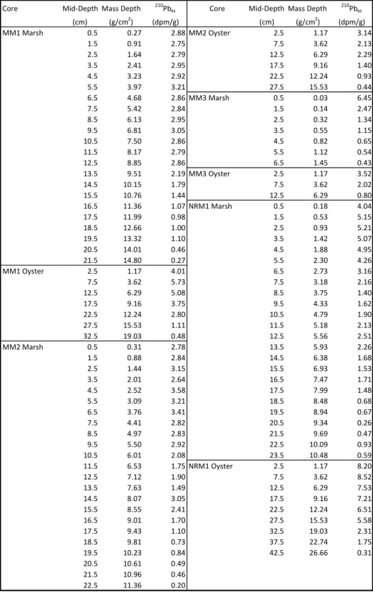
Table 1A) 210Pbxs (dpm g-1)concentrations per core with depth (cm) and mass depth (g cm-2). All
cores reached constant 210Pbsup concentration at approximately 1 dpm g-1, and total inventory is
accounted for within each core.
Core Mid-Depth Mass Depth 210Pbxs Core Mid-Depth Mass Depth 210Pbxs
(cm) (g/cm2) (dpm/g) (cm) (g/cm2) (dpm/g)
MM1 Marsh 0.5 0.27 2.88 MM2 Oyster 2.5 1.17 3.14
1.5 0.91 2.75 7.5 3.62 2.13
2.5 1.64 2.79 12.5 6.29 2.29
3.5 2.41 2.95 17.5 9.16 1.40
4.5 3.23 2.92 22.5 12.24 0.93
5.5 3.97 3.21 27.5 15.53 0.44
6.5 4.68 2.86 MM3 Marsh 0.5 0.03 6.45
7.5 5.42 2.84 1.5 0.14 2.47
8.5 6.13 2.95 2.5 0.32 1.34
9.5 6.81 3.05 3.5 0.55 1.15
10.5 7.50 2.86 4.5 0.82 0.65
11.5 8.17 2.79 5.5 1.12 0.54
12.5 8.85 2.86 6.5 1.45 0.43
13.5 9.51 2.19 MM3 Oyster 2.5 1.17 3.52
14.5 10.15 1.79 7.5 3.62 2.02
15.5 10.76 1.44 12.5 6.29 0.80
16.5 11.36 1.07 NRM1 Marsh 0.5 0.18 4.04
17.5 11.99 0.98 1.5 0.53 5.15
18.5 12.66 1.00 2.5 0.93 5.21
19.5 13.32 1.10 3.5 1.42 5.07
20.5 14.01 0.46 4.5 1.88 4.95
21.5 14.80 0.27 5.5 2.30 4.26
MM1 Oyster 2.5 1.17 4.01 6.5 2.73 3.16
7.5 3.62 5.73 7.5 3.18 2.16
12.5 6.29 5.08 8.5 3.75 1.40
17.5 9.16 3.75 9.5 4.33 1.62
22.5 12.24 2.80 10.5 4.79 1.90
27.5 15.53 1.11 11.5 5.18 2.13
32.5 19.03 0.48 12.5 5.56 2.51
MM2 Marsh 0.5 0.31 2.78 13.5 5.93 2.26
1.5 0.88 2.84 14.5 6.38 1.68
2.5 1.44 3.15 15.5 6.93 1.53
3.5 2.01 2.64 16.5 7.47 1.71
4.5 2.52 3.58 17.5 7.99 1.48
5.5 3.09 3.21 18.5 8.48 0.68
6.5 3.76 3.41 19.5 8.94 0.67
7.5 4.41 2.82 20.5 9.34 0.26
8.5 4.97 2.83 21.5 9.69 0.47
9.5 5.50 2.92 22.5 10.09 0.93
10.5 6.01 2.08 23.5 10.48 0.59
11.5 6.53 1.75 NRM1 Oyster 2.5 1.17 8.20
12.5 7.12 1.90 7.5 3.62 8.52
13.5 7.63 1.49 12.5 6.29 7.53
14.5 8.07 3.05 17.5 9.16 7.21
15.5 8.55 2.41 22.5 12.24 6.51
16.5 9.01 1.70 27.5 15.53 5.58
17.5 9.43 1.10 32.5 19.03 2.31
18.5 9.81 0.73 37.5 22.74 1.75
19.5 10.23 0.84 42.5 26.66 0.31
20.5 10.61 0.49
21.5 10.96 0.46
WORKS CITED
Allen, J. R. L., & Rae, J. E. (1988). Vertical salt-marsh accretion since the Roman Period in the Severn Estuary, southwest Britain. Marine Geology, 83(1-4), 225–235.
Appleby, P. G. (2001). Chronostratigraphic Techniques in Recent Sediments. Tracking Environmental Change Using Lake Sediments, 1, 1–33.
Benninger, L. K., & Wells, J. T. (1993). Sources of sediment to the Neuse River estuary, North Carolina. Marine Chemistry, 43(1-4), 137–156.
Berelson, W. M., & Heron, S. D. (1985). Correlations between Holocene flood tidal delta and barrier island inlet fill sequences: Back Sound‐Shackleford Banks, North Carolina.
Sedimentology, 32(2), 215–222.
Bishop, M. J., & Peterson, C. H. (2005). Direct effects of physical stress can be counteracted by indirect benefits: oyster growth on a tidal elevation gradient. Oecologia, 147(3), 426–433. Blanchard, R. L. (1966). Rapid Determination of Lead-210 and Polonium-210 in Environmental
Samples by Deposition on Nickel. Analytical Chemistry, 38(2), 189–192.
Christiansen, T., Wiberg, P. L., & Milligan, T. G. (2000). Flow and Sediment Transport on a Tidal Salt Marsh Surface. Estuarine, Coastal and Shelf Science, 50(3), 315–331.
Coen, L. D., Brumbaugh, R. D., Bushek, D., Grizzle, R., Luckenbach, M. W., Posey, M. H., et al. (2007). Ecosystem services related to oyster restoration. Marine Ecology Progress Series,
341, 303–307.
DeAlteris, J. T. (1988). The Geomorphic Development of Wreck Shoal, a Subtidal Oyster Reef of the James River, Virginia. Estuaries, 11(4), 240.
Delaune, R. D., Patrick, W. H., & Buresh, R. J. (1978). Sedimentation rates determined by 137Cs dating in a rapidly accreting salt marsh. Nature, 275(5680), 532–533.
El-Daoushy, F., Olsson, K., & Garcia-Tenorio, R. (1991). Accuracies in Po-210 determination for lead-210 dating. Hydrobiologia, 214(1), 43–52.
Flynn, W. W. (1968). The determination of low levels of polonium-210 in environmental materials. Analytica Chimica Acta, 43, 221–227.
Graustein, W. C., & Turekian, K. K. (1986). 210Pb and 137Cs in air and soils measure the rate and vertical profile of aerosol scavenging. Journal of Geophysical Research: Atmospheres,
91(D13), 14355–14366.
Grizzle, R. E., Greene, J. K., & Coen, L. D. (2008). Seston Removal by Natural and Constructed Intertidal Eastern Oyster (Crassostrea virginica) Reefs: A Comparison with Previous
Laboratory Studies, and the Value of in situ Methods. Estuaries and Coasts, 31(6), 1208– 1220.
Johnson, E. G., & Eggleston, D. B. (2010). Population density, survival and movement of blue crabs in estuarine salt marsh nurseries. Marine Ecology Progress Series, 407, 135–147. Kennedy, V., White, M. E., & Wilson, E. A. (1996). The Eastern Oyster: Crassostrea viginica.
Maryland Sea Grant College, 734.
Kirwan, M. L., Guntenspergen, G. R., D'Alpaos, A., Morris, J. T., Mudd, S. M., & Temmerman, S. (2010). Limits on the adaptability of coastal marshes to rising sea level. Geophysical Research Letters, 37(23).
Knutson, P. L., Brochu, R. A., Seelig, W. N., & Inskeep, M. (1982). Wave damping in Spartina alterniflora marshes. Wetlands, 2(1), 87–104.
Koch, E. W., Barbier, E. B., Silliman, B. R., Reed, D. J., Perillo, G. M., Hacker, S. D., et al. (2009). Non-linearity in ecosystem services: temporal and spatial variability in coastal protection. Frontiers in Ecology and the Environment, 7(1), 29–37.
Martin, P., & Hancock, G. (1992). Routine analysis of naturally occurring radionuclides in environmental samples by alpha-particle spectrometry. International Nuclear Information System.
Matthews, K. M., Kim, C.-K., & Martin, P. (2007). Determination of 210Po in environmental materials: A review of analytical methodology. Applied Radiation and Isotopes, 65(3), 267– 279.
McKee, B. A., Nittrouer, C. A., & DeMaster, D. J. (1983). Concepts of sediment deposition and accumulation applied to the continental shelf near the mouth of the Yangtze River. Geology,
11(11), 631.
Minello, T. J., Zimmerman, R. J., & Medina, R. (1994). The importance of edge for natant macrofauna in a created salt marsh. Wetlands, 14(3), 184–198.
Morris, J. T., Sundareshwar, P. V., Nietch, C. T., Kjerfve, B., & Cahoon, D. R. (2002). Responses of coastal wetlands to rising sea level. Ecology, 83(10), 2869–2877.
Neumeier, U., & Ciavola, P. (2004). Flow Resistance and Associated Sedimentary Proce in a Spartina maritima Salt-Marsh. Journal of Coastal Research, 20(2), 435–447.
Redfield, A. C. (1965). Ontogeny of a Salt Marsh Estuary. Science, 147(3653), 50–55. Reidenbach, M. A., Berg, P., Hume, A., Hansen, J. C. R., & Whitman, E. (2013).
Hydrodynamics of intertidal oyster reefs: The influence of boundary layer flow processes on sediment and oxygen exchange. Limnology and Oceanography, 3, 225–239.
Ridge, J. T., Rodriguez, A. B., & Fodrie, F. J. (2017). Salt Marsh and Fringing Oyster Reef Transgression in a Shallow Temperate Estuary: Implications for Restoration, Conservation and Blue Carbon. Estuaries and Coasts, 40(4), 1–15.
Ridge, J. T., Rodriguez, A. B., Joel Fodrie, F., Lindquist, N. L., Brodeur, M. C., Coleman, S. E., et al. (2015). Maximizing oyster-reef growth supports green infrastructure with accelerating sea-level rise. Scientific Reports, 5, 14785.
Rodriguez, A. B., Fodrie, F. J., Ridge, J. T., Lindquist, N. L., Theuerkauf, E. J., Coleman, S. E., et al. (2014). Oyster reefs can outpace sea-level rise. Nature Climate Change, 4(6), 493–497. Sanchez-Cabeza, J. A., & Ruiz-Fernández, A. C. (2012). 210Pb sediment radiochronology: An
integrated formulation and classification of dating models. Geochimica Et Cosmochimica Acta, 82(C), 183–200.
Sanchez-Cabeza, J. A., Masqué, P., & Ani-Ragolta, I. (1998). 210Pb and210Po analysis in sediments and soils by microwave acid digestion. Journal of Radioanalytical and Nuclear Chemistry, 227(1-2), 19–22.
Scyphers, S. B., Powers, S. P., Heck, K. L., & Byron, D. (2011). Oyster Reefs as Natural Breakwaters Mitigate Shoreline Loss and Facilitate Fisheries. PLoS ONE, 6(8), e22396. Shervette, V. R., & Gelwick, F. (2008). Relative nursery function of oyster, vegetated marsh edge, and nonvegetated bottom habitats for juvenile white shrimp Litopenaeus setiferus.
Wetlands Ecology and Management, 16(5), 405–419.
Stumpf, R. P. (1983). The process of sedimentation on the surface of a salt marsh. Estuarine, Coastal and Shelf Science, 17, 495–508.
Swann, L. (2008). The use of living shorelines to mitigate the effects of storm events on Dauphin Island, Alabama, USA. American Fisheries Society Symposium.
Zu Ermgassen, P. S. E., Spalding, M. D., Blake, B., Coen, L. D., Dumbauld, B., Geiger, S., et al. (2012). Historical ecology with real numbers: past and present extent and biomass of an imperiled estuarine habitat. Proceedings of the Royal Society B: Biological Sciences,