A continuum mechanics-based
musculo-mechanical model for esophageal
transport
Wenjun Kou
Theoretical and Applied Mechanics, Northwestern University, 2145 Sheridan Road, Evanston, Illinois 60208, USA
Boyce E. Griffith
Departments of Mathematics and Biomedical Engineering, University of North Carolina at Chapel Hill, Phillips Hall, Campus Box 3250, Chapel Hill, North
Carolina 27599-3250, USA
John E. Pandolfino
Department of Medicine, Feinberg School of Medicine, Northwestern University, 676 North Saint Clair Street, 14th Floor, Chicago, Illinois 60611, USA
Peter J. Kahrilas
Department of Medicine, Feinberg School of Medicine, Northwestern University, 676 North Saint Clair Street, 14th Floor, Chicago, Illinois 60611, USA
Neelesh A. Patankar
∗
Department of Mechanical Engineering, Northwestern University, 2145 Sheridan Road, Evanston, Illinois 60208, USA
Abstract
In this work, we extend our previous esophageal transport model using an immersed boundary (IB) method with discrete fiber-based structural model, to one using a continuum mechanics-based model that is approximated based on finite elements (IB-FE). To deal with the leakage of flow when the Lagrangian mesh becomes coarser than the fluid mesh, we employ adaptive interaction quadrature points to deal with Lagrangian-Eulerian interaction equations based on a previous work (Griffith and Luo [1]). In particular, we introduce a new anisotropic adaptive interaction quadra-ture rule. The new rule permits us to vary the interaction quadraquadra-ture points not only at each time-step and element but also at different orientations per element. This helps to avoid the leakage issue without sacrificing the computational efficiency
and accuracy in dealing with the interaction equations. For the material model, we extend our previous fiber-based model to a continuum-based model. We present for-mulations for general fiber-reinforced material models in the IB-FE framework. The new material model can handle non-linear elasticity and fiber-matrix interactions, and thus permits us to consider more realistic material behavior of biological tissues. To validate our method, we first study a case in which a three-dimensional short tube is dilated. Results on the pressure-displacement relationship and the stress dis-tribution matches very well with those obtained from the implicit FE method. We remark that in our IB-FE case, the three-dimensional tube undergoes a very large deformation and the Lagrangian size becomes about 6 times of Eulerian mesh-size in the circumferential orientation. To validate the performance of the method in handling fiber-matrix material models, we perform a second study on dilating a long fiber-reinforced tube. Errors are small when we compare numerical solutions with analytical solutions. The technique is then applied to the problem of esophageal transport. We use two fiber-reinforced models for the esophageal tissue: a bi-linear model and an exponential model. We present three cases on esophageal transport that differ in the material model and the muscle fiber architecture. The overall transport features are consistent with those observed from the previous model. We remark that the continuum-based model can handle more realistic and complicated material behavior. This is demonstrated in our third case where a spatially varying fiber architecture is included based on experimental study. We find that this unique muscle fiber architecture could generate a so-called pressure transition zone, which is a luminal pressure pattern that is of clinical interest. This suggests an important role of muscle fiber architecture in esophageal transport.
Key words: fluid-structure interaction, immersed boundary method, esophageal transport, fiber-reinforced model
1 Introduction
The immersed boundary (IB) method was introduced to model blood flow through heart valves [2], and has been widely used to simulate biological fluid dynamics [3,4,5,6,7]. The IB method has also been extended to deal with appli-cations involving kinematic constraints [5], the electric field [8,9] and thermal fluctuations [10], among others. The IB method utilizes a Eulerian descrip-tion of the momentum and continuity equadescrip-tions of the fluid-structure system, and a Lagrangian description of the displacements and stresses/forces of the structure (i.e. the solid). Thus it permits nonconforming discretizations of the fluid and the structure, and allows the Lagrangian mesh to move freely over the background Eulerian mesh. This approach does not require a body-fitted
∗ Corresponding author.
fluid mesh. Variables on the two meshes communicate via integral transforms with delta function kernels. In the conventional IB method [11], the Eule-rian fluid flow is described on a regular Cartesian grid and the Lagrangian structure in the discretized form is modeled by families of elastic fibers that can generate stretching and bending forces. This material model is referred to here as the fiber-based material model. The Lagrangian-Eulerian interaction equations are utilized to spread elastic forces from the Lagrangian nodes to the Eulerian (i.e. fluid) grid and interpolate the Eulerian fluid velocity to the Lagrangian nodes. This conventional IB method is referred to as the IB-fiber
method. The IB-fiber method is convenient to use in practice due to its simplic-ity in describing the elastic force. However, it also presents some challenges. First, the capability to model more realistic complex material behaviors is limited. The IB-fiber method uses a structure-based model (i.e. using beams, springs etc.); not a continuum-based model. Thus, it is difficult to incorporate a continuum-based description of material’s elasticity that is used for many biological tissues. Second, there is the issue of fluid leaking through the im-mersed structure. The IB-fiber model uses Lagrangian nodes to interact with the fluid grid. The Lagrangian mesh size defined by neighboring Lagrangian nodes vary spatially and temporally as those nodes will move according to the dynamics. Leakage can occur if the Lagrangian mesh becomes much coarser than the Eulerian mesh [11]. Recently, Griffith and Luo [1] introduced a ver-sion of the IB method that uses a finite element (FE) method to describe the elastic model. This method also allows interaction equations to be handled dif-ferently, such that the Lagrangian mesh can be coarser than the Eulerian grid without leakage. This new method here is referred to as the IB-FE method. Here we extend our previous IB-fiber based esophageal transport model to a IB-FE based esophageal transport model.
Esophageal transport is a bio-physical process that transfers food bolus from the pharynx to the stomach through a tube-like esophagus [12]. It involves interactions between a liquid-like bolus, the esophageal wall, and neurally controlled muscle activation. The esophageal wall consists of mucosal, circular muscle, and longitudinal muscle layers. The muscle activation involves the acti-vation of muscle fibers in, both, circular and longitudinal muscle layers [13,14].
we extend our fiber-based material model to fiber-reinforced continuum-based material model. We present a generic mathematical formulation to incorporate such fiber-reinforced material models into the IB-FE framework.
Esophageal transport problem is a numerically challenging problem. It in-volves multiple-length scales, from 0.3 mm to around 200 mm. It also inin-volves very large deformations, which result from interactions among the fluid, struc-ture, and muscle activation. As a result, leakage is a challenging issue. Our strategy in the previous IB-fiber-based model was to use a fine Lagrangian mesh in the inner-most layers, such that the Lagrangian mesh is always finer than the fluid mesh even under the largest dilation. However, such an ap-proach requires to know the deformation level during the whole dynamics in advance. This may not be practical in many cases. It also adds to the compu-tational cost. Here, we introduce a new approach to tackle the leakage issue following the work by Griffith and Luo [1]. Specifically, Griffith and Luo [1] introduced an adaptive interaction quadrature rule to deal with interaction equations. Their adaptive interaction quadrature rule could vary time-step by time-step, element by element to avoid the leakage issue. But it could lead to a unnecessarily large number of interaction quadrature points and impact the computational efficiency in certain cases. In this work, we extend the previ-ous adaptive interaction quadrature rule [1], referred to here as the isotropic adaptive interaction quadrature rule, to a so-called anisotropic adaptive inter-action quadrature rule. The anisotropic adaptive interaction quadrature rule is able to handle the variation of the aspect ratio of Lagrangian elements, and permits us to vary interaction quadrature points orientation by orientation per element. Therefore, it not only helps to avoid the leakage issue even when the Lagrangian mesh becomes much coarser than the Eulerian mesh, it also reduces the number of interaction quadrature points at each time step. This is especially useful when a non-uniform Eulerian mesh is used or the Lagrangian structure undergoes a very large deformation. For our large-scale esophageal transport model presented here, cases using the anisotropic adaptive inter-action quadrature rule run about twice faster than cases using the previous isotropic adaptive interaction quadrature rule.
2 Mathematical formulation
2.1 The immersed boundary method
The IB-FE method [6] employs an Eulerian description for the momentum equation and continuity equation, and a Lagrangian description for the de-formation of the immersed structure and the resulting structural forces. Let
x = (x1, x2, ...) ∈ Ω denote fixed Cartesian coordinates. Ω ⊂ Rd, d = 2 or 3,
denotes the fixed domain occupied by the entire fluid-structure system. We use s = (s1, s2, ...) ∈U to denote the Lagrangian coordinates attached to the
immersed structure, whereU denotes the Lagrangian domain in the reference configuration. We letχ(s, t)∈Ω denote the physical position of material point
sat timet. We denote the physical region occupied by the structure and fluid at timet as Ωs(t) =χ(U, t)⊆Ω and Ωf(t) = Ω\Ωs(t), respectively. Since we
consider here that the structure is immersed in the fluid, the fluid-structure interface can be denoted as ∂Ωs(t). The boundary of the whole domain, Ω is
denoted as ∂Ω. Then, the governing equations in the fluid domain, Ωf(t) are,
ρf ∂u f
∂t (x, t) +u
f(x, t)· ∇uf(x, t)
!
− ∇ ·σf = 0, (1)
∇ ·uf(x, t) =qf(x, t), (2)
whereρf,ufis the fluid density and velocity, andσf is the fluid stress.qf(x, t) is the fluid source, whose temporal-spatial distribution and strength is assumed to be known. qf(x, t) is non-zero only in the fluid domain.
We consider the structure is incompressible. Thus, governing equations in the structure domain, Ωs(t) are
ρs ∂u s
∂t (x, t) +u
s(x, t)· ∇us(x, t)
!
− ∇ ·σs = 0, (3)
∇ ·us(x, t) = 0. (4)
The interface conditions on the fluid-structure interface, ∂Ωs(t) are
σf·n=σs·n, (5)
uf =us, (6)
wherenis the outward normal unit vector to∂Ωs(t), outward being away from
On the boundary of the entire domain, ∂Ω
uf=uf∂Ω, (7)
whereuf∂Ω is the specified velocity on the boundary,∂Ω. Eq. (7) considers the Dirichlet boundary conditions, but the formulation can be easily extended to consider other boundary conditions. Notice that since we consider the struc-ture is immersed in the fluid, ∂Ω is the boundary of the fluid domain only. Eq. (7) stays unchanged in the IB formulation, and thus omitted during our following discussions in this section.
The governing equations above can be recast into an alternate form that is appropriate for IB implementation. A derivation of the IB governing equations using the principle of virtual work using a weak form has been provided by Boffi et al. [22]. In Appendix A we provide an alternate derivation based on the strong form that is pedagogically useful.
In our current work, we consider that the fluid-structure system possesses a uniform mass density ρ, i.e.ρs =ρf =ρ, and a uniform dynamic viscosity µ. This simplification implies that the immersed structure is neutrally buoyant and viscoelastic rather than purely elastic. Then the resulting IB governing equations can be written as below,
ρ ∂u
∂t(x, t) +u(x, t)· ∇u(x, t)
!
=−∇p(x, t) +µ∇2u(x, t) +fe, (8)
∇ ·u(x, t) =q(x, t), (9)
fe = Z
Ωs(t)∇ ·σ
eδ(x−χ(s, t))dχ(s, t)
−
Z
∂Ωs(t)σ
e·nδ(x−χ(s, t))da(χ(s, t)),
(10)
σe =F[χ(·, t)], (11)
where q(x, t) is a given fluid source, such that q(x, t)|Ωf(t) = qf(x, t), and
q(x, t)|Ωs(t)= 0.σeis the elastic stress of the immersed structure in the current configuration, i.e. the Cauchy elastic stress. fe is the Eulerian force density.
δ(x) is thed-dimensional delta function. Eq. (11) is the elastic stress equation that depends on the material model of the structure.
P is defined such that
Z
∂V P
e·NdA(s) = Z ∂χ(V,t)
σe·nda(x), (12)
for any smooth region V ⊂ U. N and n are the outward unit normal along
∂V and χ(V, t), respectively. Based on the divergence theorem, eq. (12) also implies,
Z
V
∇ ·Peds=Z
χ(V,t)
∇ ·σedx. (13)
Substituting eqs. (12) and (13) into eq. (10), we obtain
fe= Z
U
∇s·Peδ(x−χ(s, t))ds
−
Z
∂UP
e·Nδ(x−χ(s, t))dA(s), (14)
where∇s·Peis referred to as theLagrangian internal force density, andPe·N
is referred to as theLagrangian transmission force density. Like in the previous work [1], we introduce the Lagrangian force density, denoted asFe, as follows
fe= Z
U
Fe(s, t)δ(x−χ(s, t))ds. (15)
Feneeds to include both the internal and transmission force density. This can be done by employing the weak form as below,
Z
U
Fe(s, t)·V(s)ds= Z
U
(∇s·Pe)·V(s)ds−
Z
∂UP e·
N·V(s)dA(s)
=−
Z
UP
e: ∇
sV(s)ds, (16)
for any Lagrangian test function V(s) defined on U.
Based on eqs. (15)-(16), we obtain
ρ ∂u
∂t +u· ∇u
!
=−∇p+µ∇2u+fe, (17)
∇ ·u =q, (18)
fe(x, t) = Z
U
Fe(s, t)δ(x−χ(s, t))ds, (19)
Z
U
Fe(s, t)·V(s)ds=−
Z
UP
e: ∇
sV(s)ds,∀V(s), (20)
∂χ
∂t(s, t) =
Z
Ω
u(x, t)δ(x−χ(s, t))dx, (21)
where fe(x, t) and Fe(s, t) are the Eulerian and Lagrangian elastic force den-sities. Eq. (21) is the velocity-interpolating equation, which determines the velocity field on the Lagrangian system based on the Eulerian velocity field. Eq. (22) is the elastic stress equation that computesPe based on the material model of the structure.
Notice that eq. (20) is also a projection, which projects the Lagrangian force densityFe(s, t) into the function space defined by V(s). Thus, we introduce a similar projection on the Lagrangian velocity field. This is done as below,
Ue(s, t) = Z
Ω
u(x, t)δ(x−χ)dx, (23)
Z
U ∂χ
∂t(s, t)·V(s)ds=
Z
U
Ue(s, t)·V(s)ds,∀V(s), (24)
where Ue(s, t) is an intermediate Lagrangian velocity field. The final La-grangian velocity field ∂χ∂t(s, t) is a projection of the intermediate Lagrangian velocity field into the function space defined byV(s). Consequently, we obtain a new set of equations as below,
ρ ∂u
∂t +u· ∇u
!
=−∇p+µ∇2u+fe, (25)
∇ ·u=q, (26)
fe(x, t) = Z
U
Fe(s, t)δ(x−χ(s, t))ds, (27)
Z
U
Fe(s, t)·V(s)ds=−
Z
UP
e
: ∇sV(s)ds,∀V(s), (28)
Ue(s, t) = Z
Ω
u(x, t)δ(x−χ)dx, (29)
Z
U ∂χ
∂t(s, t)·V(s)ds=
Z
U
Ue(s, t)·V(s)ds,∀V(s), (30)
Pe=G[χ(·, t)]. (31)
We use eqs. (25) - (31) in the current work.
The above formulation differs from that of the IB-fiber method mainly in two parts: the treatment of the Lagrangian-Eulerian interactions and the descrip-tion of material elasticity. We proceed by briefly discussing these two parts, respectively. We refer to the prior work [1] for details on other aspects, includ-ing the spatial discretization, temporal discretization, and implementation.
2.2 Lagrangian-Eulerian Interactions
Eqs. (27) - (30) are equations on the Lagrangian-Eulerian interactions. Since those equations involve the weak form, we first introduce FE-based Lagrangian discretization. Let Th = ∪eUe be a triangulation of U composed of elements Ue, and {φl(s)}Ml=1 denote the Lagrangian basis functions. Then the physical
configuration of the Lagrangian structure,χ(s, t) is approximated by
χh(s, t) =
M
X
l=1
χl(t)φl(s), (32)
whereχl(t) is the time-dependent physical position of the Lagrangian nodesl.
To satisfy the discretized power identity, we also approximate the Lagrangian force density F(s, t) using the same shape functions as below
Fh(s, t) = M
X
l=1
Fl(t)φl(s), (33)
where Fl(t) is the nodal value of the Lagrangian force density. If we restrict
the test functions to be linear combinations of the Lagrangian basis function, then we can obtain semi-discretized equations on the Lagrangian-Eulerian interactions as below
f(x, t) =X
e
Z
Ue
F(s, t)δ(x−χ(s, t))ds
=X e X l Z Ue
φl(s)δ(x−χ(s, t))ds
Fl(t),
(34) X e X l Z Ue
φl(s)φm(s)ds
Fl(t) =−
X
e
Z
Ue
P· ∇sφm(s)ds, (35)
U(s, t) = Z
Ω
u(x, t)δ(x−χ(s, t))dx, (36)
X e X l Z Ue
φl(s)φm(s)ds
∂χ
l ∂t (t) =
X
e
Z
Ue
U(s, t)φm(s)ds. (37)
Notice that the above equations involve five integrals over the Lagrangian do-main. We remark that we use two different quadrature rules in approximating these five integrals, for reasons that will be discussed later. Specifically, we refer to the first quadrature rule as theinteraction quadrature rule, and apply it to the right-hand integrals in eqs. (34) and (37); we refer to the second quadrature rule as the elasticity quadrature rule and apply it to eq. (35) and the left-hand integral in eq. (37). More clearly, we let Iqp andωIqpdenote the
weights in each element. Then eqs. (34) -(37) can be written as,
f(x, t) =X
e
X
Iqp∈Ue
X
l
φl(sIqp)ωIqpδ(x−χ(sIqp, t))Fl(t), (38)
X
e
X
Eqp∈Ue
X
l
φl(sEqp)φm(sEqp)ωEqpFl(t) =−
X
e
X
Eqp∈Ue
PEqp· ∇sφm(sEqp)ωEqp,
(39)
U(sIqp, t) =
Z
Ω
u(x, t)δ(x−χ(sIqp, t))dx,
(40)
X
e
X
Eqp∈Ue
X
l
φl(sEqp)φm(sEqp)ωEqp ∂χl
∂t (t) =
X
e
X
Iqp∈Ue
U(sIqp, t)φm(sIqp)ωIqp.
(41)
The reason we have a separate quadrature rule in dealing with Lagrangian-Eulerian interactions is because the interaction quadrature rule is associated with (at least) three issues. First, the distribution of quadrature points relates to the leakage issue. In the conventional IB method, fluid leakage occurs when the Lagrangian mesh is coarser than the fluid mesh. Unlike the conventional IB method, the current IB-FE method employsinteraction quadrature points, instead of the Lagrangian nodes, to spread the Lagrangian forcing to, and interpolate the velocity from, the Eulerian field. This can be seen from eqs. (38) and (40). Thus, to avoid the leakage, we only need to ensure that the “submesh” composed of the interaction quadrature points is not coarser than the fluid mesh. To address the temporal-spatial variation of the Lagrangian mesh size during the interaction, we only need to vary the distribution of quadrature points. Second, the choice of the quadrature rule relates to the ac-curacy of the approximation. Unlike eq. (39), the integrand of the right-hand integral of eq. (38) contains a non-rational function, i.e. the delta function. Traditional quadrature rules that are optimal for polynomial integrand may not be optimal in eq. (38). Third, the number of quadrature points relates to the computational cost. Notice that adding one more interaction quadrature point will bring (at least) two more evaluations of the non-rational delta func-tion at each time-step. Thus, for three-dimensional large-scale simulafunc-tions, a large number of the interaction quadrature points per element could greatly impact the computational efficiency.
2.2.1 Anisotropic adaptive interaction quadrature rule
We restrict our finite elements as bi-linear finite elements (i.e. four-node quadri-lateral elements) in two dimensions and tri-linear elements (i.e eight-node hexahedral elements) in three dimensions. We discuss our treatment in three-dimensional cases as an example.
Consider an arbitrary eight-node hexahedral element, e. In the reference con-figuration, it has three orientations, denoted as (ˆsi(e), i = 1, ..,3) and four
edges along each orientation, denoted as (dsˆa
i(e), i= 1, ..,3;a= 1, ..,4). In the
current configuration, the four edges of the element e along each orientation become (dˆla
i(e, t), i = 1, ..,3;a = 1, ..,4). Based on the mapping χ(s, t), we
can compute the maximum length of the four edges along each orientation, denoted by (dˆlmaxi (e, t), i= 1, ..,3).
Our fluid grid is a Cartesian grid. If the finest fluid grid size is uniform, i.e.
hx =hy = hz =h, then we compute mesh-size ratios along each orientation,
denoted as (ri(e, t), i= 1, ..,3),
ri(e, t) =
dˆlimax(e, t)
h (i= 1, ..,3). (42)
Notice that if the finest fluid grid size is non-uniform, one can compute
h= min(hx, hy, hz), and then compute (ri(e, t), i= 1, ..,3) based on eq. (42).
However, another formulation can be obtained if we know in advance the align-ment information of the edges, (dˆla
i(e, t), i= 1, ..,3;a = 1, ..,4). For example,
in our esophageal model, the structure is a three-dimensional long tube de-scribed by the cylindrical coordinate system s = (R,Θ, Z). Thus, the third orientation is almost always aligned with z-direction during the simulation. Therefore we can compute (ri(e, t), i= 1, ..,3) in another way, when we have
a nonuniform fluid grid size, where hx =hy =h6=hz,
ri(e, t) = dˆlmax
i (e, t)
h (i= 1,2), (43)
r3(e, t) = dˆlmax
3 (e, t) hz
. (44)
The above procedure is different from the previous isotropic adaptive interac-tion quadrature rule [1], which computes (ri(e, t), i= 1, ..,3) as below,
ri(e, t) =r(e, t) =
max
j=1,..,3d
ˆ
lmaxj (e, t)
min
k=x,y,zhk
(i= 1, ..,3). (45)
each orientation, denoted here asnnd. Then for elementeat timet, we compute
the number of the interaction quadrature points along each orientation as (dri(e, t)×nnde, i = 1, ..,3). dxe denotes the smallest positive integer that is
bigger than or equal to x. The total number of quadrature points in element
e at timet isQ
i=1,..,3(dri(e, t)×nnde).
The above procedure effectively addresses the three issues associated with the interaction quadrature points. For the first issue ofe leakage, it is easily seen that as long as we require nnd ≥ 1.0 and the interaction quadrature points
are almost evenly distributed along each orientation, it is guaranteed that the “submesh” composed by the interaction quadrature points is always finer than the fluid mesh. For the second issue on the accuracy, we compare different quadrature rules in approximating a one-dimensional integral with integrand as a product of a polynomial and the four-point delta function [11]. We find that the Gaussian quadrature rule with one (or two) points could yield a sat-isfactory accuracy when the polynomial is up to the first (or second) order. So we choose Gaussian quadrature rule as our interaction quadrature rule. For the third issue on computational efficiency, we see that the number of quadrature points increases as the cube ofnnd in three dimensional simulations. Thus, in
our three dimensional simulations, we choosennd = 1.0.
To summarize, in our three dimensional simulations, we choose Gaussian quadrature rule and the number density, nnd to be 1.0 for the adaptive
in-teraction quadrature rule.
The elasticity quadrature rule is used to deal with eq. (39) and the left-hand integral of eq. (41). We adopt the traditional quadrature rule that is used in the FE-based solid mechanics. This will be discussed in the following section on our material model.
2.3 Continuum-based material model
models, including two types of models that are used in our current work on esophageal transport.
2.3.1 Fiber-reinforced elastic model
Here, we describe the fiber-reinforced elastic model within the framework of hyper-elasticity [21]. We assume that the elastic potential of the material exists and is denoted byΨ. It can be split into two parts: the elastic potential of the matrix, denoted by Ψmatrix and the elastic potential of the fibers, denoted by Ψfiber. Therefore, we obtain
Ψ =Ψmatrix+Ψfiber. (46)
Before we give the formulation of the elastic potential, we need to introduce strain measurements. LetF= ∂χ∂s andC=FTFdenote the deformation gradi-ent and the right Cauchy-Green tensor, respectively. Then the elastic potgradi-ential of the matrix Ψmatrix is assumed to be of the form
Ψmatrix=Ψmatrix(I1, I2), (47)
I1 = tr(C);I2 = 0.5[I12−tr(CC)], (48)
where I1 and I2 are the first and second principle invariants of C that
char-acterize isotropic deformations. This form is often used to model isotropic material elasticity.
For fibers, we permit the elastic model to have several families of fibers, labeled fbi, i= 1,2..., overlapping with each other. Ψfiber is assumed to be the sum of
the elastic potentials from all families,
Ψfiber =
X
i
Ψfbi. (49)
Each family of fibers is associated with certain orientation in its reference con-figuration, denoted asafbi. Then, similar to many other biological models [21],
the elastic potential of each family, Ψfbi is assumed to be of the form
Ψfbi =Ψfbi(Ifbi), (50)
Ifbi =C: Afbi, (51)
where Afbi = afbiNafbi. Ifbi is the strain invariant that characterizes the
stretching of a fiber. Specifically, if the fiber’s reference configuration is the stress-free configuration, then Ifbi is the square of its stretch ratio. Thus the
total elastic potential is of the form below,
Ψ(I1, I2, Ifb1, Ifb2, ..) = Ψmatrix(I1, I2) +
X
i
We can then compute an intermediate first Piola-Kirchhoff stress tensor, de-noted by ˆP,
ˆ
P= ∂Ψ
∂F =
X
k=1,2
∂Ψmatrix ∂Ik
∂Ik
∂F +
X
i ∂Ψfbi
∂Ifbi ∂Ifbi
∂F . (53)
Notice that,
∂I1
∂F = 2F, ∂I2
∂F = 2(I1F−2FC), ∂Ifbi
∂F = 2FAfbi. (54)
Thus, we get a simplified equation for ˆPbelow,
ˆ
P= 2
∂Ψmatrix
∂I1 F
+ 2∂Ψmatrix
∂I2
(I1F−2FC) + 2
X
i ∂Ψfbi ∂IfbiFA
fbi. (55)
Notice that the immersed structure is assumed to be incompressible, and the isotropic stress (i.e. the negative hydrodynamic pressure) acts as a Lagrange multiplier to enforce incompressibility. We find that it is important to only keep the deviatoric part of ˆP in eq. (55). Otherwise, we could have non-zero elastic stress even when no deformation occurs (i.e. ˆP6= 0, even when Fis the identity tensor). So we compute the deviatoric component of the intermediate first Piola-Kirchhoff stress tensor, denoted by Pdev below,
Pdev =P(ˆP) = ˆP−1/3(ˆP:F)ˆP−T. (56)
Moreover, the incompressibility condition is only solved in the Eulerian de-scription, and it does not guarantee that the volume conservation holds in the Lagrangian description after velocity interpolation. Therefore, we add n
dilatational stress component as penalty for volume changes in Lagrangian finite elements. This stress is denoted as Pdil and computed as below,
Pdil = 2βsJ(J−1)F−T, (57)
where J =detF and βs is a penalty parameter. Then, we compute the first
Piola-Kirchhoff stress tensor P in eq. (31) as below,
P=Pdev+Pdil. (58)
In our implementation, we use the third order Gaussian quadrature rule for the deviatoric stress Pdev and first order Gaussian quadrature rule for the
dilatational stress Pdil to avoid volumetric locking. We also use third order
3 Validation Studies
3.1 Validation of the capability to handle large deformation without leakage: dilation of a short tube
We present three-dimensional test cases that are relevant to the problem of esophageal transport. Other test cases relevant to the IB-FE method can be found in prior work ([1], [23]). Our first three-dimensional case is dilation of a short tube to validate the capabilities of our method in dealing with very large deformation. In this case, a cylindrical tube is immersed in a fluid box. The tube is described in the cylindrical coordinates s = (R,Θ, Z), with 0.5≤R ≤1,0≤ Θ≤2π,0 ≤Z ≤1 in the initially stress-free configuration. The top and bottom of the tube is fixed through the penalty method. The tube is assumed to be isotropic neo-Hooken material, with an elastic model
Ψ =Ψmatrix(I1) = C1
2 (I1−3), (59)
whereC1 is the modulus and non-dimensionalized to beC1 = 1.0. Thus, based
on eq. (55), we obtain ˆP =C1F. The penalty parameter, βs in eq. (57) is set
to be 10C1.
The fluid is described in Cartesian coordinatesx= (x, y, z), with−2.0≤x≤
2.0,−2.0≤ y≤ 2.0,−0.0≤ z ≤ 1.0. The density and viscosity of the fluid is set to be 1.0. Here, we also specify a fluid sourceq(x, t) in eq. (26) in order to dilate the tube,
q(x, t) =
q0(1.0−e−t) if (x2+y2 >0.42, z ∈[0.1,0.9]),
0 otherwise, (60)
where q0 = 0.015625 in our current study.
The tube is discretized using eight-node hexahedral finite elements. The num-ber of elements along (R,Θ, Z) orientation is (nR, nΘ, nZ) = (5,20,50). The
fluid mesh sizes in x, y, and z directions are hx =hy =hz = 0.5.
the fluid source specified as in eq. (60) until the tube becomes unstable. For the equilibrium case, we first create several restarting points at different time when we run the transient case. Then at each restarting point, we “turn off” the fluid source and re-run the simulation until we achieve an equilibrium state (i.e. the velocity almost vanishes.). Similar to Zhu et al. [25], we measure the radial displacement of the material point, (R = 0.5,Θ = 0, Z = 0.5) in the initial configuration. We measure the dilation pressure as the fluid pressure near the center of the box, i.e. (x= 0, y = 0, z = 0.5). The results are shown in Fig. 1. It can be seen the transient case captures the trend. Once the system comes to the equilibrium, the number also matches well.
0 0.2 0.4 0.6 0.8 1 1.2 1.4 1.6
0 0.1 0.2 0.3 0.4 0.5 0.6 0.7
Dilation Pressure
Displacement
Zhu et al. Implicit FE IB−FE transient IB−FE equilibrium
Fig. 1. Radial displacement versus dilation pressure. The radial displacement is measured at point (R= 0.5,Θ = 0, Z = 0.5).Curve Zhu et al.: results from Zhu et al. [25]. Curve Implicit FE: results based on the implicit FE method.Curve IB-FE transient: results based on our immersed boundary finite element (IB-FE) method, in which we have a non-zero fluid source during the entire simulation.Points IB-FE equilibrium: results when the entire fluid-structure system at different dilation level achieves equilibrium. The equilibrium at a certain dilation level is achieved by first dilating the tube for some time and then turning off the fluid source to let the velocity field vanish.
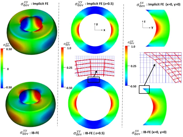
We also compare the deviatoric Cauchy stress components obtained from our IB-FE method with those obtained from the implicit FE method, when the radial displacement at the material point, (R = 0.5,Θ = 0, Z = 0.5) for both cases is the same. This is shown in Fig. 2. The distribution of σxydev,
predicted from the two methods looks almost identical. No leakage occurs even though the circumferential mesh size of the structure near the top is around six times of the fluid mesh size. We remark that a good performance of our IB-FE method is still achieved, even though the structure is largely deformed and the Lagrangian mesh size becomes much coarser than the Eulerian mesh.
1.0
-0.50 0.25
𝜎dev𝑦𝑦
: Implicit FE
: IB-FE : IB-FE ( z=0.5) 0
0.50
-0.50
𝜎dev𝑥𝑦
: IB-FE (x=0, y>0) 1.0
-0.50 0.25
𝜎dev𝑥𝑥
: Implicit FE (z=0.5)
𝜎dev𝑥𝑦
x y
y z
𝜎dev𝑥𝑦 𝜎dev𝑦𝑦
𝜎dev𝑦𝑦 𝜎dev𝑥𝑥
𝜎dev𝑥𝑥 : Implicit FE (x=0, y>0)
Fig. 2. Deviatoric Cauchy stress components from our IB finite element (IB-FE) method (bottom) versus those from implicit finite element (implicit FE) method (top).Left: the predicted xy-component Deviatoric Cauchy stress.Middle: the pre-dicted yy-component Deviatoric Cauchy stress in plane z=0.5. The fluid mesh (light blue) and deformed solid mesh (dark red) near the top is also shown. Right: the predicted xx-component Deviatoric Cauchy stress in the right half plane x=0. The fluid mesh (light blue) and deformed solid mesh (dark red) near the top is also shown.
3.2 Validation of the matrix material model: dilation of a long fiber-reinforced tube
val-idation study on dilation of a long fiber-reinforced cylindrical tube. The tube is also described in the cylindrical coordinates s = (R,Θ, Z). But the tube is much thinner and longer, and its initial stress-free configuration is 1.0 ≤
R ≤ 1.2,0 ≤ Θ ≤ 2π,0 ≤ Z ≤ 10. The tube is assumed to consist of an isotropic matrix and two families of continuous fibers running in the Θ, Z
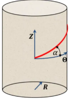
plane. We introduce the fiber angle to characterize the orientation of a family of fibers running in (Θ, Z) plane. The fiber angle is measured with respect to the circumferential orientation, ˆΘ, as shown in Fig. 3.
Fig. 3. Illustration of the fiber angle to characterize a fiber’s orientation. A tube is described in the cylindrical coordinatess= (R,Θ, Z). For a family of fibers running in (Θ, Z) plane, the fiber angel α is measured with respect to the circumferential orientation, ˆΘ.
Specifically, if the fiber angle isα, then the orientation of the fiber is (0 ˆR,cosαΘˆ,sinαZˆ). In this study, we take the fiber angles of the two families of fibers as α1 =α
and α2 = 180−α degree, respectively. And we specify the elastic model for
the matrix and fibers as below,
Ψ =Ψmatrix(I1) +Ψfb1(Ifb1) +Ψfb2(Ifb2), (61)
Ψmatrix(I1) =C1/2(I1−3), (62)
Ψfbi(Ifbi) =C2/2(
q
Ifbi−1)2,(i= 1,2). (63)
Similar to the first validation case, we fix the two ends of the tube through the penalty method. The fluid domain is −2.0≤x≤2.0,−2.0≤y≤2.0,−0.0≤
z ≤10.0. The density and viscosity of the fluid is set to be 1.0. We also specify a fluid sourceq(x, t) to dilate the tube,
q(x, t) =
q0(1.0−e−t) if (x2+y2 >0.42, z ∈[0.1,9.9]),
0 otherwise, (64)
whereq0 = 0.03125. The tube is discretized using eight-node hexahedral finite
elements, with the number of elements as (nR, nΘ, nZ) = (1,50,25). The fluid
is discretized based on the finite difference method, with the mesh-size as
hx =hy =hz = 0.1.
so-lution. Because fiber angles of the two fiber families sum up to 180 degree, the deformation of the tube can be shown to be axially symmetric (see Appendix B). Moreover, since the tube is very thin, the axial stretch is assumed to be uniform. Notice that this assumption is valid near the middle region of the tube. Based on those two conditions, we can derive an analytical expression for the inner pressure, Pinner (i.e. the pressure inside the tube), when the system
achieves the equilibrium.
Pinner =
Z Ro
Ri C1 r r2 R2 −
dr dR
!2
dr dRdR,
+ Z Ro
Ri
2C2 r
rcosα
R
2 1−1/
s
rcosα
R
2
+ (λzsinα)2
dr
dRdR. (65)
r and R are the deformed and initial radial coordinates, respectively. Ri and Roare the inner and outer radii, respectively. λz is the axial stretch ratio.α is
the fiber angle of one family of fibers, with the fiber angle of the other family as 180−α. If we know the deformed inner radius and outer radius, denoted as
ri and ro, we can obtain the current radial coordinate r(R) and axial stretch λz as below,
r(R) = v u u tR2
r2 o−r2i R2
o−Ri2
! +r2
i −R2i r2
o−r2i R2
o−Ri2
!
, (66)
λz =
R2o−R2i r2
o −r2i
. (67)
The details on the derivation of eqs. (65)-(67) are given in the Appendix B.
We simulate cases with different fiber angles α. For each fiber angle, we first obtain a transient case with the source term (64). We then restart simulations with zero source term at different restarting points to obtain several equilib-rium states. At each equilibequilib-rium state, we measure the ri, ro, and λz in the
middle of the tube, and the inner pressure, denoted as Pnumerical. We then
compute the analytical inner pressure, denoted asPanalytic based on measured
parameters and eqs. (65)-(67). We comparePnumerical and Panalytic, as listed in
Table 1. It can be seen, the errors in most cases are below 0.1 percent and in worst cases are below 4 percent.
4 Esophageal transport
La-Table 1
Error in the inner pressure for cases with different fiber angles, at different dilation levels.ri and ro is the deformed inner and outer radius in the middle section of the
tube, respectively. Pnumerical is the inner pressure in the middle section of the tube obtained from our simulations.Panalytic is the inner pressure based on eq. (65). The relative errorp =
|Pnumerical−Panalytic|
Panalytic
Fiber angle α (degree) ri ro Panalytic Pnumerical p
45 1.1345 1.313 0.0857 0.0830 3.15e-2
1.2636 1.428 0.1387 0.1388 7.21e-4
1.3850 1.537 0.1781 0.1777 2.25e-3
60 1.1332 1.312 0.0701 0.0676 3.57e-2
1.2632 1.427 0.1111 0.1105 5.40e-3
1.3875 1.539 0.1390 0.1388 1.44e-3
0 1.1312 1.310 0.1355 0.1343 8.86e-3
1.2524 1.417 0.2271 0.2264 3.08e-3
grangian mesh becomes much coarser than the fluid mesh. In this section, we proceed with our main application, which is a three-dimensional continuum-based model on esophageal transport.
4.1 Geometry, boundary conditions and material properties
The esophagus in the reference configuration is taken to be a long straight cylindrical tube. The geometry of the esophageal tube in this model is the same as our previous model [7], except that the esophagus’s length is taken to be 180 mm. We reduce the esophagus’s length from 240 mm to 180 mm in this model, because the esophageal tube modeled here does not include the lower and upper sphincters and thus is shorter than the entire esophagus. We model the esophageal wall as a three-layered composite, including the mucosa, CM and LM layers. We consider a thin liquid layer lining along the esophageal lumen when the esophagus is at rest, similar to previous models [7,28,29]. We calculate the thickness of each esophageal layer based on clinical data [14]. The lumen radius at rest is 0.3 mm. The thickness of mucosal, CM, and LM layers are 3.8 mm, 0.6 mm, and 0.6 mm, respectively.
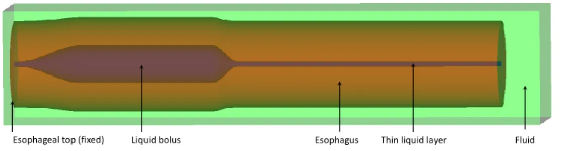
To use the IB-FE method, we immerse the entire esophagus in a fluid box of size (-7 mm, 7 mm) x (-7 mm, 7 mm) x (-126 mm, 180 mm). On the top surface of the fluid box, we specify zero-velocity boundary conditions to fix the esophageal top. This corresponds to the physiological constrains from the upper esophageal sphincter, which fixes the esophageal top in place. We also specify a penalty term to better fix the esophageal top. On the other surfaces of the fluid box, we impose traction-free boundary conditions. We simulate the transport of a bolus filled in the upper esophageal body initially. A schematic of the overall setup is shown in Fig. 4.
Liquid bolus Esophagus Thin liquid layer
Esophageal top (fixed) Fluid
Fig. 4. Schematic of the computational domain for the esophageal transport model. The elastic esophagus, a cylindrical tube is immersed in a background fluid box. The esophageal top is fixed. The upper esophagus is initially filled with a bolus and the lower part is filled with a thin liquid layer in the lumen. The top surface of the rectangular computational domain has zero-velocity boundary conditions. All the other five surfaces have traction-free boundary conditions.
elastic or pseudo-elastic material. However, quite different material models have been proposed among different groups [16,17,18,20,19]. Yang et al. [16] have proposed a so-called bi-linear model to characterize both the mucosal and muscle layers. Each esophageal layer is modeled as a fiber-reinforced material that consists of ground tissue (matrix) and elastic fibers. Natali et al. [18] also adopts a fiber-reinforced model to characterize mucosal and muscle layers, but the model is of an exponential form. Stavropoulou et al. [19] adopted Fung-type material models to characterize the mucosa and muscle layers, in which fiber model is not included. On the other hand, experiments on the histological information suggest both the mucosa and muscle layers are biological tissues embedded with biological fibers [18]. Therefore, we prefer to model esophageal layers as fiber-reinforced materials, especially when we need to include the active contraction/relaxation of muscle fibers. To test the capabilities of our model, we present three cases here. The first case is based on a bi-linear model proposed in [16]. The second case is based on an exponential model proposed in [18]. The third case is also based on a bi-linear model, but it includes more realistic and complicated muscle fiber architecture. The bi-linear model and the exponential model are discussed as below. Notice that the two models in their original forms include only two layers: mucosal and muscle layers. In our model, the muscle layers is split into two layers: CM and LM layers, to be consistent with more detailed histological information. For the material model on muscle fibers, we also introduce one additional parameter, referred here as the reference stretch ratio of fibers. This parameter is used to model neurally-controlled muscle activation, which will be discussed later.
4.1.1 Bi-linear model
This model is based on Yang et al. [16], in which they refer to the model as the bi-linear model. First is the mucosal layer. We remark that we adopt a different material model on mucosal layer. This is because the material model proposed in Yang et al. [16] is based on an vitro test. However, the in-vivo mucosal layer is substantially different from the in-vitro one in both the geometry and material behavior. The in-vivo mucosal layer is highly folded with a residual stress [30]. Its stiffness along the lateral direction is very low so that the esophageal tube attains a high distensibility, as seen in the clinical endoscopy, whereas the axial stiffness of mucosal layer is relatively high. Thus we model the mucosal layer here as a composite that is reinforced by a family fiber along the axial direction. The material model is as below,
Ψmucosa =Ψmatrixmucosa+Ψfibermucosa, (68)
Ψmatrixmucosa = C0
2 (I1−3), (69)
Ψfibermucosa = C1 2
" q
Imucosa
fb −1
2#
where Ifbmucosa = C : (amucosaN
amucosa). amucosa = (0 ˆR,0 ˆΘ,1 ˆZ), as the fiber angle of the axial fibers in the mucosal layer is 90 degree (i.e. along the axial direction).
Second is the CM layer. Its material model is as below,
ΨCM =ΨmatrixCM +ΨfiberCM, (71)
ΨmatrixCM = C2
2 (I1−3), (72)
ΨfiberCM = C3 2
q
ICM fb
λCM −1
2
, (73)
where IfbCM =C : (aCMN
aCM). aCM = (0 ˆR,cosαCMΘˆ,sinαCMZˆ). αCM is the fiber angle of the circular muscle fibers.λCMis the reference stretch ratio that
is included to deal with circular muscle fiber contraction.
Third is the LM layer. Its material model is as below,
ΨLM=ΨmatrixLM +ΨfiberLM, (74)
ΨmatrixLM = C5
2 (I1−3), (75)
ΨfiberLM = C6 2
q
ILM fb
λLM −1
2
, (76)
where IfbLM = C : (aLMN
aLM). aLM = (0 ˆR,cosαLMΘˆ,sinαLMZˆ). αLM is the fiber angle of the circular muscle fibers.
4.1.2 Exponential model
mucosal layer.
Ψmucosa =Ψmatrixmucosa+Ψfibermucosa, (77)
Ψmatrixmucosa = C0
2 (I1−3), (78)
Ψfibermucosa = C1 2
" q
Imucosa
fb1 −1
2#
+C2
k2 2 e k2 Imucosa fb2 (λmucosa
2 )2
−1
−k2(Ifb2mucosa−1)−1
+C3
k2 3 e k3 Imucosa fb3 (λmucosa
3 )2
−1
−k3(Ifb3mucosa−1)−1
, (79)
whereImucosa
fbi =C: (amucosai
N
amucosa
i ).amucosai = (0 ˆR,cosαimucosaΘˆ,sinαmucosai Zˆ). αmucosai is the fiber angle. In particular, α1mucosa = 90 degree, same as the bi-linear model.λmucosa
i is the reference stretch ratio under which the fiber elastic
potential is zero.
Second is the CM layer. The model includes ground tissue and one family of the circular muscle fibers as below,
ΨCM =ΨmatrixCM +ΨfiberCM, (80)
ΨmatrixCM = C4
k4
ek4(I1−3)−1, (81)
ΨfiberCM = C5
k2 5 e k5 ICM fb (λCM)2−1
−k5(IfbCM−1)−1
, (82)
where ICM
fb =C : (aCM
N
aCM). aCM = (0 ˆR,cosαCMΘˆ,sinαCMZˆ). αCM is the
fiber angle of the circular muscle fibers.λCMis the reference stretch ratio that is included to deal with circular muscle fiber contraction.
Third is the LM layer. The model includes ground tissue and one family of the longitudinal muscle fibers as below,
ΨLM =ΨmatrixLM +ΨfiberLM, (83)
ΨmatrixLM = C6
k6
ek6(I1−3)−1, (84)
ΨfiberLM = C7
k2 7 e k7 ILM fb (λLM)2−1
−k7(IfbLM−1)−1
, (85)
where ILM
fb = C : (aLM
N
aLM). aLM = (0 ˆR,cosαLMΘˆ,sinαLMZˆ). αLM is the
that is included to deal with longitudinal muscle fiber contraction.
4.2 Muscle activation
Neurally-controlled muscle activation provides the pumping force for bolus transport when the gravitational assistance is minimal. Two types of muscle activations, CM contraction and LM shortening, are involved as observed in studies based on in-vivo experiments [13,31]. CM contraction and LM short-ening occur as two synchronized traveling waves in the normal physiology. The two waves originate from the sequential contraction and relaxation of corre-sponding muscle fibers. However, the underlying process of neuronal firing or reaction kinematics at the continuum scale is still not available. Our previ-ous fiber-based method proposed a muscle-activation model by dynamically changing the rest lengths of springs that represent muscle fibers. Inspired by the success, here we apply the same idea to the continuum-based method. We model the muscle activation by dynamically changing the reference stretch ratio of corresponding muscle fibers. Specifically, letZ denote the vertical co-ordinate in the reference configuration of the esophageal tube. The bottom end of the esophagus is at the originZ = 0, and the top is atZ =L. The reference stretch ratio of a muscle fiber, denoted as (λmuscle(Z, t),muscle = CM or LM)
is given by
λmuscle(Z, t) =
1 if t−t0 ≤ L−cZ,
1−amuscle(Z, t) if L−cZ < t−t0 < L−cZ +∆cL,
1 if t−t0 ≥ L−cZ + ∆cL,
(86)
wherec is the speed of the activation wave,t0 is the initiation time of
activa-tion, and ∆Lis the contracting segment’s length in the reference configuration. Eq. (86) gives the reference stretch ratio of a fiber at its rest, activation, and relaxation states, respectively. The equation also shows that at any time, the whole esophageal tube has a contracting segment with a vertical length ∆L.
amuscle(Z, t) is referred to as the reduction ratio, whose form is the same as
our previous model [7],
amuscle(Z, t) =amuscle0 e−0.5(Z−Z0(t))2/W2, (87)
whereamuscle
0 is a constant reduction ratio,Z0(t) = c(t−t0) is theZ-coordinate
of the vertical center of the contraction segment, andW is the parameter that controls the width of the Gaussian distribution in eq. (87).
Table 2
Model parameters for the circular muscle (CM) contraction and longitudinal muscle (LM) shortening used in all the cases. The muscle activation model is based on eqs. (86) and (87) .
Muscle activation type a0 c(mm/s) ∆L (mm) W (mm) t0 (s)
CM contraction 0.4 100 60 15 0
LM shortening 0.4 100 60 15 0
4.3 Numerical issues
Esophageal transport model includes multiple length scales. This is evidenced by the fact that the esophageal length is 180 mm, while the lumen radius at rest is only 0.3 mm. The requirement of resolving the narrow lumen dic-tates the mesh size of the fluid grid. Moreover, very large deformation of a typical esophageal segment occurs when the bolus first comes in and then leaves. To deal with the leakage issue associated with large deformation of the Lagrangian mesh, our previous work employed a much refined mesh for inner-most esophageal layers. In this work, instead, we adopt the adaptive interaction quadrature rule that we discussed in Section 2. This approach per-mits us to use a relatively simple and coarse Lagrangian mesh for the solid. The Lagrangian mesh is based on the cylindrical coordinate system, with the mesh information of each layer listed in Table 3. The fluid mesh is a Cartesian mesh, with hx = hy = 0.2 mm and hz = 0.9 mm. The time step ∆t needs to
Table 3
Grid number along (R,Θ, Z) orientations, denoted as (nR, nΘ, nZ), for each layer
of the esophagus in the reference configuration.
Grid number Mucosal Layer CM LM
nR 6 1 1
nΘ 16 16 16
nZ 180 180 180
Table 4
Speed tests for cases with different interaction quadrature rules and the different number density based on the esophageal transport model. All cases run on the Northwestern super-computer, Quest, with 48 processors. Note that both the num-ber of the interaction quadrature points spread per time step and numnum-ber of time steps advanced per hour vary during the simulation. The reported values are ap-proximations to the average values.
Type of adap-tive interaction quadrature rule
number density
NO. of interaction quadrature points spread per time step (million)
NO. of time steps advanced per hour
Anisotropic rule 1.0 2.8 750
1.5 10 400
2.0 22 225
Isotropic rule 1.0 22 320
1.5 54 250
2.0 108 130
4.4 Results
4.4.1 Case 1: Esophageal transport using the bi-linear material model
devi-Table 5
Model parameters of the bi-linear model (i.e. Section 4.1.1).
Material type Material parameters
Mucosa C0(KPa) 4.0e-3 C1(KPa) 4.0e-2
CM C2(KPa) 4.0e-1 C3(KPa) 4.0
αCM(Deg.) 0
LM C5(KPa) 4.0e-1 C6(KPa) 4.0
αLM(Deg.) 90
disorder [31,35].
z
(m
m)
180
120
60
0
-7 0 x (mm) 7
(Pa)
t = 0s t = 0.6s t=1.2s t = 1.6s t = 2.4s 0
250 500
-500 -250
𝜎dev𝑦𝑦 𝑢𝑧 (cm/s)
0 10 20
-20 -10
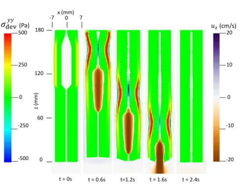
Fig. 5. Axial velocity of the bolus,uz, and the yy-compoent of the deviatoric stress
of the esophageal wall, σyydev, in the plane y = 0 at different times for Case 1 in Section 4.4.1.
4.4.2 Case 2: Esophageal transport using the exponential material model
Here we present our second case in which we use the exponential model (i.e. Section 4.1.2) for the material property of the esophagus. The material param-eters are listed in Table 6. Those paramparam-eters are based on Natali et al. [18]. We adjust the moduli of esophageal layers based on our previous studies and extensive empirical tests. This is because the original parameters from in-vitro tests yield much stiff esophageal muscle and mucosa. The muscle activation model is the same as Case 1, except that we adjust the modulus of muscle fibers when they are activated. This is because the stress is an exponential function of the stretch ratio in this case. Thus, the same amount of shortening as Case 1 will yield a very high active stress. In this case, we reduce C5 (or C7) to one fourth of the original value in Table 6, when a CM (or LM) fiber
z
(m
m
)
180
120
60
0
-7 0 x (mm) 7
(Pa)
t = 0s t = 0.6s t=1.2s t = 1.6s t = 2.4s 250
375 500
0 125
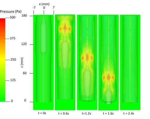
Pressure
Fig. 6. Pressure field in the plane y = 0 at different times for Case 1 in Section 4.4.1.
Table 6
Model parameters of the exponential model (i.e. Section 4.1.2 )
Material type Material parameters
Mucosa C0(KPa) 4.0e-2 C1(KPa) 4.0e-1
C2, C3(KPa) 4.98e-3 k2, k3 9.73e-2
αmucosa
2 (Deg.) 48.31 αmucosa3 (Deg.) 131.69
λmucosa2 , λmucosa3 5.0
CM C4(KPa) 2.17 k4 0.532
C5(KPa) 3.09 k5 0.532
αCM(Deg.) 0
LM C6(KPa) 2.17 k6 0.532
C7(KPa) 3.40 k7 0.899
αLM(Deg.) 90
infor-7
-7 0
y
(m
m)
-7 0 7
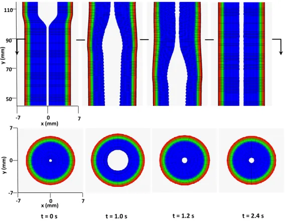
x (mm)
t = 0 s t = 0.8 s t = 1.2 s t = 2.4 s
50 70 90 110
-7 0 7
x (mm)
y
(m
m)
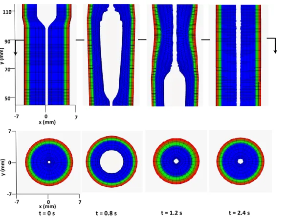
Fig. 7. Kinematics of the esophageal layers at four different stages: at rest (t = 0 s); at dilation (t = 0.8 s); at contraction (t = 1.2 s); and at relaxation (t = 2.4 s) for Case 1 in Section 4.4.1. The three layers included in the model, from the inside to the outside, are the mucosa, CM, and LM layers, respectively. (Upper) Side view of a section of the esophagus within the box: (-7 mm, 7 mm) x (-0.2 mm, 0.2 mm) x (45 mm, 115 mm); (Lower) top view of a section of the esophagus within the box: (-7 mm, 7 mm) x (-7 mm, 7 mm) x (89.5 mm, 90.5 mm).
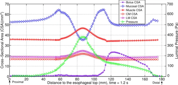
mation along the axial direction. The luminal pressure peak overlaps with the muscle CSA peak, indicating the synchrony between CM contraction and LM shortening. Compared with Case 1, the deformation of all esophageal layers in the contracted segment seems to be less significant. However, the peak pres-sure and the intra-bolus prespres-sure gradient is much higher. It seems that active contraction of an exponential fiber likely generates a higher squeezing effect.
4.4.3 Case 3: Esophageal transport including a more realistic and complex muscle fiber architecture
0 20 40 60 80 100 120 140 160 180 0
10 20 30 40 50 60 70
Distance to the esophageal top (mm), time = 1.2 s
Cross−Sectional Area (CSA)(mm
2 )
Luminal Pressure (Pa)
Bolus CSA Mucosal CSA Muscle CSA CM CSA LM CSA Pressure
600 700
500
400
300
200
100
0
Proximal Distal
Fig. 8. The cross-sectional area (CSA) of the bolus and the esophageal components, and the lumen pressure along its central line: x = 0, y = 0, at t = 1.2 s for Case 1 in Section 4.4.1.
z
(m
m)
180
120
60
0
-7 0 x (mm) 7
(Pa)
t = 0s t = 0.6s t=1.2s t = 1.6s t = 2.4s 0
600 1200
-1200 -600
𝜎dev𝑦𝑦 𝑢𝑧 (cm/s)
0 10 20
-20 -10
Fig. 9. Axial velocity of the bolus,uz, and the yy-compoent of the deviatoric stress
of the esophageal wall, σyydev, in the plane y = 0 at different times for Case 2 in Section 4.4.2.
ori-z
(m
m
)
180
120
60
0
-7 0 x (mm) 7
(Pa)
t = 0s t = 0.6s t=1.2s t = 1.6s t = 2.4s 250
375 500
0 125
Pressure
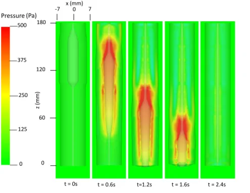
Fig. 10. Pressure field in the plane y = 0 at different times for Case 2 in Section 4.4.2.
entation varies spatially in a similar way. In particular, for the upper half esophageal body, we model the muscle fibers in both CM layer and LM layer as helical fibers. The fiber angels in CM layer and LM layer are 60 and 120 degree, respectively (i.e.αCM = 60, αLM= 120). For the lower half esophageal
body, we model the muscle fibers in CM layer and LM layer as circumferen-tial and axial fibers, respectively (i.e. αCM = 0, αLM = 90). An illustration is
shown in Fig. 13.
7
-7 0
y
(m
m)
-7 0 7
x (mm)
t = 0 s t = 1.0 s t = 1.2 s t = 2.4 s
50 70 90 110
-7 0 7
x (mm)
y
(m
m)
Fig. 11. Kinematics of the esophageal layers at four different stages: at rest (t = 0 s); at dilation (t = 1.0 s); at contraction (t = 1.2 s); and at relaxation (t = 2.4 s) for Case 2 in Section 4.4.2. The three layers included in the model, from the inside to the outside, are the mucosa, CM, and LM layers, respectively. (Upper) Side view of a section of the esophagus within the box: (-7 mm, 7 mm) x (-0.2 mm, 0.2 mm) x (45 mm, 115 mm); (Lower) top view of a section of the esophagus within the box: (-7 mm, 7 mm) x (-7 mm, 7 mm) x (89.5 mm, 90.5 mm).
0 20 40 60 80 100 120 140 160 180 0
10 20 30 40 50 60 70
Distance to the esophageal top (mm), time = 1.2 s
Cross−Sectional Area (CSA)(mm
2 )
Luminal Pressure (Pa)
Bolus CSA Mucosal CSA Muscle CSA CM CSA LM CSA Pressure
0 700
600
500
400
300
200
100
Proximal Distal
Fig. 12. The cross-sectional area (CSA) of the bolus and the esophageal components, and the lumen pressure along its central line: x = 0, y = 0, at t = 1.2 s for Case 2 in Section 4.4.2.
Helical CM fiber
(fiber angle = 60 degree)
Circumferential CM fiber
(fiber angle = 0 degree)
Middle position
(z=900 mm)
Helical LM fiber
(fiber angle = 120 degree)
Longitudinal LM fiber
(fiber angle = 90 degree)
Circular muscle (CM) Longitudinal muscle (LM)
Fig. 13. Illustration of the fiber architecture in the CM layer (left) and LM layer (right) in Case 3.
5 Conclusions
z
(m
m)
180
120
60
0
-7 0 x (mm) 7
(Pa)
t = 0s t = 0.6s t=1.2s t = 1.6s t = 2.4s 0
250 500
-500 -250
𝜎dev𝑦𝑦 𝑢𝑧 (cm/s)
0 10 20
-20 -10
Fig. 14. Axial velocity of the bolus, uz, and the yy-compoent of the deviatoric
stress of the esophageal wall,σyydev, in the plane y = 0 at different times for Case 3 in Section 4.4.3.
fiber-matrix interactions, and thus permits us to consider more realistic ma-terial behavior of biological tissues.
To validate our methodology, we first study a case in which a three-dimensional short tube is dilated. We compare results with those obtained based on the im-plicit FE method. Both the pressure-displacement relationship and the stress distribution matches very well. We remark that in our IB-FE case, the three-dimensional tube undergoes a very large deformation and the Lagrangian mesh becomes much coarser than the fluid mesh. To validate the performance of the method in handling fiber-matrix material models, we perform a second verifi-cation study on dilating a long fiber-reinforced tube. We study various cases with different fiber angles, and conduct comparisons between the computa-tional results and an analytic solution. The errors in most of the cases are less than one percent, with the largest error below 4 percent.
z
(m
m
)
180
120
60
0
-7 0 x (mm) 7
(Pa)
t = 0s t = 0.6s t=1.2s t = 1.6s t = 2.4s 250
375 500
0 125
Pressure
Fig. 15. Pressure field in the plane y = 0 at different times for Case 3 in Section 4.4.3.
model. The stress distribution shows clearly that the contractile stress comes from circular muscle contraction not the longitudinal muscle shortening. In-formation on the axial velocity, luminal pressure and kinematic inIn-formation is presented. They are consistent with the observation from our previous fiber-based model. We remark that one advantage of the continuum-fiber-based model over the traditional fiber-based model is its capability to handle more realistic and complicated material behavior. This is demonstrated in our third case, in which we include a spatially-varying muscle fiber architecture based on exper-iments. We find that this unique muscle fiber architecture could generate an interesting luminal pressure pattern that is observed clinically. The spatial-temporal luminal pressure profile has a pressure trough, clinically called as the pressure transition zone. This preliminary study suggests the muscle fiber architecture is likely to be responsible for the pressure transition zone. Future detailed investigation through case studies is recommended.
Acknowledgments
Experiment: Luminal pressure 0
75 150 Pressure (Pa)
Z(mm)
0 90 180
0 1.2 Time (s) 2.4
0 90 180
0 200 400 Pressure (Pa)
0 1.2 Time (s) 2.4
0 75 150 Pressure (Pa)
Z(mm)
0 90 180
0 1.2 Time (s) 2.4
Case 1: Luminal pressure Case 2: Luminal pressure
Case 3: Luminal pressure
Z Proximal
Distal Time
Pressure high
low
Fig. 16. Temporal-spatial profile of the luminal pressure (i.e. the pressure at
(x = 0, y = 0, z, t)) obtained from Case 1 (top left), Case 2 (top right), Case 3
(bottom left), and a clinical test on a normal people (bottom right).
Appendix A: IB-FE governing equations
The idea of the immersed boundary method is to separate the “fluid-like” components in the governing equations of the structure domain. Therefore, we derive another form of eq. (3) as below,
ρf ∂u s
∂t (x, t) +u
s(x, t)· ∇us(x, t)
!
− ∇ ·σ˜f,
=∇ ·∆σ−∆ρ ∂u s
∂t +u
s· ∇us
!
,
=fs, (88)
where σ˜f is the “fluid-like” stress that takes the same constitutive law as the fluid stress,σf. ∆σ =σs−σ˜f; ∆ρ=ρs−ρf.fs
is introduced to denote all the right-hand side of eq. (88).
At the fluid-structure interface, eq. (5) can also be written as
σf·n−σ˜f·n= ∆σ·n, (89)
the solid side.
We introduce a global velocity field, u(x, t), such that u(x, t)|Ωf(t) =uf(x, t), and u(x, t)|Ωs(t)=us(x, t).u(x, t) is continuous based on eq. (6). We consider the fluid as an incompressible Navier-Stokes fluid, then
σf=−pI+µ[∇u+ (∇u)T] in Ωf(t), (90)
σ˜f=−pI+µ[∇u+ (∇u)T] in Ωs(t), (91)
where pis the pressure to enforce the incompressibility condition.
Similarly, we introduce a global fluid source q(x, t), such that, q(x, t)|Ωf(t) =
qf(x, t), andq(x, t)|
Ωs(t) = 0. Since qf(x, t) is specified, we restrict it to vanish at the fluid-structure interface. Therefore,q(x, t) is continuous across the fluid-structure interface. Then we obtain new governing equations as below.
In the entire domain, Ω
ρf ∂u
∂t(x, t) +u(x, t)· ∇u(x, t)
!
=−∇p(x, t) +µ∇2u(x, t) +fs|
Ωs(t), (92)
∇ ·u(x, t) = q(x, t), (93)
where fs|Ωs(t) is only non-zero in the structure domain, Ωs(t).
At the fluid-structure interface, ∂Ωs(t)
[|σf|]·n=σf·n−σ˜f·n= ∆σ·n, (94)
[|u|] =uf−us = 0, (95) (96)
where [| · |] denotes a jump in a variable across the interface, i.e. the value on the fluid side minus the value on the structure side.
In the structure domain, Ωs(t)
fs =∇ ·∆σ−∆ρ ∂u s
∂t +u
s· ∇
us
!
. (97)
with the update Lagrangian description, as the structure is described in the current configuration.
In the entire domain, Ω
ρf ∂u
∂t(x, t) +u(x, t)· ∇u(x, t)
!
=∇ ·σf+ ¯fs
=∇p(x, t) +µ∇2u(x, t) + ¯fs, (98)
∇ ·u(x, t) =q(x, t), (99)
¯
fs = Z
Ωs(t)f
s
δ(x−χ(s, t))dχ(s, t)
−
Z
∂Ωs(t)∆σ·nδ(x−χ(s, t))da(χ(s, t)), (100)
where δ(x) is thed-dimensional delta function.
In the structure domain, Ωs(t)
fs =∇ ·∆σ−∆ρ ∂u s
∂t +u
s· ∇
us
!
. (101)
Notice that eqs. (92) and (94) are implied by eqs. (98) and (100). This can be shown as below.
For any x∈Ω\∂Ωs(t), the second term in eq. (100) drops, and eqs. (98) and (100) lead to eq. (92).
For any x ∈ ∂Ωs(t), we first pick a very small surface on the interface that
contains x, denoted as a. Then we pick a small control volume across a
with an infinitesimal width h, denoted as v. v has one face in the fluid
domain, denoted as af and one face in the structure domain, denoted as as.
An illustration in the two-dimensional case is shown in Fig. 17.
If we substitute eq. (100) into eq. (98) and integrate eq. (98) overv, we obtain
Z
v
ρf ∂u
∂t +u· ∇u
!!
dx−
Z
v
Z
Ωs(t)f
sδ(x−χ(s, t))dχ(s, t)
!
dx
= Z
v
∇ ·σfdx−
Z
v
Z
∂Ωs(t)∆σ·nδ(x−χ(s, t))da !
dx
=af(σf·n)−as(σ˜f·n)−a(∆σ·n). (102)