BAYESIAN IMAGE SEGMENTATION THROUGH LEVEL LINES SELECTION

BAYESIAN IMAGE SEGMENTATION THROUGH

LEVEL LINES SELECTION

C

HARLES

K

ERVRANN

INRA - Biom´etrie, Domaine de Vilvert, 78352 Jouy-en-Josas, France e-mail: [email protected]

(Accepted October 16, 2001)

ABSTRACT

Bayesian statistical theory is a convenient way of taking a priori information into consideration when inference is made from images. In Bayesian image segmentation, the a priori distribution should capture the knowledge about objects. Taking inspiration from (Alvarez et al., 1999), we design a prior density that penalizes the area of homogeneous parts in images. The segmentation problem is further formulated as the estimation of the set of curves that maximizes the posterior distribution. In this paper, we explore a posterior distribution model for which its maximal mode is given by a subset of level curves, that is the boundaries of image level sets. For the completeness of the paper, we present a stepwise greedy algorithm for computing partitions with connected components.

Keywords: area distribution, connected components, energy minimization, image segmentation, level curves.

INTRODUCTION

Image segmentation and object boundaries estimation are among the most challenging and fundamental addressed problems in image analysis (Mumford and Shah, 1989; Vincent and Soille, 1991; Morel and Solimini, 1994). Segmentation can be achieved by minimizing an energy model designed in conjunction with Bayes’s theorem as shown by Mumford and Shah (1989) and Zhu and Yuille (1996). Indeed, it is straightforward to transfer a Bayesian criterion into an energy minimization criterion (Morel and Solimini, 1994; Zhu and Yuille, 1996). Thereby, the discrete (Geman and Geman, 1984; Blake and Zisserman, 1987) or continuous (Mumford and Shah, 1989; Morel and Solimini, 1994) energy functional is traditionally comprised of two terms: the first term is a fidelity term describing the interaction between the observed data and the model (data model) and the second is a regularity term (prior model).

In Bayesian image segmentation, the prior model should capture the knowledge about objects. In particular, the incorporation of prior information about the outline of objects can be applied. There has been a growing interest in this field, particularly along the guidelines of Grenander’s general pattern theory using deformable templates (Grenander and Miller, 1994). In a separate way, Zhu and Yuille (1996) attempted to unify snakes (Kass et al., 1987) and region growing methods within a general energy/Bayes framework. Both approaches estimate the curves that maximally separate unknown statistics inside and outside the curves. Finally, the designed energy functionals are complex, for which it is

difficult to specify global minimizers corresponding to “best” segmentations. The maximum a posteriori (MAP) estimate is generally determined by prohibitive stochastic search procedures (Grenander and Miller, 1994) or other variants of steepest ascent algorithms (Zhu and Yuille, 1996). With these tools, additional a priori knowledge may be specified to ease the segmentation task: statistics inside region boundaries are assumed to be known (Grenander and Miller, 1994; Chan and Vese, 1999) or estimated using ad-hoc methods (Paragios and Deriche, 2000). In practical imaging, these methods still suffer from the problem of initialization of curves (Zhu and Yuille, 1996), off-line estimation of the mixture model of Gaussians approximating the probability density function of the image (Paragios and Deriche, 2000), or selection of hyperparameters weighting the contribution of energy terms (Zhu and Yuille, 1996; Chan and Vese, 1999; Paragios and Deriche, 2000).

THE BAYESIAN FRAMEWORK

Let S be an open subset (rectangle) of 2 and f a grey-scale image treated as a function defined on S. Below we will work in the continuous setup, where S is a subset of a Euclidian space and f : S

represents the observed data function. We use the terminology “site” or “pixel” to denote a point of the image, even in the continuous case. Each point x S is assigned

a grey value fx . According to Matheron (1975), we

interpret the image f as a family of sets defined by

Lτ f x S : fx τ , τ

. Each level set

Lτ f is assumed to be of finite perimeter. Therefore,

f will belong to the bounded variation (BV ) space as

shown by Alvarez et al. (1999).

Let Ω_i S

be a set of disjoint and non-empty

image domains or objects, and ∂Ω_i their boundaries.

A partition of the image domain S consists in finding a set Ω_i

P

i 1 and a background Ω defined as the

complementary subset of the union of objects Ω

S

P

i 1 Ωi, Ωi i

jΩj

/0 and Ω

i iΩ

/0. We

assume that the observed image f has been produced by the model f f

true ε, where ε is a

zero-mean Gaussian white noise: εx

iid

0σ

2

, x S.

The true image ftruex ∑ P

i 1fΩ

i1x Ω

i fΩ1

x Ω

is supposed piecewise constant, where f_Ω

iand fΩdenote

respectively the unknown average values of f overΩi

and Ω, and 1_x

E

is the set indicator function of the set E. The variance σ2 is assumed to be known and constant over the entire image. So, the likelihood for the data f given Ω₁ Ω

P is specified by

p fΩ

1 "!#!"!$ ΩP% ∝

exp&

1 2σ2

'

P

∑

i( 1) Ωi

fx

%

& f

Ωi%

2_dx

*

)

Ω fx

%

& f

Ω%

2_dx

+-, (1)

We seek a partition of the rectangle S into a finite set of objectsΩ_i, each of which corresponds to a part of the image where f is constant. Given the objects Ωi ,

the unknown background is explicitly determined as the complementary subset of the union of estimated objects. Therefore, we define the following collection

.

P of P 0 admissible, closed and connected

objects:

.

P / 0 Ω

1111 Ω

P

S ; S Ω

P

i 1

Ωi ; Ωi 1

2 i j2 P

Ωj /0 31 When P 0, there is no

object in the image. Following the Bayesian approach, we use some functional of the posterior distribution

pΩ

1Ω

P 4 f

∝ p f

4 Ω1

Ω

P πΩ

1Ω

P.

The likelihood p f

4 Ω1

5Ω

P is given by (1) and

πΩ

1Ω

P is the prior distribution of objects.

The posterior distribution is used in a further inferential issue concerning the objects within the Bayesian paradigm. The a priori distribution should

capture the knowledge about Ω₁5Ω

P . We

define a density that penalizes the area

4Ωi4

of objects. Additionally, the variables 4Ωi4

may be

considered as independent random variables with density g

4Ωi4

. Hence, the prior distribution is of the

form πΩ

1Ω

P6 Z7

1

p ∏

P

i 1

g

4Ωi4

a _{where Z}

p is

a normalization constant and a a real positive value. The density g

4Ωi4

is chosen to be a non-negative

monotically decreasing function of the object area

4Ωi4

. For instance, Alvarez et al. (1999) have empirically observed that the area distribution of homogeneous parts in images follows a power law β

4Ωi4

7

γ_{. In}

what follows, we shall consider this model for the density g

4Ωi4

. There are other possible choices of

g

4Ωi4

: the case of g

4Ωi4

∝exp89 β

4Ωi4

γ

related

to the Markov connected components fields, has been already discussed by Kervrann et al. (2000), Alvarez

et al. (1999) and Møller and Waagepetersen (1998).

BAYESIAN INFERENCE

All kinds of inference are made from

pΩ

1 Ω

P 4 f

. Finding the maximum a posteriori

(MAP) estimate is herein our choice of inference. As a consequence, the MAP estimation of objects is equivalent to the minimization of a global energy function E_λ fΩ

1111:Ω

P defined as

E_λ fΩ

1111Ω

P; E

pΩ

1111Ω

P

λEd

fΩ

1111: Ω

P< (2)

where

EpΩ

1111Ω

P6

P

∑

i 1

γlogΩ

i4

=8 A

is the penalty functional,

Ed fΩ

1111 Ω

P>

P

∑

i 1? Ωi

fx=8 fΩ

i

2

dx

? Ω

fx=8 f

Ω

2

dx

the data model, λ 2aσ

2 @

0 the regularization parameter and A logβ. The penalty functional

tends to regulate the emergence of objects Ω_i in the image. The regularization parameter λ can be then interpreted as a scale parameter that only tunes the number of regions (Morel and Solimini, 1994; Kervrann et al., 2000). If λ 0, each point is

potentially a region andΩ /0 ; the global minimum

coincides with zero and this segmentation is called the “trivial segmentation” (Morel and Solimini, 1994).

By using classical arguments on lower semi-continuous functionals on the BV space, we assume here the existence of minimizers of E_λ fΩ

1Ω

P

variation) (Morel and Solimini, 1994; Zhu and Yuille, 1996). Our MAP estimator is defined by (when it exists)

:AΩ

1111AΩB

P> argmin

02 P2 Targmin

C

Ω1DEEEDΩP

F

HG

P

E_λ fΩ

1111Ω

P< (3)

where .

P I

.

TKJ P L T , and T is the maximum

number of admissible objects registered in a bank

.

T.

We recall that ΩA

S M

B

P

i 1

A

Ωi is the complementary

subset of estimated objects NAΩ

11115AΩB

P . A direct

minimization with respect to all unknown domains

Ω_i and parameters f_Ω

i is a very intricate problem,

even if T is low since objects are not designated. In what follows (Lemma 1), we prove that the object boundaries that minimize E_λ fΩ

1111:Ω

P are level

lines of the function f , which makes the problem tractable.

LEMMA 1 If there exist minimizers and no pathological minimum exists, then the energy minimizing set of curves is a subset of level lines of

f , i.e. the border∂ΩA

i of eachΩA

i is a boundary of a

connected component of a level set of f .

Proof of Lemma 1. Let Ω_δ be a variation of a set Ω, i.e. the Hausdorff distance d∞Ω

δΩL δ . To

prove Lemma 1, we assume that, for any connected perturbation of Ω such that d∞Ω

δΩOL δ, two

neighboring sets Ω and ΩP do not merge into one

single setΩ ΩP and, for any connected perturbation

of Ω such d∞Ω

δΩQL δ, Ω does not split into two

new sets. This corresponds to prohibited topological changes. Without loss of generality, we prove Lemma 1 for one object Ω and a background Ω, that is the closure of the complementary set ofΩ. For two sets A and B such that B

I

A, we denoteR

ASB

f defTR

Af 8UR

Bf .

Then, we have

∆ΩV

) Ωδ

W

Ω1

def

VXΩ

δ$&YΩ and

Z

)

Ω_δf[

2

&]\

)

Ωf^

2 V 2 ) Ωf ) Ω_δ W Ωf * Z ) Ω_δ W

Ωf[

2

, (4)

We define∆E_λ fΩ_ E

λ fΩ

δ`8 E

λ fΩ9 T

1

T₂ T3 T4 T5, where

T₁ V

) Ωδ

f2&

) Ω

f2

T₂ V

1 Ω ) Ω_δ W Ωλγ

T₃ V &

1

Ω

δ

Z

)

Ω_δ f

[ 2 * 1 Ω \ ) Ωf ^ 2

T₄ V

)

S

W

Ω_δ f

2 & ) S W Ωf 2

T₅ V &

1

S$&OΩ

δ

Z

)

S

W

Ω_δ f

[

2

* 1

S$&YΩ

\ ) S W Ωf ^ 2 , (5)

By definition we have T₁ T4

0. Passing to the

limit∆

4Ω4

0, we obtain expressions for T

2T

3and T5 (higher order terms are neglected)

T₂ V

λγ

Ω

) Ωδ

W

Ω1

T₃ V &

2 Ω ) Ω_δ W Ωf )

Ωf &

1 Ω Z ) Ω_δ W

Ωf[

2

* 1

Ω

2

) Ωδ

W Ω1 \ ) Ω f^ 2

T₅ V

1

S$&OΩ

'

2

) Ωδ

W

Ωf)

S

W

Ωf

&

Z

) Ωδ

W Ωf [ 2 & 1

S$&YΩ

) Ω_δ W Ω1 \ ) S W Ω f ^ 2

+ , (6)

We define the image moments m₀ R

Ω1, m1

R Ωf , K

0 aR

S1, K1 bR

Sf . Using the mean value

theorem for a double integral, which states that if f is continuous and a connected subset E is bounded by a simple curve, then for some point x₀ in E we have

R

E fxdE fx

0c

4E4 where 4E4 denotes the area of

E, it follows that

∆E_λ f Ω

%

V d

M₀

e fg h

i

m2₁ m2 0

&

K

1& m

1%

2

K

0& m

0% 2 * λγ m₀ j * M₁

e fg h

i

2K

1& m

1%

K₀& m

0

&

2m₁ m₀

j

fx

0%

&

K₀ m₀K

0& m

0%

fx

0%

2

)

Ω_δ

W

Ω1k

)

Ω_δ

W

Ω1,

(7)

Let x_b be a fixed point of the border ∂Ω. Choose Ω_δ such that ∂Ω_δ ∂Ω except on a small

neighborhood of x_b. The energy having a minimum for

Ω, fx

b needs to be solution of the following equation

∆E_λ fΩ

∆4Ω4

mlM

0 M1f

x

b#n

O

By passing to the limit∆4Ω4

0, we obtain M

0

M₁fx

bo 0. This equation has a unique solution.

The coefficients M₀ and M₁ depend on neither x_bnor

fx

b, and M

0 p

0. The function f is continuous and ∂Ωis a connected curve. Therefore fx

b is constant

when x_bcovers∂Ω. This completes the proof.

A STEPWISE GREEDY ALGORITHM FOR IMAGE SEGMENTATION

To implement our level set image segmentation based on energy minimization, a four step method is used. The proposed algorithm is not a region growing algorithm (Morel and Solimini, 1994) since all objects are built once and for all. It differs from the watershed approach since regions that emerge from the watershed segmentation are not necessarily connected components within the image level sets (Vincent and Soille, 1991). Let K,λ, 4Ωmin4 be the input parameters

set by the user.

Bilevel set construction. The first step completes a quantization of the function f ql f

min fmaxn in

K r 4:8 non-equal-sized and non-overlapping

intervals lt l

7

1t

l , l X 1: K . Given this set of

intervals estimated using the maximum entropy sum method (Kapur et al., 1985), let b_l be the bilevel set image with b_lx< 1 if fxslt

l

7

1t

l and b

lx< 0

otherwise. The connected components of bilevel sets can be characterized by their surrounding curves, that is the level lines. If we map these level lines for a given set of K levels, we get a segmentation of the image also called topographic map (Caselles et al., 1999). More generally, one can consider a segmentation achieved using only some connected components of bilevel sets, which is the philosophy of our approach. The most perceptible level lines could be determined by the detection of T-junctions of level lines (Caselles et al., 1999). Instead, we use herein a simpler criterion where perceptually significant level lines are the bilevel sets boundaries of an quantized image by using K quantizers and an entropy method. The entropy method due to Kapur et al. (1985) chooses the thresholds t_l

to be the values at which the information is maximum.

Object extraction. A crude way to build pixels sets corresponding to objects is to proceed to a connected components labeling of bilevel set images

b_l and to associate each label with an object Ω

i.

Though this process may work in the noise-free case, in general we would also need some smoothing effect of the connected components labeling. So, we consider a size-oriented morphological operator acting on sets that consists in keeping all connected components of the output of area larger than a limit 4Ωmin4. This connected operator in mathematical

morphology will never introduce new features or edges and boundaries of remain connected components are preserved (Salembier and Serra, 1995). The list of connected components then forms the bank

.

T of

admissible objects Ω₁111 Ω

T with

4Ωi4

4Ωmin4

.

Configuration determination. The connected components are then combined during the third step to form object configurations. For instance, these configurations can be built by enumeration of all possible object combinations, i.e. 2T configurations. Each configuration is made of a subset of connected components taken in the bank .

T. The background Ω corresponds to the complementary set of objects selected for each configuration.

Energy computation and object configuration selection. Energy calculations take the image intensities of the original (not quantized) image to establish piecewise-constant approximation errors. Energies of the form R

Ωi

fxQ8 fΩ

i

2 _dx

are

computed once and stored on a RAM memory. The energy term R

Ω fx8 f

Ω

2 _{dx is efficiently} updated for each configuration. For a fixed bank

.

T t Ω

1: Ω

T , one way to choose the optimal

set of of objects ΩA

1: ΩA B

P ,

A

P L T , is to search for

all possible combinations of P objects and compute the corresponding energy E_λ fΩ

15Ω

P. Enumerating

all possible sets of objects in the object bank and comparing their energies is computationally too expensive if T is large. Instead of a such brute force search, we propose a stepwise greedy algorithm for minimizing E_λ fΩ

15Ω

P . We start from P 0

and introduce one object Ω_j at a time. At the first step, we compute the T energies with one single object Ωj at once against the complementary subset

Ω Su

T

j i 1Ωi

. Let ΩA

1 be the estimated object that best lowers E_λ fΩ

1: Ω

P . This object is

stored on a RAM memory as an object of the optimal configuration. It is removed from the initial bank

.

T.

At any step of the algorithm, a new object is chosen to maximally decrease the energy E_λ fΩ

1Ω

P .

Suppose that at the P-th step,P andA

A

Ωare not known but we have estimated P objects NAΩ

1AΩ

P and

a current background Ω S - ΩA

1: ΩA

P . Let

E_λ fAΩ

15AΩ

P be the current computed energy.

Then at the P

1

-th step, we choose the object

Ωj

.

T v NAΩ

1AΩ

P which has the maximal

difference, i.e.

A

Ω_P

1 arg max

ΩjwG

TS

C

B

Ω1DxxxD

B

ΩPFzy

E_λ fAΩ

1AΩ

P

8 E

λ fAΩ

1AΩ

PΩ

The algorithm stops at the P-th step when the addition of any object does not decrease E_λ fΩ

1: Ω

P .

This means that the optimal number of objects is PA

P and the remaining objects of the bank

are a part of the estimated background ΩA

S

A

Ω15ΩA B

P . This algorithm selects a suboptimal

configuration of objects corresponding to a local minimum. Using this algorithm, at most T }~T

1: 2 object configurations are examined.

EXPERIMENTAL RESULTS

Experiments were conducted on satellite and medical images. The number of bilevel sets K was set fairly low (K 4 or K 8) to obtain large regions

and to improve robustness to noise and artifacts in the image. Regions with areas4Ωi4€

l01000101001n‚}

4S4

are discarded. To estimate A andγ, we consider the sets of observations log

4Ωi4

ƒlogg

4Ωi4

ƒ1 L i L

T . We perform a linear regression on this set so as

to find the straight line (in the log-log coordinates) logg

4Ωi4

:„ A8 γlog

4Ωi4

closest to the data in

the least squares sense (Alvarez et al., 1999). The choice of the hyperparameter λ determines mostly

the properties of the segmentation result. If f is a function from S to l0255n, a default choice for the

hyperparameter isλ ~l01111n=} 255

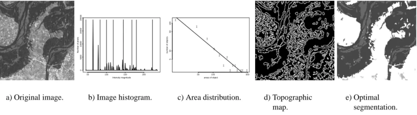
2_{. Fig. 1a shows} an aerial 256 } 256 image (in the visual spectrum)

depicting the region of Saint-Louis during the rising of the Mississippi and Missouri rivers in July 1993. We are interested in extracting the rivers and a background corresponding to textured urban areas. Fig. 1 shows the segmentation results when K 8,

4Ωmin4

0100025}

4

S

4

and λ 0125 } 255

2_{. In this experiment, the} maximum number of significant components is T

291. The corresponding topographic map is shown in Fig. 1d. The image histogram has been quantized with K 8 quantizers and an entropic method (Fig.

1b). We estimated the values of parameters A 31727

and γ 11486 by linear regression (Fig. 1c). In that

case, the residual sum of squares is 21007 and 17 L

4Ωi4

L 21886 10

4 _{pixels. It takes about 15 seconds} (25 095 €

T }…T

1

: 2 42 486 iterations) of

computing time for building

.

T and selecting the

best configuration shown in Fig. 1e (P 105 objects)

using the stepwise greedy algorithm (λ 0125 }

2552). Enumerating all the configurations is infeasible since 2T

3198 10

87 _{iterations! The non-connected} background is labeled in “white” in Fig. 1e and the objects are filled with their mean gray values f_Ω

i

.

a) Original image.

Intensity magnitude

Number of pixels

50 100 150 200

0

5000

10000

15000

20000

b) Image histogram. •

•

• •

• •

•

• • •

•• • • areas of object

number of objects

50 100 500

5

10

50

100

c) Area distribution. d) Topographic map.

e) Optimal segmentation.

Fig. 1. Segmentation of a (256 } 256) satellite image (K 8,

4Ωmin4

0100025}

4

S

4

,λ 0125} 255

2_).

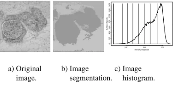
Finally, the performance of the segmentation procedure is demonstrated for a (181 } 217) MR

image shown in Fig. 2 and a microscopic medical breast (256 } 256) image shown in Fig. 3. In Fig. 2,

the dark background has been previously eliminated before processing. Segmentation of both grey and white matter is achieved using the set of parameters

K 8,λ 015} 255

2_and

4Ωmin4

010001}

4S4. Fig.

3 exhibits an inflammatory carcinoma with metastases. Fig. 3b shows the segmentation results when K 8,

4Ωmin4

01001}

4S4 andλ

015} 255

2_.

a) MR image.

b) Image segmen-tation.

c) Boun-daries.

Intensity magnitude

Number of pixels

0 50 100 150 200†

250

†

0

500

‡

1000

1500

d) Image histogram.

a) Original image.

b) Image segmentation.

Intensity magnitude

Number of pixels

100 150 200ˆ

0

200

‰

400

Š

600

800

‹

1000

1200

1400

c) Image histogram.

Fig. 3. Segmentation of a microscopic image.

CONCLUSION AND

PERSPECTIVES

In this paper, we have presented a Bayesian approach for extracting structures in images. Although our work is related to morphological approaches based on connected operators (Salembier and Serra, 1995), it is an independent approach since we seek minimizers of a global objective functional. In addition, we proved that our MAP estimator can be determined by selecting a subset of image level lines. A total CPU time of a few seconds on a 296 MHz workstation makes the method attractive for many time-critical applications. In terms of future directions for research, we propose to create a non-linear scale-space by successive applications of an area morphology operator to select most meaningful regions in the image.

REFERENCES

Alvarez L, Gousseau Y, Morel JM (1999). Scales in natural images and a consequence on their bounded variation. In: Nielsen M, Johansen P, Olsen OF, Weickert J, eds. Scale-Space Theories in Computer Vision. Berlin, Heidelberg: Springer, 247-58.

Blake A, Zisserman A (1987). Visual Reconstruction. Cambridge, Mass.: MIT Press.

Caselles V, Coll B, Morel JM (1999). Topographic maps and local contrast changes in natural images. Int J Comput Vision 33(1):5-27.

Chan T, Vese L (1999). Active contour model without edges. In: Nielsen M, Johansen P, Olsen OF, Weickert J, eds. Scale-Space Theories in Computer Vision. Berlin, Heidelberg: Springer, 141-51.

Geman S, Geman D (1984). Stochastic relaxation, gibbs distributions, and the bayesian restoration of images. IEEE T Pattern Anal 6(6):721-41.

Grenander U, Miller MI (1994). Representations of knowledge in complex systems. J Roy Stat Soc B Met 56(4):549-603.

Kapur JN, Sahoo PK, Wong AKC (1985). A new method for gray-level picture thresholding using the entropy of the histogram. Comput Vision Graph 29:273-85.

Kass M, Witkin A, Terzopoulos D (1987). Snakes: active contour models. Int J Comput Vision 12(1):321-31. Kervrann C, Hoebeke M, Trubuil A (2000). Level lines

as global minimizers of energy functionals in image segmentation. In: Vernon D, ed. Computer Vision – ECCV 2000, 6th European Conference on Computer Vision, Dublin, Ireland, July 26 – July 1, 2000, Proceedings, Part II. Berlin, Heidelberg: Springer, 241-56.

Matheron G (1975). Random Sets and Integral Geometry. New York: John Wiley.

Møller J, Waagepertersen RP (1998). Markov connected component fields. Adv Appl Probab 30: 1-35.

Morel JM, Solimini S (1994). Variational methods in image segmentation. Boston: Birkhauser.

Mumford D, Shah J (1989). Optimal approximations by piecewise smooth functions and variational problems. Commun Pur Appl Math 42(5):577-685.

Paragios N, Deriche R (2000). Coupled geodesic active regions for image segmentation: a level set approach. In: Vernon D, ed. Computer Vision – ECCV 2000, 6th European Conference on Computer Vision, Dublin, Ireland, July 26 – July 1, 2000, Proceedings, Part II. Berlin, Heidelberg: Springer, 224-40.

Salembier P, Serra J (1995). Flat zones filtering, connected operators, and filters by reconstruction. IEEE T Image Process 4(8):1153-60.

Vincent L, Soille P (1991). Watershed in digital spaces: an efficient algorithm based on immersion simulations. IEEE T Pattern Anal 13(6):583-98.