SUPERVISED AUTOMATIC HISTOGRAM CLUSTERING AND
WATERSHED SEGMENTATION. APPLICATION TO MICROSCOPIC
MEDICAL COLOR IMAGES
O
LIVIERL
EZORAYLUSAC EA 2607, IUT Saint-Lô, 120 rue de l'Exode, 50000 Saint-Lô, FRANCE e-mail: [email protected]
(Accepted June 12, 2003)
ABSTRACT
In this paper, an approach to the segmentation of microscopic color images is addressed, and applied to medical images. The approach combines a clustering method and a region growing method. Each color plane is segmented independently relying on a watershed based clustering of the plane histogram. The marginal segmentation maps intersect in a label concordance map. The latter map is simplified based on the assumption that the color planes are correlated. This produces a simplified label concordance map containing labeled and unlabeled pixels. The formers are used as an image of seeds for a color watershed. This fast and robust segmentation scheme is applied to several types of medical images.
Keywords: clustering, color, histogram, segmentation, watershed.
INTRODUCTION
Color image segmentation refers to the partitioning of a multi-channel image into meaningful objects. The various approaches to color image segmentation reported in the literature may be roughly classified into a few categories: clustering methods (Park etal., 1998), edge-based methods (Carron and Lambert, 1994), region growing methods (Trémeau and Borel, 1998), and variational methods (Kichenassamy et al., 1995). In the context of segmenting medical color images, we propose to combine two types of methods: clustering- and region growing- methods. Both methods are based on the watershed principle (Soille, 1999). Because clustering methods relying on the 3D information of a color histogram may be time-consuming (Géraud et al., 2001), methods based on the multi-thresholding of the color planes may be preferred (Soille, 2000; Albiol et al., 2001). Herein, we intend to use the merging of segmentation maps obtained by treating the color planes independently (marginal approach to color segmentation) as the
GRAY-SCALE IMAGE PLANES
CLUSTERING
Each color plane is here clustered independently by splitting its (gray-scale) histogram in several sections corresponding to representative classes of pixels in the image. We assume that the number Nc of classes of pixels is a priori known. Furthermore, we suppose that the representative sections (or clusters) of each color plane histogram are located around its main modes. It is thus reduced to find the threshold values dissecting the histograms in a finite number of clusters. This is here achieved by computing the 1D watershed of the complement (Hc) of each color plane histogram (H) as reported in Soille (1999).
Using all the minima of Hc as seeds for the 1D watershed would result in a severe over-clustering. In this respect, only the so-called h-minima constrain the watershed growing. In the process of extracting the h-minima, h is experimentally defined as:
( )
H
-
max
( )
H
σ
=
h
, (1)scale image is defined by the label value of the section p belongs to in the clustered histogram.
The essential drawback of the method is the number of resulting sections, generally larger than the desired number of classes Nc. Adjacent sections of the histogram are accordingly merged according to the following strategy. A 1D adjacency graph of the clustered histogram is first built, and the section showing the smallest number of pixels in the histogram is identified. The current smallest section is then merged with that one of its two adjacent sections (Si) minimizing the following quantity:
( ) ( ) ( ) ) i S ( l ) i S ( u k H i i S u S l
k
‡”
=, (2)
Where a histogram section is denoted by Si, H(k) is the number of pixels of gray-level k, and l(Si) (resp.
u(Si)) is the lowest (resp. highest) gray level in section Si. The adjacency graph is updated each time
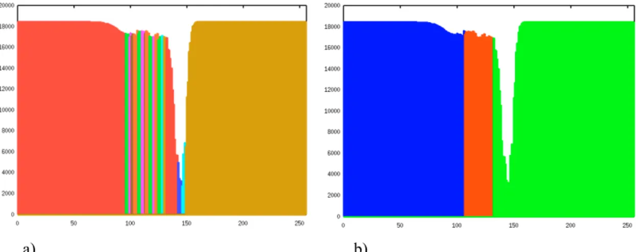
two sections merge and the algorithm iterates till the number of sections in the histogram is equal to Nc. Fig. 1 illustrates various steps of the clustering in 3 sections of a color plane histogram (the original color image associated to Fig. 1 is displayed in Fig. 5a). We can note in Fig. 1 that the three final sections correspond to the main three peaks of the histogram
and that the zone of influence of each peak is well defined. Of course, the merging step is not performed when the number of the sections resulting from the watershed is lower than Nc.
MERGING OF THE SEGMENTED
COLOR PLANES
Concordance of the marginal labels
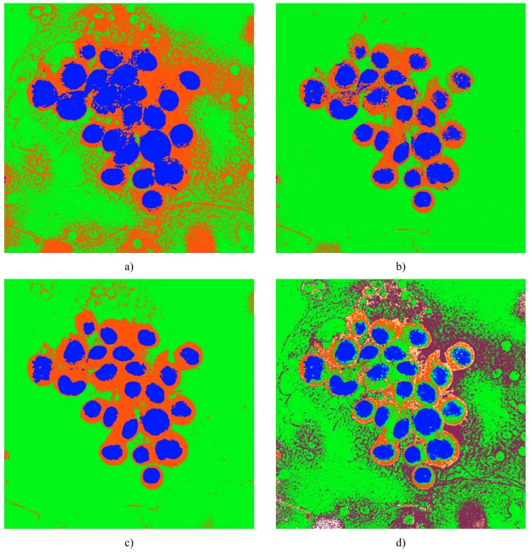
In color images, the three color planes express a priori different types of information. In this respect, the spatial regions exhibited with a marginal segmentation (every color plane clustered independently) may differ depending on the color plane which is considered. This is illustrated by Figs. 2a-c showing for each color plane (R, G, B) the segmentation map obtained through the clustering approach of the previous section with Nc=3. The main objective of color segmentation is to take advantage of the information available with several color channels. Along that line, one approach to color image segmentation consists in blending the information carried by the segmentation maps of the different channels (Figs. 2a-c). The resulting map is often referred to as the so-called label concordance map (Richards and Jia, 1999; Kurugollu et al., 2001). The label concordance map (Fig. 2d), denoted by J, is here derived as the intersection of the three marginal segmentation maps.
a) b)
a)
c)
b)
d)
SIMPLIFICATION OF THE
CONCORDANCE MAP
Due to the intersection, the number of clusters in the image J may be higher than the desired number of clusters Nc. Herein, we propose to use a simplification operator in order to reduce the number of clusters associated to the concordance map. We assume that the representative clusters of a color image shall be those associated to the largest areas in the concordance map. In other words, the representative clusters shall be defined as the combinations of marginal labels showing the largest overlaps across the marginal segmentation maps. It is here the right point to emphasize that the more the three marginal segmentation maps overlap, the more the color planes are correlated (and the smaller is the number of labels in the concordance map). Fig. 2d illustrates this point on an experimental basis. The simplification of the label concordance map (Fig. 2d) consists accordingly in keeping only the most representative combinations of labels. Altogether, such simplification is based on the idea that the color planes are correlated. In fact this is often the case for microscopic images. In particular, an experimental study carried on many hematological and serous microscopic images revealed that the correlation rate between the three color planes is commonly higher than 90% in the RGB color space.
To perform the simplification, the histogram of the concordance map J is first computed. Each peak in the histogram corresponds to the number of pixels of a class in image J. The simplification operator may be defined as follows. Let M be the set of all the local maxima in the histogram Hj of J:
M= {supq Hj(x) | q ∈ V(x)} (4)
Where sup is the supremum and V(x) is the neighborhood of a current concordance label (denoted by x) (here, the two adjacent concordance labels in the histogram). M(Nc) is the set of concordance labels associated to the Nc greatest maxima of the histogram in the set M. The simplification may so be expressed as: if, for a pixel p of J, J(p) ∉ M(Nc) then J(p)=0 else J(p) remains unchanged. The resulting simplified image includes
Nc+1 classes. The labeled pixels are associated to the
Nc most representative clusters of the concordance image. Pixels labeled as 0 (referred to as unlabeled hereafter) are considered as uncertain pixels since
Fig. 3. The label concordance map after simplification: black pixels correspond to unlabeled pixels. The labeled pixels correspond to the three different classes of pixels (background, cytoplasm and nucleus) and will be used as markers for the color watershed.
COLOR WATERSHED
Instead of using classical probability values (Bloch, 1996) to assess the basic assignment of unlabeled pixels (black pixels in Fig. 3) to a cluster, we propose to use a color watershed. The seeds for the watershed are provided by the labeled connected components of the simplified concordance image If. This is necessary to let the regions grow independently one of the other.
Aggregation function
The color watershed used in this paper is defined according to a specific aggregation function. The aggregation (or distance) function estimates the certainty that a pixel p belongs to an adjacent region
f(p,Ri)=(1 - α) ||I
( )
Ri - I(p) || + α || ∇I(p) ||. (5) This function combines local information (the modulus of the color gradient), and global information in the form of a (statistical) comparison between the color of a pixel p and the mean color of its neighbor region Ri (performed with the Euclidean distance). During the growing process, every time a pixel is added to a region Ri, the mean color of the region is updated. Both the color image and the gradient image are normalized before the watershed growing in order to have the same range of values. In Eq. (5), the blending coefficient α allows to tune the influence of the local and global criteria during the growing process. The watershed uses the value of the aggregation function f as the ordering of a classical FIFO priority queue (Vincent and Soille, 1991). Pixels are assigned to the region corresponding to the smallest value of f as reported in Salembier et al.(1996).
Estimation of alpha
The α parameter was introduced to control the relative influence of the global and local criteria. α may be fixed once for all according to some a priori knowledge on the images (Lezoray et al., 2000). However, an adaptable segmentation modifying the value of α across the iterations seems more suitable. The initial value of α is 0, and α is so allowed to evolve during the growing. At each iteration k, the quantity Vk=∑ f(p,Ri) is computed where Vk relates to the set of unlabeled pixels p currently processed (the set of processed pixels is a subset of all the unlabeled pixels and concerns only unlabeled pixels currently adjacent to a given region). Therefore, V0 gives an initial value relating to the unlabeled pixels of the image adjacent to the markers at the first iteration. Since the initial value of α is 0, V0 quantifies the initial global similarity between unlabeled pixels and region markers. If the global similarity Vk is small, the unlabeled pixels are close to the regions so that α shall be small to essentially take into account the global information. On the contrary, if Vk increases, α shall increase to give more weight to the local information. To fulfill these requirements α is defined by:
Table 1 gives the mean value of α during the growing for 10 different medical images (cytology, hematology, skin, brain, histology, etc.) One shall note the quite different mean values of α listed in table 1. The proposed automatic evolution of α obviously avoids the difficulty to tune this parameter according to some a priori knowledge (which is very difficult to express numerically). Fig. 4 illustrates the variations of α across the iterations of the watershed region growing process applied to Fig. 3. The visual evaluation of the segmented images confirms that the self-adaptable segmentation gives the more accurate results.
Table 1. Mean value of α for several medical images.
Image α Nc
I1 0.054 2
I2 0.037 2
I3 0.212 2
I4 0.191 2
I5 0.207 2
I6 0.078 3
I7 0.051 3
I8 0.216 4
I9 0.188 4
I10 0.216 4
Fig. 4. An example of variation of the alpha parameter (obtained on the watershed growing of Fig. 3).
RESULTS
information provided by the color watershed algorithm allows to complete the segmentation.
a)
b)
Fig. 5. (a) The original microscopic image: cells from serous cytology stained by the Papanicolaou protocol (b) Final regions obtained after the watershed growing initialized on the labeled regions of the simplified concordance map (Fig. 3).
The influence of the choice of the color space onto the current color image segmentation method, has been studied. Indeed, the correlation between the color planes is an important property in our approach to color segmentation. Because the strength of the correlation may vary with the color space, its choice may influence the output of the method. To address the later point, we used a database of 63 hematological color images available on the internet network for e-learning and e-diagnosis purposes. The point of the segmentation exercise is here to extract the cells in the images, and moreover to provide a classification of the cells into Nc=3 classes.
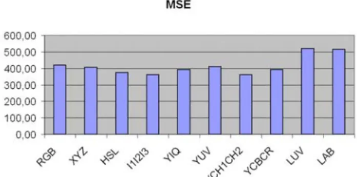
To compare the different color spaces for the image database (mention RGB, XYZ, HSL, I1I2I3,
YIQ, YUV, Ych1Ch2, YcbCr, L*u*v*, L*a*b*), a Mean Squared Error (MSE) is computed between the original image and a colorized image where each pixel carries the mean color value of the connected component it belongs after the segmentation; the lower the MSE, the better the segmentation. Fig. 6 shows that some color spaces seem more adapted than others. In this respect, the color space relevance shall be studied and quantified with an appropriate measure for each considered application.
Fig. 6. The MSE obtained for several color spaces.
a)
b)
c)
CONCLUSION
A supervised method for segmenting microscopic color images has been discussed and illustrated. In a first step, for each color plane, distinct segmentation maps are extracted by a marginal approach. Their intersection, the so-called label concordance map, is then simplified. The simplification relies on the assumption that the color planes are correlated and leaves some pixels unlabeled. A self-adaptable region growing method is last performed to obtain the final regions. The proposed method is reliable and fast and provides a classification of each region among a predefined number of classes. Further research concerns the automatic determination of the number of classes to be used in the segmentation for indexing color medical images.
REFERENCES
Adams R, Bischof L (1994). Seeded region growing. IEEE Transactions on Pattern Analysis and Machine Intelligence (PAMI) 16(6):641-7.
Albiol A, Torres L, Delp Ed (2001). An unsupervised color image segmentation algorithm for face detection applications. In: Proceedings. of the IEEE International Conference on Image Processing, 3.
Bloch I (1996). Information combination operators for data fusion. IEEE transactions on Systems, Man and Cybernetics 26(1):52.
Carron T, Lambert P (1994). Color edge detector using jointly hue, saturation and intensity. In: Proceedings of the IEEE International Conference on Image Processing (ICIP) 3:977.
DiZenzo S (1986). A note on the gradient of a multi-image. Computer Vision, Graphics and Image Processing (CVGIP) 33:116.
Géraud T, Strub P-Y, Darbon J Color (2001) Image Segmentation Based on Automatic Morphological Clustering. In: Proceedings. of the IEEE International Conference on Image Processing 3:70-73.
Kichenassamy S, Kumar A, Olver PJ, Tannenbaum A, Yezzi A (1995). Gradient flows and geometric active contours. In: Proceeding of the International Conference on Computer Vision (ICCV), 810.
Richards J, Jia X (1999). Remote sensing digital image analysis. Spinger-Verlag.
Salembier P, Brigger P, Casas J.R, Pardàs M (1996). Morphological operators for image and video compression, IEEE transactions on image processing 5(6):881-97
Serra J. (1982). Image Analysis and mathematical morphology. London: Academic Press.
Soille P (1999). Morphological Image Analysis, Principles and applications, Springer-Verlag.
Soille P (2000). Morphological image analysis applied to crop field mapping. Image Vis Comp 18(13):1025-32. Trémeau A, Borel N (1998). A region growing and
merging algorithm to color segmentation. Patt Recog 30(7):1191.