Scalability Evaluation of Cimmino Algorithm
for Solving Linear Inequality Systems
on Multiprocessors with Distributed Memory
∗ Irina M. Sokolinskaya1, Leonid B. Sokolinsky1c
The Authors 2018. This paper is published with open access at SuperFri.org
The paper is devoted to a scalability study of Cimmino algorithm for linear inequality systems. This algorithm belongs to the class of iterative projection algorithms. For the analytical analysis of the scalability, the BSF (Bulk Synchronous Farm) parallel computation model is used. An implementation of the Cimmino algorithm in the form of operations on lists using higher-order functionsMap andReduce is presented. An analytical estimation of the scalability boundary of the algorithm for cluster computing systems is derived. An information about the implementation of Cimmino algorithm on lists in C++ language using the BSF program skeleton and MPI parallel programming library is given. The results of large-scale computational experiments performed on a cluster computing system are demonstrated. A conclusion about the adequacy of the analytical estimations by comparing them with the results of computational experiments is made.
Keywords: system of linear inequalities, iterative algorithm, projection algorithm, Cimmino algorithm, parallel computation model, bulk synchronous farm, scalability estimation, speedup, parallel efficiency, cluster computing systems.
Introduction
The problem of solving systems of linear inequalities arise in numerous fields. As examples, we can mention linear programming [1, 2], image reconstruction from projections [3], image pro-cessing in magnetic resonance imaging [4], intensity-modulated radiation therapy (IMRT) [5]. At the present time, a lot of methods for solving systems of linear inequalities are known, among which we can mark out a class of self-correcting iteration methods that allow efficient paralleliza-tion. In this field, pioneer works are papers [6, 7], in which the Agmon–Motzkin–Schoenberg re-laxation method for solving systems of linear inequalities was proposed. The rere-laxation method belongs to the class of projection methods, which use the operation of orthogonal projection onto a hyperplane in Euclidean space. One of the first iterative algorithms of projection type was the Cimmino algorithm [8], intended for solving systems of linear equations and inequalities. Cimmino algorithm had a great influence on the development of computational mathematics [9]. A considerable number of papers have been devoted to the generalizations and extensions of the Cimmino algorithm (for example, see [3, 10–13]).
In many cases, systems of linear inequalities arising in the solution of practical problems can involve up to tens of millions of inequalities and up to hundreds of millions of variables [2]. In this case, the issue of developing scalable parallel algorithms for solving large-scale systems of linear inequalities on multiprocessor systems with distributed memory becomes very urgent. When one creates parallel algorithms for large multiprocessor systems, it is important at an early stage of the algorithm design (before coding) to obtain an analytical estimation of its scalability. For this purpose, one can use various models of parallel computation [14]. Nowadays, a large number of different parallel computation models are known. The most famous models among them are PRAM [15], BSP [16] and LogP [17]. Each of these models generated a large
∗The article is recommended for publication by the Program Committee of the International Scientific Conference
“Russian Supercomputing Days 2018”.
family of parallel computation models, which extend and generalize the parent model (see, e.g., [18–20]). The problem of developing new parallel computation models is still important today. The reason is that it is impossible to create a parallel computation model, which is good in all respects. To create a good parallel computation model, the designer must restrict the set of target multiprocessor architectures and class of algorithms. In paper [21], the parallel computation model BSF (Bulk Synchronous Farm) intended for cluster computing systems and iterative algorithms was proposed. The BSF model makes it possible to predict the scalability boundary of an iterative algorithm with great accuracy before coding. An example of using the BSF model is given in [22].
The purpose of this article is to investigate the scalability of the Cimmino algorithm for solv-ing large-scale systems of linear inequalities on multiprocessor systems with distributed memory by using the BSF parallel computation model. The rest of the article is organized as follows. Section 1 gives a formal description of the Cimmino algorithm. In Section 2, the representation of the Cimmino algorithm in the form of operations on lists using higher-order functions Map
and Reduce defined in the Bird–Meertens formalism is constructed. Section 3 is dedicated to an analytical investigation of the scalability of the Cimmino algorithm on lists using the BSF model cost metrics; the equations for estimating the speedup and parallel efficiency are given; the boundary of the algorithm scalability depending on the problem size is calculated. In Sec-tion 4, a descripSec-tion of the implementaSec-tion of the Cimmino algorithm on lists in C++ language using the BSF algorithmic skeleton and the MPI parallel programming library is presented; a comparison of the results obtained analytically and experimentally is given. In conclusion, the obtained results are summarized and directions for further research are outlined.
1. Cimmino Algorithm for Inequalities
Let us consider the system of linear inequalities
li(x) =hai, xi −bi60 (i= 1, . . . , m), (1)
where hai, xi is the Euclidean inner product of ai and x in Rn, bi ∈ R. To avoid triviality, we
assumem>2. We also assume that the system (1) is consistent. It is necessary to find a solution of the system of linear inequalities (1). To solve this problem, it is convenient to use a geometric language. Thus, we look uponx= (x1, . . . , xn) as a point inn-dimensional Euclidean spaceRn,
and each inequality li(x)60 as a half-space Pi. Therefore, the set of solutions of system (1) is
the convex polytope M = Tm
i=1
Pi. Each equation li(x) = 0 defines a hyperplane Hi:
Hi ={x∈Rn| hai, xi=bi}. (2)
Let the orthogonal projection of x ∈ Rn onto the hyperplane H
i ⊂ Rn be denoted by πHi(x).
The orthogonal projection πHi(x) can be calculated by the following equation:
πHi(x) =x+
bi− hai, xi
kaik2
ai, (3)
where k·k is the Euclidean norm. Let us define the orthogonal reflection of x with respect to hyperplaneHi as follows:
ρHi(x) =πHi(x)−x=
bi− hai, xi
kaik2
The Cimmino algorithm for equally weighted inequalities consists of the following steps:
Step 1: k:= 0;x0 :=0.
Step 2: xk+1:=xk+mλ m
P
i=1
ρHi(xk).
Step 3: If kxk+1−xkk2 < ε then go to Step 5.
Step 4: k:=k+ 1; go to Step 2.
Step 5: Stop.
Cimmino’s method starts with an arbitrary point x0 in Rn as an initial approximation,
and then calculates at each step the centroid of a system of masses placed at the reflections of the previous iterate with respect to the hyperplanes H1, . . . , Hm defined by the system of
inequalities. This centroid is taken as the new iterate:
xk+1=xk+
λ m
m
X
i=1
ρHi(xk). (5)
In equation (5), λ is a relaxation parameter. It is known [10] that for 0 < λ <2 the iteration process (5) converges to a point belonging to the polytopeM.
2. Cimmino Algorithm in the Form of Operations on Lists
In order to obtain analytical estimations of an algorithm using the cost metrics of the BSF model, it must be represented in the form of operations on lists using higher-order functions
Map and Reduce defined in the Bird–Meertens formalism [23]. The higher-order function M ap
applies the given function F :A→ B to each element of the given list [a1, . . . , am] and returns
a list of results in the same order:
M ap(F,[a1, . . . , am]) = [F(a1), . . . , F(am)]. (6)
The higher-order function Reduce reduces the given list [b1, . . . , bm] to a single value by
itera-tively applying the given binary associative operation ⊕:B×B→ Bto each pair of elements:
Reduce(⊕,[b1, . . . , bm]) =b1⊕. . .⊕bm. (7)
In the context of the Cimmino algorithm, we define the list Lmap as follows:
Lmap = [i1, . . . , im], (8)
where ik∈ {1, . . . , m} and ik 6=il fork6=l (k, l = 1, . . . , m). In other words, Lmap – is the list
of numbers of inequalities (1) ordered in an arbitrary way. For an arbitrary pointx∈Rn, let us
define the function Fx :{1, . . . , m} →Rnas follows:
Fx(i) =ρHi(x) (9)
for all i ∈ {1, . . . , m}. In other words, the function Fx(i) calculates the orthogonal reflection
of x with respect to the hyperplane Hi. For an arbitrary point x ∈ Rn, let us define the list
L(reducex) ⊂Rn as follows:
The list L(reducex) holds orthogonal reflections of the point x with respect to the hyperplanes
H1, . . . , Hm in the order determined by the listLmap. Thus, the listL(reducex) is obtained from the
listLmap by applying to it the higher-order functionM apusing as a parameter the functionFx:
L(reducex) =M ap(Fx, Lmap). (11)
Let us define the binary associative operation⊕:Rn×Rn→Rn as follows:
x⊕y=x+y (12)
for all x, y ∈ Rn. In this case, the ⊕ operator performs the conventional composition of vec-tors. Then the sum of orthogonal reflections of the point x can be obtained by applying to the list L(reducex) the higher-order function Reduce using as a parameter the vector composition operation ⊕:
m
X
i=1
ρHi(x) =Reduce(⊕, L (x)
reduce). (13)
Now we can write theCimmino algorithm in the form of operations on lists:
Step 1: k:= 0;x0 :=0;Lmap := [1, . . . , m].
Step 2: L(xk)
reduce:=M ap(Fxk, Lmap).
Step 3: s:=Reduce(⊕, L(xk)
reduce).
Step 4: xk+1:=xk+mλs.
Step 5: If kxk+1−xkk2 < εthen go to Step 7.
Step 6: k:=k+ 1; go to Step 2.
Step 7: Stop.
The BSF model assumes that the algorithm is executed by a computing system consisting of one master-node andK worker-nodes (K >0). Step 1 of the algorithm is performed by both the master and the workers during the initialization of the iterative process. Step 2 (Map) is performed only on the worker-nodes. Step 3 (Reduce) is performed on the worker-nodes and partially on the master-node. Steps 4–6 are performed only on the master-node. The BSF model assumes that all arithmetic operations (addition and multiplication) as well as comparison op-erations on floating-point numbers take the same time τop.
3. Analytical Evaluation of Scalability
Let us introduce the following notation for the scalability evaluation of the Cimmino algo-rithm:
cs : the quantity of float numbers transferred from the master to one
worker;
cmap : the quantity of arithmetic operations performed in theMap step
(Step 2 of the algorithm);
ca : the quantity of arithmetic operations required to calculate the sum of two
cr : the quantity of float numbers transferred from one worker to the
master;
cp : the quantity of arithmetic and comparison operations performed by the master in
Steps 4 and 5 of the algorithm.
Let us calculate the indicated values. At the beginning of each iteration, the master sends to all the workers the current approximation xk, which is a vector of dimensionn. Hence:
cs=n. (14)
Let us calculate the number of arithmetic operations performed in the Map step. For each el-ement of the list Lmap, one vector is calculated by equation (4). Note that the values ofkaik2
(i= 1, . . . , m) do not depend onxk, and therefore can be calculated in advance at the
initializa-tion stage. Taking this into account, the quantity of operainitializa-tions for calculating one orthogonal reflection of the point xk is 3n+ 1. Multiplying this value by the number of inequalities, we
obtain
cmap=m(3n+ 1). (15)
During the execution ofReduce step, the listLreduceconsisting ofmvectors is divided into equal
parts, each of them assigned to a single worker. Everywhere below we assume that K6m. For simplicity we assume that m is a multiple of number of workers K. The composition of vectors of dimensionn requiresnarithmetic operations. Hence:
ca=n. (16)
After execution of Reduce step, each worker sends the resulting vector to the master. Thus:
cr =n. (17)
The execution of Step 4 requires 2n operations (we assume the constant value of λ/m to be computed in advance). The execution of Step 5 requires 3n−1 arithmetic operations and one comparison operation. It follows the equation:
cp = 5n. (18)
Let us designate the time spent by the worker to perform one arithmetic operation as τop,
and designate the time spent for transferring a single float number across the network excluding latency as τtr. In that way, we get the following values for the cost parameters of the BSF
model [21] in the case of the Cimmino algorithm:
ts=nτtr; (19)
tmap=m(3n+ 1)τop; (20)
ta=nτop; (21)
tr=nτtr; (22)
Equation (19), obtained on the basis of (14), gives an estimation of the time ts spent by the
master to transfer a message to one worker excluding latency. Equation (20) is obtained using the equation (15). According to the BSF model cost metric,tmap denotes the total time spent by a
single worker to process the entireMap list. Equation (21) obtained using equation (16) calculates the time tp spent by a processor node on adding two vectors of dimension n. Equation (22),
obtained on the basis of (17), gives an estimation of the time tr spent by the master to transfer
a message to one worker excluding latency. Equation (23) obtained using equation (18) calculates the time tp spent by the master on the following actions: calculating the next approximation
and checking of the stopping criterion. In accordance with this metric, the time for solving the problem by a system consisting of one master and one worker (K = 1) can be estimated as follows:
T1= 2L+ts+tr+tp+tM ap+lta
= 2(L+τtrn) +τop(5n+m(3n+ 1) + (m−1)n).
(24)
The time of solving the problem by a system composed of one master and K workers can be estimated by the following equation:
TK=K(2L+ts+tr+ta) +
tM ap+lta
K −ta+tp
= 2K(L+τtrn+τopn) +τop
m(3n+ 1) + (m−1)n
K + 4n
.
(25)
For m→ ∞, the equations (24) and (25) asymptotically tend to the following estimations:
T1 = 2(L+τtrn) +τop(5n+m(3n+ 1) +mn) ; (26)
TK = 2K(L+τtrn+τopn) +τop
m(3n+ 1) +mn
K + 4n
. (27)
On the basis of equations (26) and (27) we can write the equation for speedup ain the form of a function of K:
a(K) = T1
TK
= 2(L+τtrn) +τop(5n+m(3n+ 1) +mn) 2K(L+τtrn+τopn) +τop
m(3n+1)+mn K + 4n
. (28)
To determine the scalability boundary of the Cimmino algorithm in accordance with the procedure described in [21], let us deduce the derivative a0(K) and solve the equation
a0(K) = 0. (29)
Using simple algebraic transformations, from equation (28), we can deduce the following equation for the derivative of speedup:
a0(K) = (2(L+τtrn) +τop(5n+m(3n+ 1) +mn))·
·
m(3n+1)+mn
K2 τop−2(L+nτtr)−τopn
2K(L+τtrn+τopn) +τop
m(3n+1)+mn K + 4n
2.
Let us solve the equation
(2(L+τtrn) +τop(5n+m(3n+ 1) +mn))·
·
m(3n+1)+mn
K2 τop−2(L+nτtr)−τopn
2K(L+τtrn+τopn) +τop
m(3n+1)+mn K + 4n
2 = 0.
(31)
Dividing both sides of equation (31) by the positive quantity
2(L+τtrn) +τop(5n+m(3n+ 1) +mn)
and multiplying by the positive quantity
2K(L+τtrn+τopn) +τop
m(3n+ 1) +mn
K + 4n
2
we obtain the equation
m(3n+ 1) +mn
K2 τop−2(L+nτtr)−τopn= 0,
which implies
K =
s
(m(3n+ 1) +mn)τop
2(L+nτtr) +nτop
.
Thus, equation (31) has the only root
K0 =
q
(m(3n+ 1) +mn)τop/(2(L+nτtr) +nτop)
on the interval [1,+∞). It is easy to see that the derivative a0(K) calculated by the equa-tion (30) takes only positive values in the interval [1, K0) and only negative values in the interval
(K0,+∞). Therefore, the pointK0is the maximum of the functiona(K) on the interval [1,+∞).
It follows that the maximum of speedup is obtained at the point K0. Thus, in accordance with
the BSF model, the boundary Kmax of the scalability of the Cimmino algorithm is determined
by the following equation:
Kmax=
s
(m(3n+ 1) +mn)τop
2(L+nτtr) +nτop
. (32)
Let us simplify equation (32). For n, m→ ∞, we have
(m(3n+ 1) +mn)τop≈O(mn) (33)
and
2(L+nτtr) +nτop≈O(n). (34)
Substituting the right-hand sides of equations (33) and (34) into (32), we obtain
Kmax =
s
O(mn)
O(n) ,
which is equivalent to
Kmax=
p
In that way, the boundary of the scalability of the Cimmino algorithm on lists increases in proportion to the square root of the numberm of inequalities. In conclusion of this section, let us write the equation for estimating the parallel efficiency e as a function of K. Considering equation (28), we have
e(K) = a(K)
K =
2(L+τtrn) +τop(5n+m(3n+ 1) +mn)
2K2(L+τ
trn+τopn) +τop(m(3n+ 1) +mn+ 4nK)
. (36)
4. Numerical Experiments
In order to verify the analytical results, we implemented the Cimmino algorithm in C++ language using the BSF algorithmic skeleton and the MPI parallel programming li-brary. The source code of this program is freely available on Github, at https://github.
com/leonid-sokolinsky/BSF-Cimmino. The system of inequalities was taken from the model
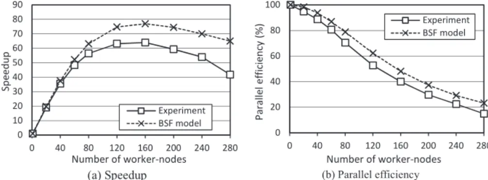
scalable linear-programming problem Model-n given in [24]. In this system, the number of in-equalities is m = 2n+ 2, where n is the dimension of the space. We investigated the speedup and parallel efficiency of the Cimmino algorithm on the supercomputer “Tornado SUSU” [25]. The calculations were performed for the dimensions 1 500, 5 000, 10 000 and 16 000. At the same time, we plotted the curves of speedup and parallel efficiency for these dimensions using equa-tions (28) and (36). For this, the following values in seconds were determined experimentally:
L = 1.5·10−5, τop = 2.9·10−8 and τtr = 1.9·10−7. The results are presented in Fig. 1–4.
In all cases, the analytical estimations were very close to experimental ones. Moreover, the performed experiments show that the boundary of the BSF-program scalability increases in pro-portion to the square root of the number m of inequalities. It was analytically predicted by the equation (35).
Conclusion
In this paper, the scalability and parallel efficiency of the iterative Cimmino algorithm used to solve large-scale linear inequality systems on multiprocessor systems with distributed memory were investigated. To do this, we used the BSF (Bulk Synchronous Farm) parallel computation model based on the “master-slave” paradigm. The BSF-implementation of the Cimmino algo-rithm in the form of operations on lists using higher-order functionsMapandReduceis described. A scalability boundary of the BSF-implementation of the Cimmino algorithm is obtained. This estimation tells us the following. If space dimension nis greater than or equal to the numberm
of inequalities, then the boundary of the scalability of the Cimmino algorithm on lists increases in proportion to the square root of the number m of inequalities. So, we may conclude that the Cimmino algorithm on lists is scalable well. Also, the equations for estimating the speedup and parallel efficiency of the Cimmino algorithm on lists are obtained. The implementation of the Cimmino algorithm in C++ language using the BSF algorithmic skeleton and the MPI parallel programming library was performed. This implementation is freely available on Github,
at https://github.com/leonid-sokolinsky/BSF-Cimmino. On a cluster computing system,
(a) Speedup (b) Parallel efficiency 0 5 10 15 20 25 30
0 40 80 120 160 200 240 280
S p e e d u p
Number of worker-nodes Experiment BSF model 0 20 40 60 80 100
0 40 80 120 160 200 240 280
P a ra ll e l e ff ic ie n cy ( % )
Number of worker-nodes Experiment BSF model
Figure 1.Experiments for n= 1 500 andm= 3 002
(a) Speedup (b) Parallel efficiency
0 5 10 15 20 25 30 35 40 45
0 40 80 120 160 200 240 280
S p e e d u p
Number of worker-nodes Experiment BSF model 0 20 40 60 80 100
0 40 80 120 160 200 240 280
P a ra ll e l e ff ic ie n cy ( % )
Number of worker-nodes Experiment BSF model
Figure 2.Experiments for n= 5 000 andm= 10 002
(a) Speedup (b) Parallel efficiency
0 10 20 30 40 50 60 70
0 40 80 120 160 200 240 280
S p e e d u p
Number of worker-nodes Experiment BSF model 0 20 40 60 80 100
0 40 80 120 160 200 240 280
P a ra ll e l e ff ic ie n cy ( % )
Number of worker-nodes Experiment BSF model
Figure 3. Experiments for n= 10 000 andm= 20 002
(a) Speedup (b) Parallel efficiency
0 10 20 30 40 50 60 70 80 90
0 40 80 120 160 200 240 280
S p e e d u p
Number of worker-nodes
Experiment BSF model 0 20 40 60 80 100
0 40 80 120 160 200 240 280
P a ra ll e l e ff ic ie n cy ( % )
Number of worker-nodes
Experiment BSF model
1) apply the Cimmino algorithm to implement the Qwest phase of the NSLP algorithm [2], designed to solve large-scale non-stationary linear programming problems;
2) carry out computational experiments to solve large-scale linear programming problems on a cluster computer system under the conditions of dynamically changing the input data.
Acknowledgments
The study was partially supported by the RFBR according to research project No. 17-07-00352-a, by the Government of the Russian Federation according to Act 211 (con-tract No. 02.A03.21.0011) and by the Ministry of Science and Higher Education of the Russian Federation (government order 2.7905.2017/8.9).
This paper is distributed under the terms of the Creative Commons Attribution-Non Com-mercial 3.0 License which permits non-comCom-mercial use, reproduction and distribution of the work without further permission provided the original work is properly cited.
References
1. Cottle, R.W., Pang, J.-S., Stone, R.E.: The Linear Complementarity Problem. Society for Industrial and Applied Mathematics (2009)
2. Sokolinskaya, I., Sokolinsky, L.B.: On the Solution of Linear Programming Problems in the Age of Big Data. In: Parallel Computational Technologies, PCT 2017. Communica-tions in Computer and Information Science, vol. 753, pp. 86–100. Springer, Cham (2017), DOI: 10.1007/978-3-319-67035-5 7
3. Censor, Y., Elfving, T., Herman, G.T., Nikazad, T.: On Diagonally Relaxed Orthog-onal Projection Methods. SIAM Journal on Scientific Computing 30, 473–504 (2008), DOI: 10.1137/050639399
4. Zhu, J., Li, X.: The Block Diagonally-Relaxed Orthogonal Projection Algorithm for Com-pressed Sensing Based Tomography. In: 2011 Symposium on Photonics and Optoelectronics, SOPO. pp. 1–4. IEEE (2011), DOI: 10.1109/SOPO.2011.5780660
5. Censor, Y.: Mathematical optimization for the inverse problem of intensity-modulated radi-ation therapy. In: Palta, J.R., Mackie, T.R. (eds.) Intensity-Modulated Radiradi-ation Therapy: The State of the Art. pp. 25–49. Medical Physics Publishing, Madison, WI (2003)
6. Agmon, S.: The relaxation method for linear inequalities. The Canadian Journal of Mathe-matics 6, 382–392 (1954), DOI: 10.4153/CJM-1954-037-2
7. Motzkin, T.S., Schoenberg, I.J.: The relaxation method for linear inequalities. The Canadian Journal of Mathematics 6, 393–404 (1954), DOI: 10.4153/CJM-1954-038-x
8. Cimmino, G.: Calcolo approssimato per le soluzioni dei sistemi di equazioni lineari. La Ric. Sci. XVI, Ser. II, Anno IX, 1. 326–333 (1938)
Bologna (Ciclo di Conferenze in Ricordo di Gianfranco Cimmino, 2004). pp. 87–109. Tecno-print, Bologna, Italy (2005)
10. Censor, Y., Zenios, S.A.: Parallel Optimization: Theory, Algorithms, and Applications. Oxford University Press, New York (1997)
11. Censor, Y., Elfving, T.: New methods for linear inequalities. Linear Algebra Appl. 42, 199– 211 (1982), DOI: 10.1016/0024-3795(82)90149-5
12. Censor, Y.: Sequential and parallel projection algorithms for feasibility and optimization. In: Censor, Y., Ding, M. (eds.) Proc. SPIE 4553, 25 Sept. 2001. Visualization and Op-timization Techniques, pp. 1–9. International Society for Optics and Photonics (2001), DOI: 10.1117/12.441550
13. Kelley, C.T.: Iterative Methods for Linear and Nonlinear Equations. Society for Industrial and Applied Mathematics, Philadelphia (1995)
14. Bilardi, G., Pietracaprina, A.: Models of Computation, Theoretical. In: Encyclopedia of Parallel Computing. pp. 1150–1158. Springer US, Boston, MA (2011), DOI: 10.1007/978-0-387-09766-4
15. JaJa, J.F.: PRAM (Parallel Random Access Machines). In: Encyclopedia of Parallel Com-puting. pp. 1608–1615. Springer US, Boston, MA (2011), DOI: 10.1007/978-0-387-09766-4 23
16. Valiant, L.G.: A bridging model for parallel computation. Communications of the ACM 33, 103–111 (1990), DOI: 10.1145/79173.79181
17. Culler, D., Karp, R., Patterson, D., Sahay, A., Schauser, K.E., Santos, E., Subramo-nian, R., von Eicken, T.: LogP: towards a realistic model of parallel computation. In: Proceedings of the fourth ACM SIGPLAN symposium on Principles and practice of par-allel programming, PPOPP’93. pp. 1–12. ACM Press, New York, New York, USA (1993), DOI: 10.1145/155332.155333
18. Forsell, M., Leppanen, V.: An extended PRAM-NUMA model of computation for TCF programming. In: Proceedings of the 2012 IEEE 26th International Parallel and Distributed Processing Symposium Workshops, IPDPSW 2012. pp. 786–793. IEEE Computer Society, Washington, DC, USA (2012), DOI: 10.1109/IPDPSW.2012.97
19. Gerbessiotis, A.V.: Extending the BSP model for multi-core and out-of-core computing: MBSP. Parallel Computing 41, 90–102 (2015), DOI: 10.1016/j.parco.2014.12.002
20. Lu, F., Song, J., Pang, Y.: HLognGP: A parallel computation model for GPU clus-ters. Concurrency and Computation Practice and Experience 27, 4880–4896 (2015), DOI: 10.1002/cpe.3475
22. Sokolinskaya, I., Sokolinsky, L.B.: Scalability Evaluation of NSLP Algorithm for Solving Non-Stationary Linear Programming Problems on Cluster Computing Systems. In: Su-percomputing, RuSCDays 2017. Communications in Computer and Information Science, vol. 793, pp. 40–53. Springer, Cham (2017). DOI: 10.1007/978-3-319-71255-0 4
23. Cole, M.I.: Parallel programming with list homomorphisms. Parallel Processing Letters 05, 191–203 (1995), DOI: 10.1142/S0129626495000175
24. Sokolinskaya, I., Sokolinsky, L.: Revised Pursuit Algorithm for Solving Non-stationary Lin-ear Programming Problems on Modern Computing Clusters with Manycore Accelerators. In: Supercomputing, RuSCDays 2016. Communications in Computer and Information Science, vol. 687, pp. 212–223. Springer, Cham (2016), DOI: 10.1007/978-3-319-55669-7 17